Abstract
In recent times, there has been a notable global phenomenon characterized by a double predicament arising from the concomitant rise in worldwide life expectancy and a significant decrease in birth rates. The emergence of this phenomenon has posed a significant challenge for governments worldwide. It not only poses a threat to the continued viability of state-funded welfare programs, such as social security, but also indicates a potential decline in the future workforce and tax revenue, including contributions to social benefits. Given the anticipated escalation of these issues in the forthcoming decades, it is crucial to comprehensively examine the extension of the human lifespan to evaluate the magnitude of this matter. Recent research has focused on utilizing stochastic differential equations as a helpful means of describing the dynamic nature of mortality rates, in order to tackle this intricate issue. The usage of these models proves to be superior to deterministic ones due to their capacity to incorporate stochastic variations within the environment. This enables individuals to gain a more comprehensive understanding of the inherent uncertainty associated with future forecasts. The most important aims of this study are to fit and compare stochastic differential equation models for mortality (the geometric Brownian motion and the stochastic Gompertz model), conducting separate analyses for each age group and sex, in order to generate forecasts of the central mortality rates in France up until the year 2030. Additionally, this study aims to compare the outcomes obtained from fitting these models to the central mortality rates in Portugal. The results obtained from this work are quite promising since both stochastic differential equation models manage to replicate the decreasing central mortality rate phenomenon and provide plausible forecasts for future time and for both populations. Moreover, we also deduce that the performances of the models differ when analyzing both populations under study due to the significant contrast between the mortality dynamics of the countries under study, a consequence of both external factors (such as the effect of historical events on Portuguese and French mortality) and internal factors (behavioral effect).
Keywords:
central mortality rates; geometric Brownian motion; stochastic Gompertz model; stochastic differential equation models; forecasting; life insurance MSC:
65C05; 65C30
1. Introduction
In France, as in most Western nations, the demographic composition of the population has been undergoing a transformation characterized by an increasingly aging populace, primarily attributed to the simultaneous decline in birth rates and the rise in life expectancy over the years. During the last couple of months, the topic of French mortality has come to light once again due to the massive pension protests organized in France’s major cities to try to avert the French government’s decision to raise the French retirement age from 62 to 64 years.
Nonetheless, given the clear certainty that the mortality risk escalates with an individual’s advancing age, mortality rates have been plummeting worldwide. This circumstance has prompted an examination of both the inherent and external factors that can account for this development. Several models, including deterministic and, more recently, stochastic models, such as the Lee–Carter model [1], the bi-factorial Lee–Carter model (LC2) (see [2,3]), and the Plat model [4], have been put to the test, leading to innovative mortality modeling approaches and comparative studies aimed at determining the most suitable model for application in this context (see [5,6,7,8,9,10,11,12]).
Furthermore, stochastic mortality models play a pivotal role in the field of demography and actuarial science, offering essential tools for understanding and forecasting mortality rates. The works of [13,14] emphasize the significance of these models. Mortality models provide a systematic framework to analyze historical data, identify trends, and project future mortality rates, thereby aiding in various demographic and actuarial applications. They are crucial in understanding the aging population, assessing the financial implications of longevity risk in pension plans, and enabling accurate life insurance pricing. These models also help policymakers make informed decisions regarding healthcare resources and social security. Furthermore, mortality models assist researchers in investigating the complex factors influencing mortality, such as healthcare advancements and socio-economic conditions, and thus contribute to our broader understanding of human population dynamics.
Given these considerations, and notwithstanding the extensive research of human mortality in previous research works, the primary goal of this endeavor is to apply stochastic differential equation models, referred to as SDE, to the French population’s central mortality rates. By employing these types of models in a cross-sectional examination of historical French mortality data, we can predict the forthcoming trends in diminishing central mortality rates for all age brackets and for both sexes. This approach also allows us to produce step-by-step (SS) and long-term (LT) forecasts.
The French population’s central mortality rates referenced in this manuscript were sourced directly from [15], without performing any additional computations on the data set. This data set that incorporates the central mortality rates (commonly represented in the literature regarding mortality dynamics as ) referenced above, represents the aggregate number of fatalities within a country during a defined time span, encompassing all causes of death, in relation to an estimate of the resident population. Furthermore, the resident population estimate encompasses individuals subjected to the risk of mortality within an identical age bracket, including military personnel, regardless of deployment or death abroad. Additionally, within this manuscript, we will be working with 200 time series, each having an annual frequency, spanning from 1940 to 2020. These series cover 100 annual age groups, ranging from ages 0 to 99, for both sexes (male and female). Moreover, note that we have decided to use mortality data from the pandemic-affected year 2020 in our study, being that the incorporation of the mortality data of this do not significantly affect the results obtained from the models applied in this manuscript per se.
In the scientific field of Demography, it is customary to have data organized by cohorts, providing a longitudinal perspective over time. A cohort consists of a group of individuals born in an identical year, being subsequently tracked throughout the entirety of their lives. When using the longitudinal approach, there is no distinction between age and calendar year. Consequently, modeling all age groups across the human lifespan becomes extremely challenging, as it requires an exceptionally high number of parameters.
To illustrate this approach, please refer to the graph in Figure 1, which depicts the logarithm of the central mortality rates across different age brackets. In this instance, the year 1994 served as a reference point, and despite the decline in infant mortality and increased longevity in recent decades, the exponential effect is visible and similar to Figures 2 to 7 from [16].
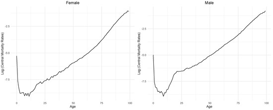
Figure 1.
Logarithm of the central mortality rates of the French population for the year 1994 (longitudinal representation).
On the other hand, the cross-sectional methodology we adopt (following the pioneering work of [17]) is justified, given that we examine events that have an impact across all age groups. Notably, we emphasize positive factors, such as improvements in socio-economic living conditions over time, advances in medical technology, enhanced quality of healthcare services, and the proliferation of healthcare facilities. Moreover, global issues, such as climate change, which leads to extreme events and other catastrophic situations, can have a widespread influence on the French population, thereby increasing mortality risk.
The phenomenon described exhibits a significant declining pattern during the period under examination, as depicted in Figure 2. Across nearly all age groups, male central mortality rates surpass those of females, with distinct variations in all of the age brackets under consideration. Moreover, in this manuscript, we segmented every temporal sequence concerning the historical central mortality rates of the French population into two subgroups: one for modeling and estimation, covering the years from 1940 to 2009, and another for forecast validation, spanning the years from 2010 to 2020. The process described above is commonly known in mathematics and statistical modeling as “Hold-out”. The “Hold-Out” process involves dividing a data set into two subsets: the training set (1940–2009) and the test set (2010–2020). The training set is used to train and build the model, while the test set is held out and not used during the training phase. Instead, it is used to evaluate the model’s performance after training. This approach has many applications, including also being used for mortality modeling (see [11]).
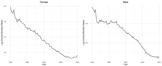
Figure 2.
Logarithm of the central mortality rates of individuals aged 64 over time (cross–sectional representation).
This manuscript is organized in the following manner: In Section 2, we utilize both the geometric Brownian motion and the stochastic Gompertz model to analyze French mortality data (central mortality rates) for the purpose of deriving model estimations and forecasts. Additionally, we delve into the statistical elements of parameter estimation and validation for both models, concluding with a model comparison to determine the most suitable one for forecasting French central mortality rates. Furthermore, in the final part of this section, we perform a comparative study between the results obtained from these SDE models when they were fitted to the Portuguese central mortality rates (the results regarding this application are stated in [18]). Additionally, the primary findings and conclusions of this study are outlined in Section 3.
2. Stochastic Differential Equation Models Fitted to Central Mortality Rates
2.1. The Geometric Brownian Motion and the Stochastic Gompertz Model
The geometric Brownian Motion (briefly, GBM), also referred to as the Black–Scholes model, holds significant recognition in the financial community. It stands out as the predominant model for characterizing the dynamics of a particular stock price on the stock exchange and other economic variables. Notable references include [19,20].
The GBM is characterized by two parameters, r and , which signify, respectively, the arithmetic mean rate of return and the volatility of a given stock price over time. The stochastic differential equation (SDE) that represents the GBM is as follows:
In this equation, signifies the price of a specific stock at a time t, while represents the value of the standard Wiener process at the same moment in time. It is worth noting that this equation finds applications beyond stock prices since it can also be employed to model diverse phenomena, such as population growth, as demonstrated in references such as [21,22], as well as various other variables across different scientific domains. The solution to Equation (1), by applying Itô’scalculus, is:
In this paper, we make the assumption that the observed central mortality rates of the French population follow a GBM. Additionally, we will henceforth use the notation to signify the central mortality rate for an individual of a specific age and sex during the time periods considered in this study. We also assume that the initial observed value is known and independent of the Wiener process. By defining and applyingItô’sformula to , we obtain
Here, let . Moreover, within this study, the parameters R and of the GBM signify, respectively, the mean rate of growth of and the influence of the stochastic environmental variations on mortality dynamics.
The solution for Equation (3) is given by
which follows a Gaussian distribution with an expected value and variance , that is,
In this context, follows a log-normal distribution, where the expected value is given by . Hence, Equation (4) can be expressed in its initial format as:
Moving on to the second model applied in this work, the stochastic Gompertz model (SGM), a deterministic model serving as an illustration for the Gompertz model fitted to central mortality rates may be depicted as
In this context, denotes the dynamic central mortality rate of a specific demographic group characterized by age and sex. Furthermore, a signifies the asymptotic central mortality rate, while b represents the rate at which mortality approaches its asymptotic value, as described in [21].
For simplification purposes, let us introduce the notations and . This allows us to derive a tantamount equation from (6) as
Following [23], to obtain the stochastic Gompertz model (briefly, SGM), we introduce into (7) a stochastic element, , such that . The standard Wiener process, represented as with a parameter , encapsulates the cumulative impact of “environmental” disturbances on the mortality dynamics up to a time t. Parameter quantifies the degree of environmental variability resulting from random disruptions that affect the variable and deviate it from its dynamic trend. Consequently, we can derive the autonomous SDE
where denotes the known original value, a (with ) represents the logarithm of the average rate of asymptotic mortality, b signifies the velocity of approximation to the asymptotic value, and expresses the intensity of random environmental fluctuations.
The solution of (8), by applyingItô’scalculus, is
Taking into consideration that , we obtain
and considering its expected value and variance, yields
2.2. Estimation
For the case of the GBM, from Equation (5), and following [21], we derive the p.d.f of , , expressed as
Let us consider the presence of the subsequently ordered pairs of observation instances and observed values where k ranges from 0 to n, and . Additionally, let us assume that denotes the years in which the French central mortality rates were recorded for each age and sex, where n corresponds to the final year of observed French central mortality rates. Under these conditions, the p.d.f. of given is given by:
assuming that .
Moreover, when we take into account the parameter vector , we can derive the maximum likelihood function for (9), expressed as:
Additionally, we can derive the explicit expressions for the maximum likelihood estimators of p, as detailed in [21], by solving the ensuing system of equations
deriving, for ,
and
Since, in this work, the central mortality rates for the French population are represented on an annual basis, we can make the reasonable assumption that . This simplification greatly streamlines the calculations, and it is applicable to both SDE models fitted to the mortality data of the French population and demonstrated in the subsequent subsections.
To construct confidence intervals for parameters R and V, we can explore the asymptotic properties of the maximum likelihood estimators. As illustrated in [24], the Fisher information matrix for this case is
On the other hand, the variance of each one of the parameters in is given by the diagonal values of the inverse of F, represented as matrix H,
For both parameters within p, we manage to approximate the confidence interval bounds based on a confidence level of , where . The corresponding asymptotic confidence intervals for both parameters within p are as follows:
and
where represents the quantile associated with the probability from the normal distribution. In this scenario, it is also possible to calculate the exact confidence intervals, denoted as , using the exact distributions, as detailed in [21]. These distributions are defined as:
and
In this context, and denote the t-Student and Chi-squared distributions, each with degrees of freedom. Consequently, the precise confidence intervals for both R and V are computed through the following formulas:
and
In this specific scenario, and signify the quantiles corresponding to the probability in the t-Student and Chi-squared distributions, respectively, each with degrees of freedom.
Given that we possess the observed values of the central mortality rates for the French population (across various ages and sexes) until a specific time instance denoted as , and one of the principal objectives of this study is to elucidate the forthcoming trajectory of the French central mortality rates using SDE models, the subsequent task involves generating forecasts for the time period . Let us assert that is a Markov process. Hence,
and, from (9), one obtains
For long-term (LT) forecasts concerning each age and sex and for time instances , we can adopt the following approach,
In the given context, signifies the approximated value of the mathematical expectation. Since the real value of R remains unknown, we substitute it with .
The step-by-step (SS) forecasts are generated employing a logic akin to the one employed in deriving (10). However, at each time step, which, in our case, corresponds to one year, we update t, the latest observed value, and the parameter estimates. This approach ensures that our forecasts evolve dynamically as we progress through time.
As we are dealing with random variables, we turn to Monte Carlo simulations to approximate the forecasting error distribution, , and ascertain the forecasting confidence intervals. Utilizing Equation (9), we compute the mean and variance of . Employing maximum likelihood estimates for p, we simulate a sufficiently large number of trajectories, denoted as S (in this case, ), represented by the vector , for each age and sex. This process allows us to obtain, up to a specific year , a new parameter vector for each of the S simulated replicas. Additionally, we obtain forecasts denoted as (for ), along with the corresponding forecast errors, . Furthermore, we compute the empirical mean and variance of these errors across a set of S replicas. These computed values are subsequently utilized to estimate the mean and variance of the forecasting errors.
Let and denote the respective empirical expected values and variances. Subsequently, we can derive an approximation, denoted as , for for a specific age and sex, expressed as:
In the case of the SGM and following the analogous rationale for the GBM, let us assume that and designate as the years during which the central mortality rates of the French population were recorded. The transient p.d.f. of is then:
where
and
The parameter vector can be estimated using the maximum likelihood method as well. Consequently, we obtain,
In order to obtain , one must compute
Fixing (as seen in [21]), we obtain
and
Without loss of generality, let us suppose that , as we are examining the annual central mortality rates of the French population sourced directly from [15]. Based on the equations presented earlier, we can define as a function of , denoted as . Additionally, we can define as a function of both and , expressed as . Consequently, we establish a new function denoted as , possessing identical optimal values to those defined in Equation (11) and relying exclusively on the parameter b,
where .
For each age bracket and both sexes, we ascertain the maximum likelihood estimator of b by minimizing the symmetric form of through the use of the R function titled . This approach, outlined in [25] and put into practice in [21], employs instead of to compute the maximum likelihood estimators for the parameter vector . This method proves particularly advantageous when explicit expressions for the estimators are challenging to derive, offering the primary benefit of computational efficiency. Once is obtained, we can determine the maximum likelihood estimators and using the expressions and .
Given that we possess values related to the French population’s central mortality rates up to a specific time and that one of our main objectives is to compute forecasts for a future time t, where , and considering the Markovian nature of the process, it follows that,
where . For long-term (LT) forecasts, taking into account each age and sex, we can employ the following approach,
Here, represents an approximation of the mathematical expectation, with the exact values of A and b being replaced by and .
The SS forecasts are computed using a similar method described in Equation (12). Nonetheless, with each step forward in time (one year), we update not only the last observed value but also the values of t and of the parameter estimates.
2.3. Results
We used the GBM in order to fit the observed central mortality rates of the French population, separately for each age bracket (ages 0 to 99) and for each sex. In this analysis, we employed the variable , where symbolizes the expected central mortality rate at a time t, and represents the initial observed central mortality rate of an individual.
In Figure 3 and Figure 4, you can see the estimated model parameters: and . These parameters correspond to distinct estimates for each age and gender. The figures also display the asymptotic confidence intervals denoted as and the exact confidence intervals marked as associated with each parameter. Upon examining the patterns exhibited by the estimated parameters, we observe that exhibits a mild growing trend; in particular, it becomes more pronounced after the initial ages studied and increases notably after age 20. Additionally, it can also be seen that in the case of males, parameter exhibits a sharp decrease in its value when reaching age 20. This sharp decrease is most likely linked to the increased volatility registered in the central mortality rates of young males, which is a consequence of the increased uncertainty related to the survival of young male soldiers in World War II. Furthermore, it is worth noting that while the estimated parameter demonstrates a consistent increasing trend with respect to the individual’s age, The aforementioned does not apply to . The latter exhibits additional pronounced variations across different age groups, with notable variations when examining ages between 0 and 40 and beyond age 90, especially within the male population. This presents a distinct pattern compared to . Regarding the confidence intervals, both of them ( and ) were computed using a 95% confidence level. For both parameters, and exhibit nearly identical values (as depicted in Figure 3 and Figure 4, where the representations of both confidence intervals closely align across most ages and both sexes). Therefore, there are no substantial advantages associated with using exact confidence intervals () in this study.
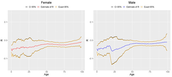
Figure 3.
Estimates , , and for the GBM.
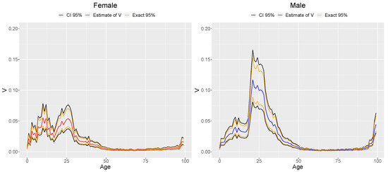
Figure 4.
Estimates , , and for the GBM.
The range in confidence intervals for R and V is roughly proportional to and V, respectively. This relationship accounts for the larger range in the confidence intervals for R when compared to those for V. Additionally, concerning R, it elucidates the notably wider confidence intervals observed when analyzing male individuals aged between 10 and 40 years and those aged 90 or older.
Results pertaining to model estimations and central mortality rate forecasts were reverted to their original scale, denoted as , instead of the transformed variable . In Figure 5, you can observe the central mortality rate’s model estimations (with in Equation (4) and with the model’s parameters replaced by their maximum likelihood estimates) and forecasts for a 65-year-old male.

Figure 5.
GBM model estimations (top) and forecasts (bottom) for a 65 year old male.
We would like to emphasize that we utilized the observed central mortality rates for the years from 1940 to 2009 in our calibration process, reserving the subsequent years (from 2010 to 2020) to perform forecast validations. Moreover, we opted to present these values in Figure 5 (top) in relation to model estimations and forecasts. This inclusion serves to offer additional insight beyond the error estimate, as it enables a comparison of the model’s predictions against observed trends. In general, the outcomes derived from the application of the GBM are highly favorable, as the model adeptly captures the observed central mortality rates’ behavior, replicating the declining trend observed over the last few decades and providing valid forecasts.
Moreover, to assess the “goodness of fit" for these values, we employed the Mean Squared Error (MSE) as a quantitative measure. When conducting a comprehensive analysis of the results, it becomes evident that both model estimations and forecast values exhibit a superior fit (as per the aforementioned criterion) within the data series associated with the female gender. In Appendix A, specifically in Figure A1, Figure A2 and Figure A3, we provide visual representations of the MSE values for each age and gender, for model estimations, and for both the LT and SS forecasting methods.
The contrast in the model’s performance between sexes becomes increasingly pronounced after the age of 90. In this age group, for both sexes (with the difference being more pronounced in males), the model struggles to capture the variations in the central mortality rates’ time series and fails to provide a satisfactory model estimate. This accounts for the sharp rise in MSE values, as depicted in Figure A1.
Similar to the first part of Section 2.3, related to the GBM, we fitted the stochastic Gompertz model (SGM) to the French population’s central mortality rates, considering each age within the range from 0 to 99 years for both sexes. To achieve this, we specifically employed the variable .
Figure 6 provides a visual representation of the SGM parameters, a, b, and , for the various age groups considered in this manuscript. It is important to note that while we estimated the value of A as , we opted to present the parameter in its original scale, denoted as a, signifying the average asymptotic central mortality rate (geometric mean). Additionally, within the same figure, we showcase the SGM parameter values, excluding the last 10 age groups. These plots are easily distinguishable, as the age axis ranges from 0 to 100 in the first case and from 0 to 90 in the second case. This extended age range allows for a more detailed examination of the parameter behavior in adult ages and aids in comprehending the patterns observed in each graph, particularly for the case of parameter b.

Figure 6.
SGM parameter estimates (a, b, and ) for each age and sex.
Indeed, the outcomes concerning the model’s estimated parameters align with expectations, given the insights gathered from prior research projects and articles focused on the subject of human mortality. Consequently, parameter a exhibits an increase in relation to the individual’s age, with markedly increased values observed when examining the later ages within the lifespan curve, where the likelihood of mortality is significantly higher.
Parameter b exhibits an initial upward trajectory when examining the early ages within the lifespan curve, followed by a significant surge around age 20, which is particularly noticeable in males. Subsequently, it shows a declining trend between ages 21 and 70. After reaching age 90, the estimated values of b experience a substantial increase, reaching approximately 1.5 for males and 0.4 for females.
Regarding , which represents the parameter associated with the stochastic integral term of the model in question, measuring the degree of random environmental fluctuations affecting observed mortality rates, the following observations can be made: The estimated values demonstrate an upward trend in the younger age groups analyzed, particularly among children and young adults who were significantly affected by World War II, primarily due to conscription. Beyond age 35, there is a marked reduction in these values, with a relatively stable pattern observed between the ages of 55 and 90. However, in the later stages of the lifespan curve, there is a renewed upward trend in the parameter, reflecting the vulnerability of the elderly individuals analyzed, for whom any random event may result in the death of the individual.
Additionally, Figure 6 indicates a more pronounced variability in the parameter estimates of b and between successive age groups, in contrast to parameter a. When examining the trend of these estimates in relation to age, it becomes apparent that, while both sexes exhibit similar patterns, the estimated values are consistently higher in males than in females across all parameters.
In Figure 7, we illustrate the model estimations of the central mortality rates (obtained by setting and substituting the model parameters with their maximum likelihood estimates) and the forecasts for a 65-year-old female.

Figure 7.
SGM model estimations (top) and forecasts (bottom) for a 65 year old female.
In broad terms, the outcomes of implementing the SGM exhibit a favorable performance. Both the model estimations and subsequent forecasts tend to perform notably better in the female sex, although the disparity in the model’s performance between sexes is less conspicuous compared to the GBM. This distinction becomes more pronounced after the age of 80, as evident in Figure A4, Figure A5 and Figure A6 seen in Appendix A. Thus, similar to the previous subsection concerning the GBM, the SGM appears to be a suitable choice for modeling this type of data, given the promising results obtained thus far.
2.4. Comparing the Results from Both Models
From the results obtained so far, in the following subsections, we juxtapose the outcomes of the two SDE models utilized in the preceding subsections: the GBM and the SGM.
Our conclusion is that both models provide reasonable forecasts, showing values within a comparable order of magnitude and with nearly identical MSEs. This preliminary analysis does not provide sufficient evidence to unequivocally favor one model over the other. Figure 8 demonstrates the application of both stochastic differential equation models for individuals aged 20, regardless of gender (the results are displayed in their original data scale).
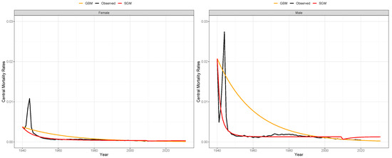
Figure 8.
Comparison between the GBM and SGM model estimations with LT forecasts for the age 20 and for both sexes (Female on the left side, Male on the right side).
For the majority of age groups and both sexes, the model’s estimations tend to resemble the left side of Figure 8. This resemblance is attributed to the declining exponential pattern in observed central mortality rates, which is a consequence of the high central mortality rates recorded in the 1940s during World War II. This effect is more noticeable when analyzing the decreasing central mortality rates’ trend in males. It is important to note that the curve predicted by the GBM primarily tracks fluctuations in the series towards the end of the model estimation period, whereas the SGM effectively captures the variability of the series from the beginning of the analyzed time period, starting in 1940.
Regarding the forecast for the time period between 2010 and 2020, it is noticeable that, for the majority of age groups, the GBM tends to underestimate with a declining trend, whereas the SGM tends to overestimate with a rising trend, as illustrated in Figure 8.
While the performance of each model distinctly differs from the other, it becomes evident when we analyze the disparity in their individual MSE for each age group and sex, that the GBM presents advantages over the SGM when computing LT and SS forecasts (except for newborns and individuals aged between 60 and 74), whereas, for computing model estimations, the SGM outperforms the GBM in almost all of the age brackets (with the exception of females aged between 25 and 30 years old and males aged between 60 and 74 years old).
Figure A7 through Figure A12, available in Appendix A, illustrate the disparities in the MSE between the GBM and SGM models, meaning , across all age groups and for each sex. It is worth noting that to enhance visibility, the differences are scaled by a factor of 10.000 due to the small and closely matched error estimates in terms of magnitude for several age groups.
2.5. Comparative Study between the Model’s Results: France Versus Portugal
As it was stated in Section 1, two main goals of this work are to compare the mortality dynamics of the French and Portuguese populations and also to compare the results obtained when SDE models are fitted to the central mortality rates of these countries, taking into account the results obtained in [18]. When analyzing Figure 9, we can state that for young individuals (20 years old) of both sexes, the French central mortality rates are higher during the time period between 1940 and 1950 than those related to the Portuguese population. This situation occurs due to the fact that most young French men were drafted during World War II, leading to a spike in the French central mortality rates during this time horizon. The same does not occur when we analyze the Portuguese central mortality rates since Portugal stayed neutral in this war. Moreover, we can see that, for older individuals (aged 64), the mortality rates present almost similar values, meaning that the effects of this war did not have a significant impact on the central mortality rates of older individuals.

Figure 9.
Central mortality rates of the French and Portuguese populations for individuals aged 20 years old (top) and for individuals aged 64 years old (bottom).
When comparing the results of the application of SDE models (the GBM and SGM) to the central mortality rates of France and Portugal, we can state that both models present realistic model estimations and forecasts that manage to replicate the decreasing central mortality rates trend recorded in the last few decades for both of these countries. However, as we have seen previously in Section 2.4, in the case of the French population’s central mortality rates, the GBM outperforms the SGM when computing LT and SS forecasts (except for newborns and individuals aged between 60 and 74), whereas, for computing model estimations, the SGM outperforms the GBM in almost all of the age brackets (with the exception of females aged between 25 and 30 years old and males aged between 60 and 74 years old). Meanwhile, for the case of the Portuguese population’s mortality rates, in the context of both the SS and LT forecasts, the GBM prevails over the SGM in the majority of age groups for both sexes, as indicated by the differences in MSEs between the models. In fact, even when only considering the model’s estimations, the GBM in most age groups outperforms the SGM, with the exception of individuals aged 80 or more years for both sexes. This difference in the model’s performances between these two countries is most likely due to the significant spike in the French central mortality rates (particularly in younger individuals) in the 1940s, which leads the SGM to outperform the GBM since the SGM managed to capture the variability of the series at the beginning of the time period under analysis (meaning 1940).
3. Conclusions
It is reasonable to infer that the application of SDE models, such as the GBM and SGM, closely reproduces the observed trend of declining central mortality rates in the French population. Additionally, both models yield forecasts that align closely with the historical data, featuring values of similar magnitude and relatively low MSEs. This balance in forecast accuracy prevents us from conclusively determining the superiority of one model over the other.
Nonetheless, in Section 2.4, when we conducted a comparative analysis of the model’s results, it became evident that the GBM demonstrated superior performance over the SGM when computing LT and SS forecasts (except for newborns and individuals aged between 60 and 74), whereas, for computing model estimations, the SGM outperforms the GBM in almost all of the age brackets (with the exception of females aged between 25 and 30 years old and males aged between 60 and 74 years old).
As expected, SS forecasts exhibit a smaller prediction error in comparison to the LT forecasts. This is a natural outcome, considering that in the case of SS forecasts, we continuously update the time variable t, the most recent observed value, and the parameter estimates as we advance one step through time. In other words, SS forecasts benefit from increased accuracy due to the additional and current information used, making them inherently more precise than LT forecasts.
Additionally, when we compare the model’s performance between the French and Portuguese central mortality rates, we can state that the SGM outperforms the GBM in the French case (when considering only model estimations) while the opposite occurs when dealing with the application of these models for the central mortality rates of the Portuguese population.
In conclusion, our primary objective was to elucidate the mortality trends within the French population, and we have observed that the methodology applied has yielded promising results. However, we acknowledge the possibility of one or more unidentified variables that may influence the likelihood of death in various groups of individuals, regardless of age or sex, during specific time periods. We believe that enhancing this model requires extracting more valuable insights from population data, enhancing parameter estimation flexibility, and ultimately elevating its general performance.
Furthermore, as the data set related to the central mortality rates of the French and Portuguese populations used in this manuscript only encompasses the year 2020 amidst the COVID-19 pandemic, it is essential to acknowledge that future research might yield different results if a broader time horizon, encompassing mortality data from the years 2021 and 2022, is considered. We anticipate recalculating our results once the Human Mortality Database updates its mortality data to assess any significant variations.
Additionally, all the results presented in this work were computed using the R programming language, and the corresponding R code is available upon request to the authors.
Author Contributions
Validation, N.M.B.; writing—original draft, D.d.S.B.; writing—review & editing, N.M.B.; supervision, N.M.B. All authors have read and agreed to the published version of the manuscript.
Funding
Nuno M. Brites was partially supported by the projects (i) CEMAPRE/REM–UIDB/05069/2020 and (ii) EXPL/EGE-IND/0351/2021, both funded by FCT/MCTES through national funds.
Data Availability Statement
Data available on request due to privacy restrictions.
Acknowledgments
We wish to thank the Editor and two anonymous Reviewers for their discussions and comments, which improved the quality of our manuscript.
Conflicts of Interest
The authors declare no conflict of interest.
Abbreviations
| SDE | stochastic differential equation |
| SS | Step-by-Step |
| LT | Long-Term |
| SGM | stochastic Gompertz model |
| GBM | geometric Brownian motion |
| p.d.f | probability density function |
| MSE | Mean Squared Error |
Appendix A
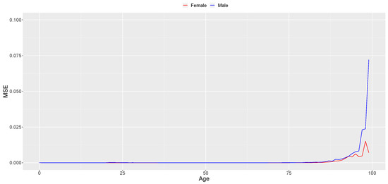
Figure A1.
Mean Squared Error (MSE) of the GBM central mortality rate’s model estimations (1940–2020).

Figure A2.
Mean Squared Error (MSE) of the GBM LT forecasts (2010–2020).
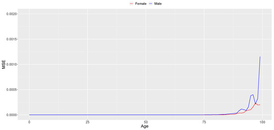
Figure A3.
Mean Squared Error (MSE) of the GBM SS forecasts (2010–2020).
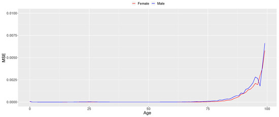
Figure A4.
Mean Squared Error (MSE) of the SGM central mortality rate’s model estimations.
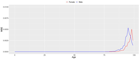
Figure A5.
Mean Squared Error (MSE) of the SGM LT forecasts (2010–2020).
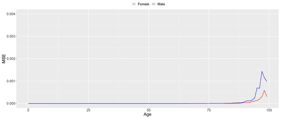
Figure A6.
Mean Squared Error (MSE) of the SGM SS forecasts (2010–2020).

Figure A7.
Difference (×10,000) between the Mean Squared Errors (MSEs) associated with the central mortality rate’s model estimations of the GBM and SGM, female sex.

Figure A8.
Difference (×10,000) between the Mean Squared Errors (MSEs) associated with the central mortality rate’s model estimation of the GBM and SGM, male sex.

Figure A9.
Difference (×10,000) between the Mean Squared Errors (MSEs) associated with the SS forecasts (from 2010 to 2020) of the GBM and SGM, female sex.

Figure A10.
Difference (×10,000) between the Mean Squared Errors (MSEs) associated with the SS forecasts (from 2010 to 2020) of the GBM and SGM, male sex.

Figure A11.
Difference (×10,000) between the Mean Squared Errors (MSEs) associated with the LT forecasts (from 2010 to 2020) of the GBM and SGM, female sex.

Figure A12.
Difference (×10,000) between the Mean Squared Errors (MSEs) associated with the LT forecasts (from 2010 to 2020) of the GBM and SGM, male sex.
References
- Lee, R.D.; Carter, L.R. Modeling and Forecasting U.S. Mortality. J. Am. Stat. Assoc. 1992, 87, 659–671. [Google Scholar] [CrossRef]
- Booth, H.; Maindonald, J.; Smith, L. Applying Lee-Carter under Conditions of Variable Mortality Decline. Popul. Stud. 2002, 56, 325–336. [Google Scholar] [CrossRef] [PubMed]
- Renshaw, A.; Haberman, S. Lee-Carter Mortality Forecasting with Age-Specific Enhancement. Insur. Math. Econ. 2003, 33, 255–272. [Google Scholar] [CrossRef]
- Plat, R. On stochastic mortality modeling. Insur. Math. Econ. 2009, 45, 393–404. [Google Scholar] [CrossRef]
- Shryock, H.S.; Siegel, J.S. CHAPTER 23—Population Projections. In The Methods and Materials of Demography; Shryock, H.S., Siegel, J.S., Eds.; Studies in Population, Academic Press: San Diego, CA, USA, 1976; pp. 439–482. [Google Scholar] [CrossRef]
- Booth, H.; Tickle, L. Mortality Modelling and Forecasting: A Review of Methods. Ann. Actuar. Sci. 2008, 3, 3–43. [Google Scholar] [CrossRef]
- Aro, H.; Pennanen, T. A user-friendly approach to stochastic mortality modelling. Eur. Actuar. J. 2011, 1, 151–167. [Google Scholar] [CrossRef]
- Lagarto, S.; Braumann, C.A. Modeling Human Population Death Rates: A Bi-Dimensional Stochastic Gompertz Model with Correlated Wiener Processes. In New Advances in Statistical Modeling and Applications; Pacheco, A., Santos, R., Oliveira, M.d.R., Paulino, C.D., Eds.; Springer International Publishing: Cham, Switzerland, 2014; pp. 95–103. [Google Scholar]
- Villegas, A.M.; Kaishev, V.K.; Millossovich, P. StMoMo: An R Package for Stochastic Mortality Modeling. J. Stat. Softw. 2018, 84, 1–38. [Google Scholar] [CrossRef]
- Agadi, R.P.; Talawar, A.S. Stochastic differential equation: An application to mortality data. Int. J. Res. 2020, 8, 229–235. [Google Scholar] [CrossRef]
- Atance, D.; Debón, A.; Navarro, E. A Comparison of Forecasting Mortality Models Using Resampling Methods. Mathematics 2020, 8, 1550. [Google Scholar] [CrossRef]
- Alonso-García, J. AAS Thematic issue: “Mortality: From Lee–Carter to AI”. Ann. Actuar. Sci. 2023, 17, 212–214. [Google Scholar] [CrossRef]
- Pitacco, E. Survival models in a dynamic context: A survey. Insur. Math. Econ. 2004, 35, 279–298. [Google Scholar] [CrossRef]
- Atance, D.; Balbás, A.; Navarro, E. Constructing dynamic life tables with a single-factor model. Decis. Econ. Financ. 2020, 43, 787–825. [Google Scholar] [CrossRef]
- Human Mortality Database. University of California and Max Planck Institute for Demographic Research. 2023. Available online: http://www.mortality.org (accessed on 15 April 2023).
- Heligman, L.; Pollard, J.H. The age pattern of mortality. J. Inst. Actuar. 1980, 107, 49–80. [Google Scholar] [CrossRef]
- Lagarto, S. Modelos Estocásticos de Taxas de Mortalidade e Aplicações. Ph.D. Thesis, Universidade de Évora, Évora, Portugal, 2014. [Google Scholar]
- Baptista, D. Stochastic Differential Equations Death Rates Models: The Portuguese Case. Master’s Thesis, Instituto Superior de Economia e Gestão, 2022. Available online: http://hdl.handle.net/10400.5/26200 (accessed on 15 April 2023).
- Black, F.; Scholes, M. The Pricing of Options and Corporate Liabilities. J. Political Econ. 1973, 81, 637–654. [Google Scholar] [CrossRef]
- Garcin, M.; Grasselli, M. Long versus short time scales: The rough dilemma and beyond. Decis. Econ. Finan 2022, 45, 257–278. [Google Scholar] [CrossRef]
- Brites, N.M. Modelos Estocásticos de Crescimento Individual e Desenvolvimento de Software de Estimação e Previsão. Master’s Thesis, Universidade de Évora, Évora, Portugal, 2010. Available online: http://hdl.handle.net/10174/19943 (accessed on 15 April 2023).
- Panik, M. Stochastic Differential Equations: An Introduction with Applications in Population Dynamics Modeling; John Wiley & Sons, Inc.: Hoboken, NJ, USA, 2017. [Google Scholar]
- Brites, N.M.; Braumann, C.A. Harvesting in a Random Varying Environment: Optimal, Stepwise and Sustainable Policies for the Gompertz Model. Stat. Optim. Inf. Comput. 2019, 7, 533–544. [Google Scholar] [CrossRef]
- Casella, G.; Berger, R. Statistical Inference, 2nd ed.; Duxbury: New Dehli, India, 2002. [Google Scholar]
- Franco, J. Maximum Likelihood Estimation of Mean Reverting Processes; Real Options Practice; Ownward Inc.: Houston, TX, USA, 2003. [Google Scholar]
Disclaimer/Publisher’s Note: The statements, opinions and data contained in all publications are solely those of the individual author(s) and contributor(s) and not of MDPI and/or the editor(s). MDPI and/or the editor(s) disclaim responsibility for any injury to people or property resulting from any ideas, methods, instructions or products referred to in the content. |
© 2023 by the authors. Licensee MDPI, Basel, Switzerland. This article is an open access article distributed under the terms and conditions of the Creative Commons Attribution (CC BY) license (https://creativecommons.org/licenses/by/4.0/).