
Stability of Vertical Rotations of an Axisymmetric Ellipsoid on a Vibrating Plane

Ural Mathematical Center, Udmurt State University, Izhevsk 426034, Russia
*
Author to whom correspondence should be addressed.
Mathematics 2023, 11(18), 3948; https://doi.org/10.3390/math11183948
Submission received: 20 August 2023
/
Revised: 12 September 2023
/
Accepted: 14 September 2023
/
Published: 17 September 2023
(This article belongs to the Section Dynamical Systems)
Abstract
:In this paper, we address the problem of an ellipsoid with axisymmetric mass distribution rolling on a horizontal absolutely rough plane under the assumption that the supporting plane performs periodic vertical oscillations. In the general case, the problem reduces to a system with one and a half degrees of freedom. In this paper, instead of considering exact equations, we use a vibrational potential that describes approximately the dynamics of a rigid body on a vibrating plane. Since the vibrational potential is invariant under rotation about the vertical, the resulting problem with the additional potential is integrable. For this problem, we analyze the influence of vibrations on the linear stability of vertical rotations of the ellipsoid.
Keywords:
axisymmetric ellipsoid; vibrating plane; nonholonomic constraint; permanent rotations; vertical rotations; stability; vibrational potential; integrabilityMSC:
37N05; 70E18; 70E50; 70K201. Introduction
In this paper, we consider the dynamics of an ellipsoid of revolution with axisymmetric mass distribution on an absolutely rough plane. We assume that the supporting plane performs periodic motions. The analysis of rigid body dynamics on a moving plane is motivated by problems of modeling the motion of a rigid body under various external influences, for example, inside a moving vehicle. The modeling of this motion usually involves oscillations or rotations of the supporting surface, which are considered as such external influences. In this paper, we focus on vertical vibrations of the supporting plane.
The problem of the motion of a rigid body on a moving plane goes back to the classical problem of the Kapitsa pendulum [1,2,3,4], a mathematical pendulum with a vibrating suspension point. This is one of the simplest problems demonstrating the dynamical stability: under sufficiently fast oscillations of the suspension point the pendulum stabilizes in the upper position, which is unstable in the absence of vibrations. Later, the problems of the motion of rigid bodies rolling on vibrating surfaces were addressed. Without claiming to cite all relevant literature, we mention [5,6,7,8,9,10,11,12]. In particular, [5] examines the motion of a homogeneous sphere on a vibrating surface of complex form. In [6], the dynamics of a rattleback on a vibrating plane is investigated. The authors of [7,8,10] analyze the dynamics of spherical bodies with a displaced center of mass on a vertically vibrating plane. The paper [9] examines the dynamics of a spherical robot with an axisymmetric pendulum on a vibrating plane and, in particular, analyzes the influence of vibrations on vertical rotations of the pendulum. The dynamics of the Chaplygin sphere on a horizontally oscillating plane and the control of its motion using the gyrostatic momentum is studied in [11,12].
One of the efficient approaches to investigating the dynamics of bodies on a vibrating surface is the application of the methods of averaging theory. This approach, which consists of averaging equations over a period, considerably facilitates analysis of the dynamics of bodies on a vibrating plane. Under some restrictions on the oscillation parameters the systems obtained using this approach provide a fairly accurate description of the dynamics of a rigid body on a plane. Using this method, P. L. Kapitsa [2] showed that the oscillations of the suspension point of the pendulum cause a torque whose magnitude is determined only by the mass of the pendulum and by the square of the oscillation velocity of the suspension point. This torque was called by the author the vibrational torque. The procedure of averaging the equations of motion and deriving the vibrational torque is described in detail for a rigid body with a vibrating suspension point in [13]. The recent paper [14] presents a bifurcation analysis of the dynamics of the Lagrange top with an additional vibrational potential that approximately describes the vertical oscillations of the suspension point. The averaging of the equations of motion for a sphere with a displaced center of mass which rolls without slipping on a vibrating plane was performed in [7,10]. In this paper, we perform a similar procedure of averaging for an ellipsoid of revolution rolling on a vibrating plane.
One of the problems treated in this paper is the investigation of the influence of the vibrations of the plane on the stability of partial solutions (vertical rotations) of an ellipsoid. In the case of a fixed supporting plane, the stability of partial solutions of an ellipsoid was widely explored in the literature for bodies rolling with and without slipping. Much effort was directed at analyzing the stability of permanent rotations of geometrically and dynamically symmetric bodies [15,16,17,18]. The ellipsoid of revolution is a special case of such bodies. In [19] the stability of permanent rotations of a homogeneous triaxial ellipsoid on a smooth plane was investigated. Permanent rotations of an ellipsoid with axisymmetric mass distribution on a smooth plane were analyzed in detail in [20]. The paper [21] also analyzes permanent rotations of an ellipsoid of revolution on a smooth plane, but from the viewpoint of the problem of elevation of Jellett’s egg (see also [22]). This paper explores the influence of the form of an (oblate or prolate) ellipsoid and the displacement of the center of mass on the possibility of lifting it to the vertical position by means of dissipative forces. In [22], only the prolate ellipsoid is considered.
The problem of an ellipsoid moving on an absolutely rough plane, as well as the search for and analysis of permanent rotations, has also received a great deal of attention in the literature. In [23,24], the stability of permanent (including vertical) rotations of an arbitrary convex body of revolution was investigated and conditions for the stability of such rotations were derived. In the work of A. P. Markeev [25,26] on the dynamics of a triaxial ellipsoid, an assumption was made about similarity of the form of the ellipsoid to the form of the sphere. Interesting results of the search for and analysis of permanent rotations were obtained in the work of A. V. Karapetyan [27]. He showed that there exist mass-geometric parameters of the ellipsoid such that it performs permanent rotations about an arbitrary axis passing through the center of mass. A detailed stability analysis of such rotations was made in [28]. The stability of vertical rotations of an axisymmetric ellipsoid about the principal axis which is not an axis of revolution was investigated in [29], where the instability of such solutions was shown. In [30], a parametric analysis of the stability of permanent rotations of a homogeneous triaxial ellipsoid was carried out: stability regions on the parameter plane (the ratios of two semiaxes to the third) were constructed depending on the velocity of rotation. In [31], bifurcation diagrams in the space of first integrals were constructed for a balanced ellipsoid of revolution in the case of a smooth and a rough plane.
In this paper, we study the dynamics of an ellipsoid of revolution on a vertically vibrating absolutely rough plane. The paper is structured as follows. In Section 2, we derive equations of motion for an ellipsoid with a displaced center of mass on a vibrating plane and, by averaging them, obtain the vibrational torque. In Section 3, we present invariants of the system considered and perform a reduction in the equations of motion to a system with one degree of freedom. In Section 4, we investigate the stability of vertical rotations of the ellipsoid and analyze the influence of vibrations of the supporting plane on their stability.
2. Equations of Motion
2.1. Model Assumptions
Consider the motion of a dynamically symmetric ellipsoid of revolution with a displaced center of mass on a horizontal plane performing periodic oscillations. We will examine this problem under the following assumptions:
- The ellipsoid moves with one point in contact with the supporting plane without losing contact with it;
- The velocity of the point of contact P of the ellipsoid with the supporting plane is zero;
- In the general case, the center of mass of the ellipsoid is offset from its geometric center and lies on its symmetry axis;
- The supporting plane performs vertical periodic oscillations according to the law .
2.2. Configuration Space and Kinematic Relations
Consider the motion of a dynamically symmetric ellipsoid of revolution of mass m with semiaxes and on an absolutely rough horizontal plane (Figure 1). Assume that the center of mass of the ellipsoid is offset from its geometric center along the symmetry axis by distance a.
To describe the motion of the ellipsoid, we introduce two coordinate systems:
- –
- A fixed (inertial) coordinate system with unit vectors , where is the vertical unit vector;
- –
- A moving coordinate system with unit vectors attached to the ellipsoid, with origin at its center of mass C and with the axis directed along the symmetry axis.
Referred to the moving frame , the vector of displacement of the center of mass can be written as .
Let us specify the position of the ellipsoid by the coordinates of its center of in the fixed coordinate system, and its orientation in space, by the rotation matrix whose columns are the unit vectors referred to the moving coordinate system:
Hence, the configuration space of the problem of the free motion of the ellipsoid is the product .
By definition, the vectors , , and , which form an orthonormal basis, satisfy the relations
We will describe the dynamics of the system by the vectors of the angular velocity and the velocity of motion of the center of mass and refer these vectors to the moving coordinate system (here and in what follows, unless otherwise specified, all vectors will be referred to the moving coordinate system ). The vectors and are quasi-velocities and are related to the derivatives of the configuration variables by the following kinematic relations:
2.3. Constraint Equations and Dynamical Equations
Let us write the constraint equations corresponding to the assumptions described in Section 2.1. The condition that the ellipsoid must move without loss of contact with the plane involves imposing the following holonomic constraint on the system:
where is the radius vector of the point of contact (see Figure 1), which can be expressed in terms of the vector using the relation
where .
Remark 1.
In the case of an arbitrary axisymmetric surface, the dependence can be represented as
where and are arbitrary functions related to each other by
In the case of the ellipsoid considered here, explicit expressions for , have the form
The condition that there be no slipping at the point of contact is described by the nonholonomic constraint
Remark 2.
In the chosen quasi-velocities, the Lagrangian function of the system, with the holonomic constraint (2) taken into account, has the form
where is the principal central tensor of inertia of the ellipsoid and is the free-fall acceleration.
We write the equations of motion of the system in the absence of external forces in the form of Lagrange equations in quasi-velocities with the constraints [32,33]
where are undefined multipliers which are found from the joint solution of Equation (6) and the time derivative of the constraint (4).
After eliminating the velocity using the constraint Equation (4), the equations of motion (6) reduce to one vector equation
where . Here and in what follows, by the vector we mean its explicit expression (3) written in terms of the vector . From the equation thus obtained it can be seen that the rolling motion on a vertically vibrating plane is similar to that on a fixed plane with time-dependent free-fall acceleration.
Equations (7) and (1), combined with the constraint (4), give a complete description of the dynamics of an axisymmetric ellipsoid on a vibrating horizontal plane.
We note that the equations for and decouple from the complete system and form a closed system of two vector differential equations
2.4. Averaged Equations of Motion
To average the equations of motion and to obtain a vibrational potential, we apply the method employed in [10], which is based on the Boltzmann–Hamel Equations [34]. As quasi-velocities we need to use the angular velocities and the constraints (4). After eliminating the total time derivative, the Lagrangian function takes the form
Next, we introduce the generalized momenta
and the “quasi-Hamiltonian”
The equations of motion in the variables (9) can be written [34] in the quasi-Hamiltonian form
where are new undefined multipliers.
Remark 3.
To derive Equations (10) and (11), we have used the equation for changing the position of the center of mass of the rigid body relative to the moving coordinate system attached to the oscillating plane. In this case, the quasi-velocity is the velocity of the point of contact, also relative to the moving plane.
By choosing the constraints as quasi-velocities, Equation (11) decouples and is used only to find undefined multipliers. This makes it necessary to express and from Equation (10) and the derivative of the constraint Equation (4), which in the chosen variables takes the form
and to substitute them into Equation (11).
After applying the constraint (12), Equation (10), together with one of the kinematic relations (1), take the form
and completely describe the dynamics of the reduced system.
In what follows, we assume that the oscillations of the plane are performed with small amplitude and high frequency . We introduce a “fast” time variable, , and average the resulting system (13) over it in accordance with the Bogolyubov theorem [35] and taking into account . Comparing the result obtained by averaging with the equations of a similar system without vibrations of the plane, we arrive at the conclusion that fast vibrations lead to the appearance of a vibrational potential of the form
where , the average of the squared velocity of the plane’s motion
is a constant depending on the law of oscillations. In the special case of harmonic oscillations
As stated above, we will consider small oscillations of the plane with high frequency. In this case, in accordance with the Bogolyubov theorem, the solutions of the averaged system will be similar to the solution of an exact system on time intervals of order .
We also note that in the case of axisymmetric mass distribution the vibrational potential depends only on the component . Thus, after averaging we have obtained the problem of an axisymmetric ellipsoid rolling on an absolutely rough plane in a potential possessing axial symmetry. The integrability of this problem was established already in [36]. However, in the general case, additional integrals are not expressed in terms of elementary functions.
Next, we derive equations of motion of the averaged system not by using the Boltzmann–Hamel equations, but by adding the resulting vibrational potential to the Lagrangian (5).
The Lagrangian function of the averaged system with the vibrational potential has the form
In this case, the system is subject to the (autonomous) constraint—the condition that there be no slipping at the point of contact
Substituting the resulting Lagrangian function into Equation (6), eliminating the undefined multipliers using the constraint (15), we obtain a reduced system of equations
where the expression
is the vibrational torque.
Thus, Equations (16) and (1), combined with the constraint (15), give an approximate description of the dynamics of an axisymmetric ellipsoid on a vibrating absolutely rough horizontal plane.
For further analysis, we introduce the angular momentum vector
and rewrite Equation (16) in terms of the angular momenta
where the angular velocity is expressed in terms of the angular momentum as .
Equation (18) contain 8 parameters. We rescale the variables and time as
The resulting system of equations depends on five independent dimensionless parameters, which we denote as follows:
The values of the parameter correspond to an “prolate” ellipsoid, and , to an “oblate” one. The boundary values of the parameter correspond either to a thin rod () or to a thin disk (), but these cases correspond to the motion of a body with a sharp edge, so we do not consider them in this paper.
Remark 4.
The scaling transformation (19) is equivalent to choosing units of measurement of dimensional quantities so that the following relations are satisfied:
In what follows, unless otherwise specified, we will perform all calculations for dimensionless quantities.
3. Integrability of the Averaged System (18)
3.1. Invariants
The equations of motion (18) admit the obvious geometric integral
and the energy integral
and preserve the invariant measure with density [37]
In addition, Equation (18) admit two integrals linear in angular momenta which are due to the axial symmetry of the body and to the invariance under rotation about the vertical. Moreover, these integrals do not collapse when vertical oscillations of the supporting plane are added in explicit form, i.e., Equation (8) also preserve two first integrals, linear in angular momenta , and the invariant measure (21). For the case of an ellipsoid rolling on an absolutely rough plane, these integrals are not expressed in terms of elementary functions.
The equations of motion (18) also possess the symmetry field
which corresponds to invariance of the system under rotations about the axis of dynamical symmetry of the ellipsoid.
3.2. Reduction by the Symmetry Field
Following [37], we choose as new variables the integrals of the vector field (22) in the form
where is the height of the geometric center of the ellipsoid, , and the symbol is introduced to abbreviate some of our formulae.
In the new variables , , and the equations of motion describing the dynamics of the system take the form
where , is the potential energy of the system.
To reconstruct the dynamics of the system (18), it is necessary to add to Equations (24)–(27) a quadrature for the angle of proper rotation . The function with two arguments calculates the arctan value of the quotient of its arguments and takes into account their signs in determining the value of the function in the interval .
3.3. Additional Integrals of Motion and Reduction to a System with One Degree of Freedom
In addition to the energy integral (28), Equations (24)–(27) admit two first integrals of motion. To find them, we divide Equations (25) and (26) by (24) and obtain a system of two linear nonautonomous first-order equations
The general solution of this system of equations can be represented as
where , is the matrix of the fundamental solutions of the system (29) with initial conditions , and are constants of integration that are the required first integrals. As a result, the first integrals of motion have the form
and are functions linear in momenta, with coefficients that are nonalgebraic functions of .
As is well known [20], the problem of an ellipsoid of revolution with a displaced center of mass that moves on a smooth plane admits two additional integrals of motion: the area integral and the Lagrangian integral . Analyzing the expressions (23) for defining , and the chosen initial conditions of the matrix of the fundamental solutions and comparing them with the integrals in the case of a smooth plane, one can conclude that the integral is an analog of the area integral and is an analog of the Lagrangian integral.
Remark 5.
Similar integrals in the case of a body of revolution moving on a smooth plane or in the case of a rubber body rolling on a plane are described by elementary functions. In the problem of a body of revolution rolling on an absolutely rough plane, the first integrals are expressed in elementary functions probably only in the case of a sphere with axisymmetric mass distribution [38]. In the case of a balanced axisymmetric disk, additional integrals are expressed in terms of hypergeometric functions [39,40], and in the case of a balanced ellipsoid of revolution, in terms of the Heun functions [31].
After fixing the level set of the first integrals and , we obtain a system with one degree of freedom
which preserves the energy integral
In this case, in the expressions (31) and (32) the variables and are expressed in terms of the integrals , and the variable using (30).
Remark 6.
After rescaling time as the system (31) becomes Hamiltonian.
Figure 2 shows an example of the phase portrait of the system (31). As can be seen from the figure, for the chosen parameters the phase portrait has three fixed points. Depending on the parameters, the number of fixed points can decrease or increase. Moreover, even in the case of an absolutely smooth plane and in the absence of any additional forces (except for the force of gravity), the bifurcation diagram of the system is a rather complicated surface in the 3-dimensional space of first integrals. The sections formed by the intersection of this surface with a plane corresponding to a fixed value of one of the integrals can be very diverse [20]. Thus, the bifurcation analysis of the system considered here is a challenge in its own right beyond the scope of this paper. In this paper, we will not present a detailed classification of diagrams for the system under consideration, but only analyze the stability of vertical rotations.
4. Vertical Rotations and Analysis of Their Stability
4.1. Vertical Rotations of an Ellipsoid
As is well known [40], for any body of revolution there exist two partial solutions which correspond to vertical rotations of the body about the symmetry axis. By vertical rotations we mean rotations under which the symmetry axis of the ellipsoid is vertical and fixed and the body itself rotates about this axis. By upper vertical rotations we mean rotations under which the center of mass lying on the symmetry axis is above the geometric center of the ellipsoid (this case corresponds to ), and by lower vertical rotations we mean rotations under which the center of mass is below the geometric center ().
These solutions are two one-parameter families of fixed points of the system (18)
where is the parameter of the families which corresponds to the projection of the angular momentum vector onto the vertical symmetry axis, the sign “+” corresponds to the upper vertical rotations, and the sign “−”, to the lower ones.
Next, we investigate the stability of the above-mentioned fixed points depending on the system parameters and the parameter c.
We note that Equation (18) are invariant under the transformation
Thus, analysis of the lower vertical rotations is equivalent to analysis of the upper vertical rotations with negative values of the parameter . Therefore, in what follows we will investigate the stability only of the upper vertical rotations , assuming that the parameter changes in the interval .
4.2. Linear Stability of Vertical Rotations
We will perform the linear stability analysis of the vertical rotations in the variables and . Despite the larger number of equations, this is simpler to do. This is due to the fact that, in investigating the stability, in the variables , , , it is necessary to first perform a reduction of Equations (24)–(27) to the common level set of the integrals on which the vertical rotations lie. And since the dependence is given by nonalgebraic functions, this is more difficult to do. Similar difficulties arise in the analysis of the stability of solutions for the reduced system (31).
To analyze the stability of the fixed points (33), we represent the system of differential Equation (18) as
where , is the vector whose components are functions of and the system parameters. Next, we linearize the system (18) near the fixed point , which corresponds to the solution . This yields the system
where .
Let us write the characteristic equation of the linearized system
where are the eigenvalues of the matrix and is the identity matrix. This equation reduces to the form
where the coefficients and depend on the parameters of the problem and the family of fixed points. Two zero roots of this equation correspond to the parameter of the family, c, and to the integral of motion, . Four nonzero eigenvalues are the roots of the biquadratic equation. In the general case, depending on the values of the coefficients and , the fixed point can have one of four types of stability (see Figure 3). Stable rotations correspond only to one of these types, the stability of center-center type.
Thus, for the linear stability of vertical rotations it is necessary that the following conditions on the coefficients of the characteristic polynomial be satisfied:
- Coefficients of the characteristic equation
In the case at hand, for the ellipsoid of revolution we have
where
, and is the distance from the point of contact to the center of mass of the ellipsoid. The values correspond to the upper rotations, and the values , to the lower ones.
As can be seen from the expressions presented above, for any admissible values of the parameters (20). Thus, for the stability of vertical rotations it is necessary to satisfy only the two remaining conditions and .
Below we check whether these conditions are satisfied for the upper and lower rotations.
4.2.1. Stability of Vertical Rotations in the Absence of a Vibrational Potential
Recall [23,40] that vertical rotations of a body with axisymmetric mass distribution are stable in the case where the projection of the angular momentum onto the symmetry axis satisfies the relation
In this case, the parameter corresponds physically to the radius of the sphere approximating the surface of the body at the point of contact.
Inequality (37) defines in the parameter space the surface , which separates the stable vertical rotations from the unstable ones. Stable rotations correspond to a fixed point of center-center type, and unstable ones, to a fixed point of focus-focus type. The parameters and in the expression (37) do not qualitatively influence the form of the surface , and so we do not consider the dependence on these parameters. The surface is shown in Figure 4 for the values and .
We note that, when , inequality (37) is satisfied for any values of c. Thus, if the center of mass of the body lies below the center of the sphere approximating the surface of the body at the point of contact, the vertical rotations are stable for any rotational velocity.
In the case the vertical rotations are stable only for sufficiently large angular velocities (momenta) (37).
Below, we consider the influence of a vibrational potential on the stability of the partial solutions.
4.2.2. Stability of Vertical Rotations in the Presence of a Vibrational Potential
As in the previous case, for the stability of vertical rotations in the presence of a vibrational potential it is necessary to satisfy three conditions on the coefficients of the characteristic polynomial and its discriminants. As shown above, regardless of the parameter values. Analysis of the expressions for the coefficients (36) has shown that, when the condition is satisfied, the coefficient will also be positive.
Thus, for the stability of vertical rotations of an axisymmetric ellipsoid on a vibrating plane it is necessary to satisfy only one condition, , from which it follows that
This inequality also defines in the parameter space the surface , which separates the regions of stable and unstable rotations.
Analysis of inequality (38) leads to the following conclusions on the stability of vertical rotations in the presence of vibrations of the supporting plane:
- When , the vertical rotations are stable for any values of the angular momentum and for any parameters of oscillations of ;
- When , the vertical rotations become stable for smaller values of the angular momentum than those in the absence of vibrations;
- There exists a critical value of such that, when the inequalityis satisfied, the vertical position of the ellipsoid becomes stable even without rotation ().
Remark 7.
Using dimensional quantities, inequality (39) can be represented as
where is the height of the center of mass, is the radius of inertia of the meridian section, and is the radius of curvature of the ellipsoid’s vertex on which the rotation occurs. We note that condition (40) in the limiting case of a rod () completely coincides with the condition for the stability of a physical pendulum obtained by P. L. Kapitsa in [1].
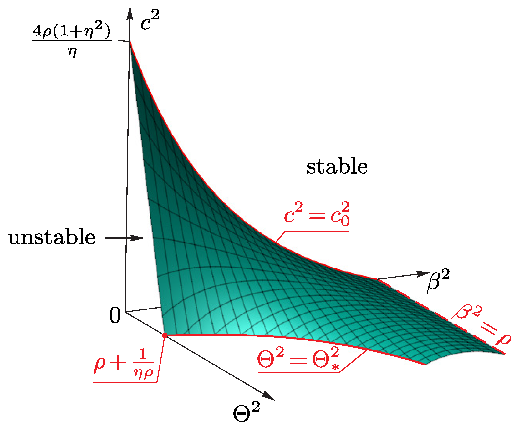
When , the surface depends on the parameters , , , and . The analysis of inequalities (37) and (38) implies that the regions of stability do not qualitatively change as the parameters , and are varied. Therefore, for ease of visualization we will depict the regions of stability in the parameter space for fixed values of the three remaining parameters.
Figure 5 shows the surface for the fixed values , and . If the parameter values lie below the surface, the vertical rotations are unstable, and if they lie above it, the vertical rotations are stable. It can be seen from the figure that, after the vibrations of the plane () are added, the vertical rotations become stable for smaller values of the angular momentum c.
4.3. Analysis of Reaction
In investigating the motion of rigid bodies on a plane, especially a moving one, special attention should be given to analysis of the normal reaction in order to avoid the loss of contact of the body with the plane during its motion. In the case at hand, the reaction of the plane, N, is expressed as follows:
where is the undetermined multiplier calculated in deriving the equations of motion. It is easy to verify that for the averaged system the normal reaction calculated for vertical rotations has the form
i.e., averaging smooths out the jumps of the normal reaction. Thus, within the framework of the averaged model, it is impossible to investigate the loss of contact of the body with the plane under vertical rotations which is due to vibrations of the plane.
For the exact system (8), in the case of vertical rotations, the normal reaction depends on time and has the form , and its minimal value for a period is
For the body to move without loss of contact with the plane, the condition must be satisfied. Since in the averaging procedure we assume that , the motion without loss of contact with the plane is only possible for sufficiently small amplitudes . In the averaged model, such amplitudes correspond to the small vibrational torque .
A more complete analysis of the possibility of stabilization without loss of contact with the plane should be made using a complete (unaveraged) model. Such an analysis of the reaction for a sphere with an internal pendulum rolling on a rough vibrating plane is carried out in [9].
5. Conclusions
In this paper, we have treated the problem of an axisymmetric ellipsoid rolling on a vertically vibrating plane. It was shown that, for an arbitrary convex body of revolution with axisymmetric mass distribution, the equations describing the dynamics of the system will preserve two integrals which are linear in angular momenta and, in the general case, are nonalgebraic functions of . Following [10], we have obtained an averaged time-independent vibrational potential which is invariant under rotation about the vertical axis. It is well known [37] that, in the presence of such a potential, the problem of a body of revolution rolling on a plane is integrable. Using the results of the above-mentioned paper, we have reduced the system under consideration to a system with one degree of freedom. As an example, we have constructed the phase portrait of the system.
To illustrate the influence of vibrations of the supporting plane on the ellipsoid’s dynamics, we have analyzed the stability of vertical rotations. The research results have shown that in the presence of a vibrational potential the vertical rotations of the ellipsoid become stable for smaller values of the angular velocity than those in the case of absence of vibrations. Moreover, there exists a critical value of a magnitude of the vibrational potential such that the vertical position can become stable even in the absence of rotation. In the limiting case of a thin rod, the resulting value of is the same as the value obtained by P. L. Kapitsa in [1].
To conclude, we point out the most interesting directions for the investigation of this problem. Further inquiry into the problem can involve the search for permanent rotations of the system and their bifurcation analysis. It would also be interesting to investigate the influence of a vibrational potential on the possibility of tumbling (similar to the tippe top inversion) of an ellipsoid with the center of mass displaced and friction forces added. A study of the tumbling of ellipsoidal bodies on a fixed plane was made in [21], where conditions on the system’s mass-geometric parameters for which a complete or partial inversion is possible were obtained.
Author Contributions
Conceptualization, A.A.K. and E.N.P.; investigation, A.A.K. and E.N.P.; writing—original draft preparation, E.N.P.; writing—review and editing, A.A.K. All authors have read and agreed to the published version of the manuscript.
Funding
The work of A.A.K. was performed at the Ural Mathematical Center (Agreement No 075-02-2023-933). The work of E.N.P. was carried out within the framework of the state assignment of the Ministry of Science and Higher Education of Russia (FEWS-2020-0009).
Data Availability Statement
Not applicable.
Acknowledgments
The authors thank I. S. Mamaev for fruitful discussions and valuable comments.
Conflicts of Interest
The authors declare no conflict of interest.
References
- Kapitza, P. A pendulum with oscillating suspension. Uspekhi Fiz. Nauk 1951, 44, 7–20. [Google Scholar] [CrossRef]
- Kapitza, P. Dynamic stability of a pendulum when its point of suspension vibrates. Sov. Phys. JETP 1951, 21, 588–597. [Google Scholar]
- Stephenson, A. On a new type of dynamical stability. Mem. Proc. Manch. Lit. Phil. Sci. 1908, 52, 1–10. [Google Scholar]
- Bardin, B.S.; Markeyev, A.P. The stability of the equilibrium of a pendulum for vertical oscillations of the point of suspension. J. Appl. Math. Mech. 1995, 59, 879–886. [Google Scholar] [CrossRef]
- Udwadia, F.E.; Di Massa, G. Sphere rolling on a moving surface: Application of the fundamental equation of constrained motion. Simul. Model. Pract. Theory 2011, 19, 1118–1138. [Google Scholar] [CrossRef]
- Awrejcewicz, J.; Kudra, G. Dynamics of a wobblestone lying on vibrating platform modified by magnetic interactions. Procedia IUTAM 2017, 22, 229–236. [Google Scholar] [CrossRef]
- Borisov, A.V.; Ivanov, A.P. Dynamics of the Tippe Top on a Vibrating Base. Regul. Chaotic Dyn. 2020, 25, 707–715. [Google Scholar] [CrossRef]
- Kilin, A.A.; Pivovarova, E.N. Nonintegrability of the problem of a spherical top rolling on a vibrating plane. Vestnik Udmurt. Univ. Mat. Mekhanika Komp Yuternye Nauk. 2020, 30, 628–644. [Google Scholar] [CrossRef]
- Kilin, A.A.; Pivovarova, E.N. Stability and stabilization of steady rotations of a spherical robot on a vibrating base. Regul. Chaotic Dyn. 2020, 25, 729–752. [Google Scholar] [CrossRef]
- Borisov, A.V.; Ivanov, A.P. A Top on a Vibrating Base: New Integrable Problem of Nonholonomic Mechanics. Regul. Chaotic Dyn. 2022, 27, 2–10. [Google Scholar] [CrossRef]
- Kilin, A.A.; Pivovarova, E.N. A Particular Integrable Case in the Nonautonomous Problem of a Chaplygin Sphere Rolling on a Vibrating Plane. Regul. Chaotic Dyn. 2021, 26, 775–786. [Google Scholar] [CrossRef]
- Kilin, A.A.; Pivovarova, E.N. Motion control of the spherical robot rolling on a vibrating plane. Appl. Math. Model. 2022, 109, 492–508. [Google Scholar] [CrossRef]
- Markeyev, A.P. The equations of the approximate theory of the motion of a rigid body with a vibrating suspension point. J. Appl. Math. Mech. 2011, 75, 132–139. [Google Scholar] [CrossRef]
- Ryabov, P.E.; Sokolov, S.V. Bifurcation Diagram of the Model of a Lagrange Top with a Vibrating Suspension Point. Mathematics 2023, 11, 533. [Google Scholar] [CrossRef]
- Karapetian, A. On stability of steady motions of a heavy solid body on an absolutely smooth horizontal plane. J. Appl. Math. Mech. 1981, 45, 368–373. [Google Scholar] [CrossRef]
- Karapetyan, A.; Rumyantsev, V. Stability of Conservative and Dissipative Systems. In Advances in Science and Technology. Series General Mechanics; Vsesoyuz. Inst. Nauch. Tekhn. Inform.: Moscow, Russia, 1983; Volume 6. [Google Scholar]
- Markeev, A.; Moshchuk, N. Qualitative analysis of motion of a heavy solid body on a smooth horizontal plane. J. Appl. Math. Mech. 1983, 47, 22–26. [Google Scholar] [CrossRef]
- Rumiantsev, V. Stability of rotation of a heavy gyrostat on a horizontal plane. Mech. Solids 1980, 15, 1–10. [Google Scholar]
- Karapetyan, A.; Rubanovskii, V. The bifurcation and stability of permanent rotations of a heavy triaxial ellipsoid on a smooth plane. J. Appl. Math. Mech. 1987, 51, 202–208. [Google Scholar] [CrossRef]
- Ivochkin, M.Y. Topological analysis of the motion of an ellipsoid on a smooth plane. Sb. Math. 2008, 199, 871. [Google Scholar] [CrossRef]
- Rauch-Wojciechowski, S.; Przybylska, M. On Dynamics of Jellet’s Egg. Asymptotic Solutions Revisited. Regul. Chaotic Dyn. 2020, 25, 40–58. [Google Scholar] [CrossRef]
- Bou-Rabee, N.M.; Marsden, J.E.; Romero, L.A. A geometric treatment of Jellett’s egg. ZAMM-J. Appl. Math. Mech. Angew. Math. Mech. Appl. Math. Mech. 2005, 85, 618–642. [Google Scholar] [CrossRef]
- Mindlin, I. The stability of the motion of a heavy solid of revolution on a horizontal plane. Inzh. Zh 1964, 4, 225–230. [Google Scholar]
- Mindlin, I.; Pozharitskii, G. On the stability of steady motions of a heavy body of revolution on an absolutely rough horizontal plane. J. Appl. Math. Mech. 1965, 29, 879–883. [Google Scholar] [CrossRef]
- Markeev, A. On the motion of a heavy homogeneous ellipsoid on a fixed horizontal plane. J. Appl. Math. Mech. 1982, 46, 438–449. [Google Scholar] [CrossRef]
- Markeev, A. The rolling of an ellipsoid on a horizontal plane. Mekhanika Tverd. Tela 1983, 18, 53–62. [Google Scholar]
- Karapetyan, A. Families of permanent rotations of triaxial ellipsoid on rough horizontal plane and their branchings. In Actual Problems of Classical and Celestial Mechanics; OOO “El’f” Ltd.: Moscow, Russia, 1998; pp. 46–51. [Google Scholar]
- Bizyaev, I.A.; Mamaev, I.S. Permanent Rotations in Nonholonomic Mechanics. Omnirotational Ellipsoid. Regul. Chaotic Dyn. 2022, 27, 587–612. [Google Scholar] [CrossRef]
- Tkhai, V. Instability of permanent rotations of a heavy homogeneous ellipsoid of revolution on an absolutely rough plane. Ross. Akad. Nauk Izv. Mekhanika Tverd. Tela 1992, 2, 25–30. [Google Scholar]
- Glukhikh, Y.; Tkhai, V.; Chevallier, D. On the Stability of Permanent Rotations of a Heavy Homogeneous Ellipsoid on the Rough Plane. In Problems of Studying the Stability and Stabilization of Motion; CC RAS: Moscow, Russia, 2000; pp. 87–104. [Google Scholar]
- Bolsinov, A.V.; Kilin, A.A.; Kazakov, A.O. Topological monodromy as an obstruction to Hamiltonization of nonholonomic systems: Pro or contra? J. Geom. Phys. 2015, 87, 61–75. [Google Scholar] [CrossRef]
- Poincaré, H. Sur le forme nouvelle des equations de la mecanique. C. R. Acad. Sci. Paris 1901, 132, 369–371. [Google Scholar]
- Borisov, A.V.; Mamaev, I.S. Rigid Body Dynamics. In De Gruyter Studies in Mathematical Physics; De Gruyter: Berlin, Germany, 2018; Volume 57. [Google Scholar]
- Neimark, J.I.; Fufaev, N.A. Dynamics of Nonholonomic Systems; American Mathematical Society: Providence, RI, USA, 2004; Volume 33. [Google Scholar]
- Bogolyubov, N.; Mitropolskiy, Y. Asymptotic Methods in the Theory of Nonlinear Oscillations; Nauka: Moscow, Russia, 1974. [Google Scholar]
- Chaplygin, S.A. On a motion of a heavy body of revolution on a horizontal plane. Regul. Chaotic Dyn. 2002, 7, 119–130. [Google Scholar] [CrossRef]
- Borisov, A.; Mamaev, I. The Rolling Motion of a Rigid Body on a Plane and a Sphere. Hierarchy of Dynamics. Regul. Chaotic Dyn. 2002, 7, 177–200. [Google Scholar] [CrossRef]
- Routh, E.J. The Advanced Part of a Treatise on the Dynamics of a System of Rigid Bodies; Macmillan and Co.: London, UK, 1892. [Google Scholar]
- Borisov, A.V.; Mamaev, I.S.; Kilin, A.A. Dynamics of rolling disk. Regul. Chaotic Dyn. 2003, 8, 201–212. [Google Scholar] [CrossRef]
- Markeev, A.P. The Dynamics of a Body Contacting a Rigid Surface; Nauka: Moscow, Russia, 1992; p. 336. [Google Scholar]
Figure 1.
(a) Diagram of an ellipsoid on a vibrating plane and (b) image of the ellipsoid on a plane in a meridian section.
Figure 1.
(a) Diagram of an ellipsoid on a vibrating plane and (b) image of the ellipsoid on a plane in a meridian section.
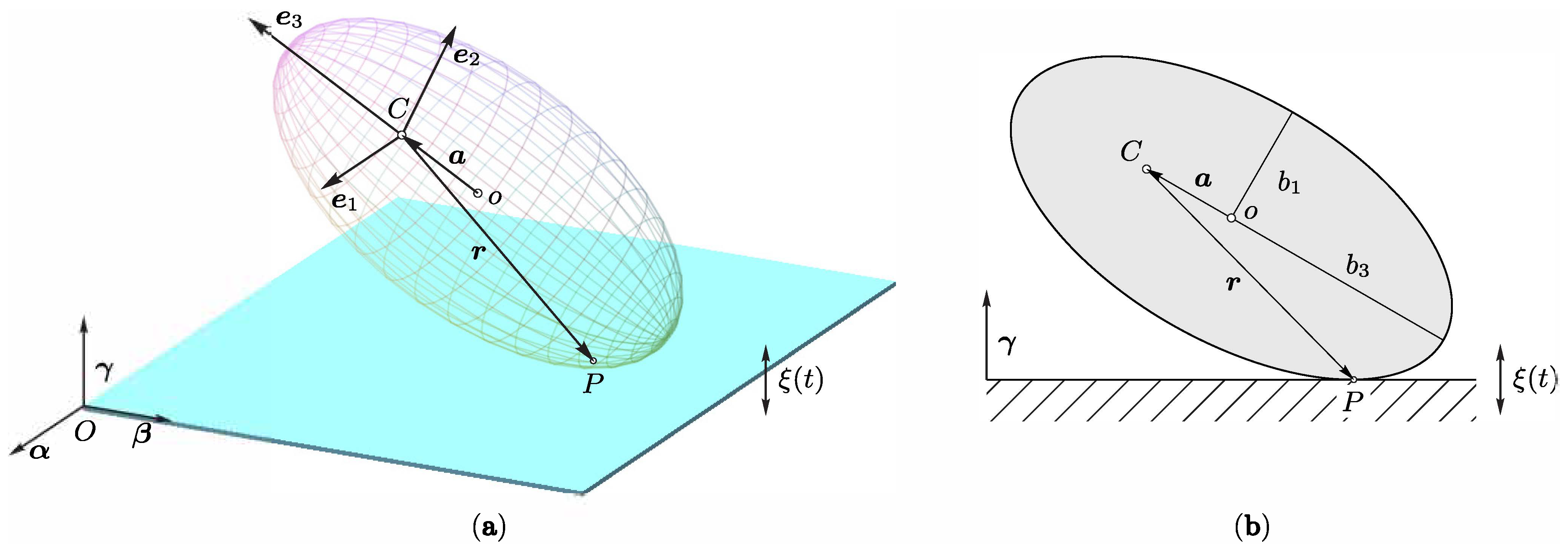
Figure 2.
An example of the phase portrait of the system (31), constructed for the parameters , , , , and the values of the integrals , .
Figure 2.
An example of the phase portrait of the system (31), constructed for the parameters , , , , and the values of the integrals , .

Figure 3.
Types of fixed points (33) depending on the values of the coefficients and of the characteristic Equation (34).
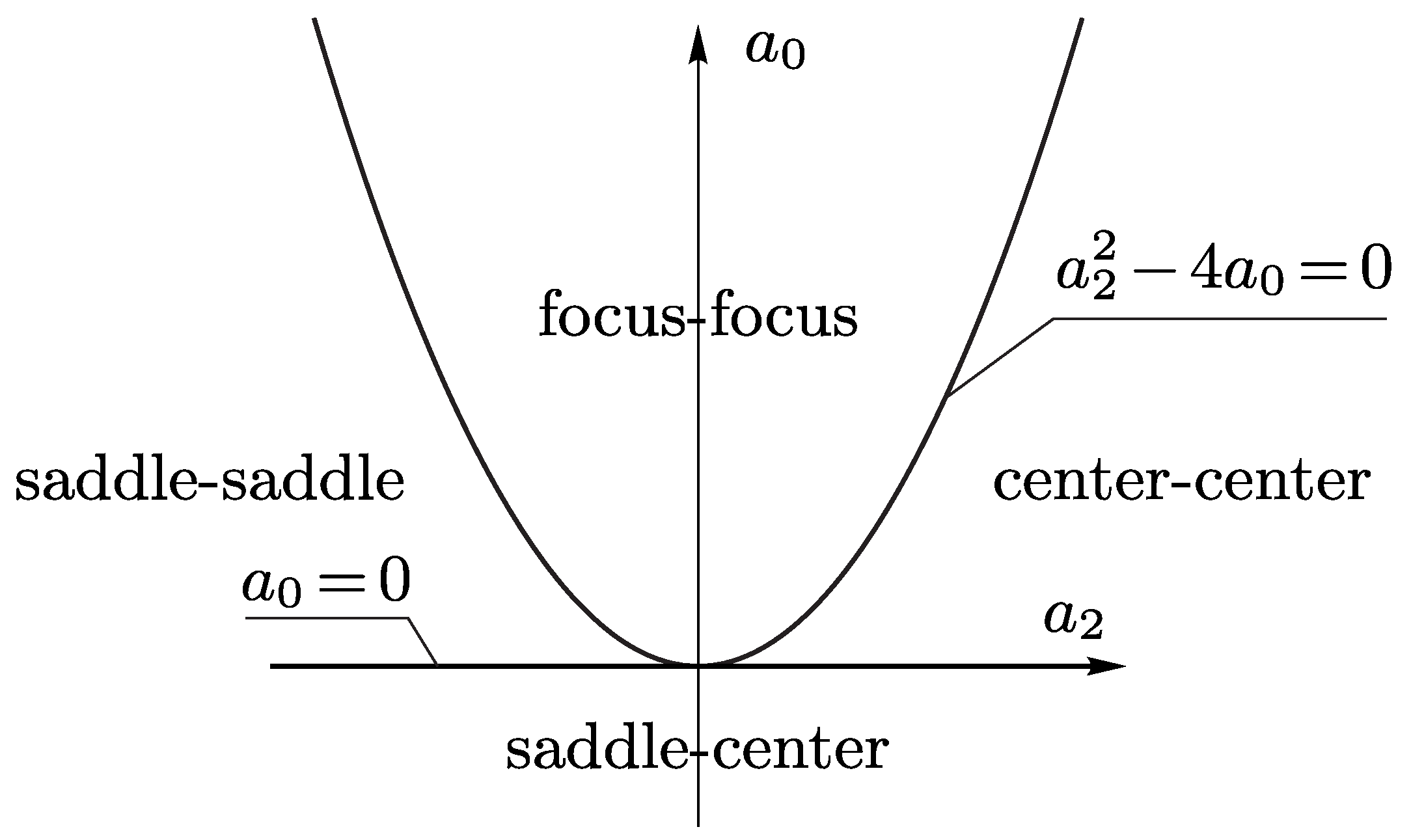
Figure 4.
The surface , which separates the regions of stable and unstable vertical rotations of the ellipsoid in the case of absence of a vibrational potential. The surface is plotted for and .
Figure 4.
The surface , which separates the regions of stable and unstable vertical rotations of the ellipsoid in the case of absence of a vibrational potential. The surface is plotted for and .

Figure 5.
The surface , which separates the regions of stable and unstable vertical rotations of the ellipsoid in the case of absence of a vibrational potential. The surface is plotted for , and .
Figure 5.
The surface , which separates the regions of stable and unstable vertical rotations of the ellipsoid in the case of absence of a vibrational potential. The surface is plotted for , and .
Disclaimer/Publisher’s Note: The statements, opinions and data contained in all publications are solely those of the individual author(s) and contributor(s) and not of MDPI and/or the editor(s). MDPI and/or the editor(s) disclaim responsibility for any injury to people or property resulting from any ideas, methods, instructions or products referred to in the content. |
© 2023 by the authors. Licensee MDPI, Basel, Switzerland. This article is an open access article distributed under the terms and conditions of the Creative Commons Attribution (CC BY) license (https://creativecommons.org/licenses/by/4.0/).
Share and Cite
MDPI and ACS Style
Kilin, A.A.; Pivovarova, E.N. Stability of Vertical Rotations of an Axisymmetric Ellipsoid on a Vibrating Plane. Mathematics 2023, 11, 3948. https://doi.org/10.3390/math11183948
AMA Style
Kilin AA, Pivovarova EN. Stability of Vertical Rotations of an Axisymmetric Ellipsoid on a Vibrating Plane. Mathematics. 2023; 11(18):3948. https://doi.org/10.3390/math11183948
Chicago/Turabian StyleKilin, Alexander A., and Elena N. Pivovarova. 2023. "Stability of Vertical Rotations of an Axisymmetric Ellipsoid on a Vibrating Plane" Mathematics 11, no. 18: 3948. https://doi.org/10.3390/math11183948
Note that from the first issue of 2016, this journal uses article numbers instead of page numbers. See further details here.