Abstract
In this paper, we define a new generator to propose continuous as well as discrete families (or classes) of distributions. This generator is used for the DAL model (acronym of the last names of the authors, Dimitrakopoulou, Adamidis, and Loukas). This newly proposed family may be called the new odd DAL (NODAL) G-class or alternate odd DAL G-class of distributions. We developed both a continuous as well as discrete version of this new odd DAL G-class. Some mathematical and statistical properties of these new G-classes are listed. The estimation of the parameters is discussed. Some structural properties of two special models of these classes are described. The introduced generators can be effectively applied to discuss and analyze the different forms of failure rates including decreasing, increasing, bathtub, and J-shaped, among others. Moreover, the two generators can be used to discuss asymmetric and symmetric data under different forms of kurtosis. A Monte Carlo simulation study is reported to assess the performance of the maximum likelihood estimators of these new models. Some real-life data sets (air conditioning, flood discharges, kidney cysts) are analyzed to show that these newly proposed models perform better as compared to well-established competitive models.
Keywords:
statistical model; odd G-class; discrete generators; failure analysis; dispersion phenomena; estimation; computer simulation; comparative study; statistics and numerical data MSC:
60E05; 62E10; 62E15; 62F10
1. Introduction
There is an increasing trend in modern distribution theory by which new flexible models are being tested in different fields through modifications, extended versions, and, most preferably, through generalized classes (G-classes). Suppose that is a mathematical function that helps in developing G-classes. In modern distribution theory, this function is described as a generator (i.e., a function which generates a G-class after fulfilling the desired criterion). Let T be a random variable (rv); then, the generator is basically a function of a baseline (or parent) cumulative distribution function (cdf) or survival function (sf) . and are the cdf and probability density function (pdf) of a new model or a G-class, and very few generators have been reported in the literature for developing new G-classes for an rv . In the literature the following probability classes/generators have been listed so far for any rv T:
- (i)
- for range ;
- (ii)
- , , (odds) and for range ;
- (iii)
- and (log-odds) for range .
The main objective of this article is to present a new G-class of distributions through some odds ratio (or function).
For a lifetime rv T, let be the basic odds function criterion, which naturally turns into ratio (reversed hazard rate function divided by the hazard rate function), as a useful measure for lifetime assessment of component(s) (or human organ(s)). Moreover, the probabilities of a uni-variate continuous rv spread over the range of the cdf and sf, that is, . So, the ratio between these two alternatives ( and ) is very useful in investigating changes occurring within a model or a phenomenon. Furthermore, these two alternatives are also the key elements for the order statistics, entropies, and records (upper and lower) density functions. The other odds function measures can be chosen as the ratio of the identities in upper and lower records (cumulative hazard rate function divided by the cumulative reversed hazard function), for instance:
- (i)
- Ratio of Lehmann alternatives , where is the power parameter (see Gupta et al. [1]);
- (ii)
- Log odds function (see Al-Aqtash et al. [2]);
- (iii)
- Logit function (see Torabi and Montazeri [3] and Zubair et al. [4]).
Based on the difference of the two log-odds functions, a well-established tool in survival analysis is the proportional odds model, say , where is the baseline log odds function and is the probability of failure by time t for an individual with .
Furthermore, Cooray [5] pioneered the concept of the odd function while dealing with probability models, and then he established the odd Weibull model. Gleaton and Lynch [6], while modeling the “strength distribution of an inhomogeneous bundle of brittle elastic fibers under equal load sharing and for checking implementation of the maximum entropy principal (MEP)”, proposed the generalized log-logistic transformation, which led to the odd log-logistic G-class. These two pioneering works motivated researchers and practitioners to develop odds-based G-classes, and to investigate special models from them. Some G-classes based on odd ratio , presented in the statistical literature, are included in Table 1. For more details about G-class, see Alzaatreh et al. [7].

Table 1.
Odd ratio for G-classes of distributions.
2. Background
Several authors have suggested modifications and enhancements to both the exponential and Weibull models in the recent past, with the aim of enhancing their empirical performance and increasing their flexibility. The most peculiar ones are the Lomax exponentiated Weibull model (Ansari and Nofal [34]), extended exponential (ExtE) or generalized exponential(GE) (see Gupta and Kundu [35]), and Nadarajah–Haghighi (NH) (see, Nadarajah and Haghighi [36]). The cdfs of the GE and NH models are
and
respectively, where is a scale parameter and is a power (or shape) parameter. Clearly, these two models reduce to the exponential model when .
Dimitrakopoulou, Adamidis, and Loukas [37] presented an extension of the Weibull model, in the so-called DAL. The cdf and its corresponding pdf of the DAL distribution can be formulated as
and
where the scale parameter is denoted by , while the shape (or power) parameters are indicated by and . For , the DAL model reduces to the Weibull, and for , the DAL distribution becomes the exponential model. Nowadays, the DAL model has also been reported as the power generalized Weibull (PGW) distribution (Nikulin and Haghighi [38,39]). However, there is some difference in parametrization of the DAL and PGW models, which is apparent from the cdf of the PGW model, as follows:
where is a scale parameter and and are shape (or power) parameters. Some generalizations/modifications of the DAL model were derived and discussed in the literature. See, for example, exponentiated-DAL (Peña-Ramírez et al. [40]), half-logistic-DAL (Anwar and Bibi [41]), DAL-Logarithmic (Tafakori et al. [42]), MO-DAL (Afify et al. [43]), and transmuted-DAL (Khan [44]).
In the literature, some odd-based G-classes have been discussed as extensions of the exponential or Weibull models, for instance, Bourguignon et al. [9], Tahir et al. [10], Nascimento et al. [28], El-Morshedy et al. [26], El-Morshedy and Eliwa [29], and Ahmad et al. [31] proposed the OW-G, odd generalized Weibull-G (OGW-G), OGE-G, ONH-G, OFW-H, OChen-G, and ODAL-G classes of distributions.
Recently, Hussain et al. [45] defined two new generators (i) and (ii) for bounded unit interval and then introduced two new Kumaraswamy G-classes of distributions from them. In this paper, we develop a new generator for , which seems less complicated in comparison to earlier published generators, but it performs better when compared with other models.
On the other hand, from the last two decades, discretizing continuous probability models has received wider attention in distribution theory. The phenomenon of discretization occurs when measuring the lifespan of a product or device becomes impractical or impossible on a continuous scale. In such cases, it may be necessary to record lifetimes on a discrete scale rather than a continuous one. This has led to the study of several discrete distributions in the literature. See, for example, Roy [46], Krishna and Pundir [47], Gómez-Déniz [48], Jazi et al. [49], Gómez-Déniz and Calderín-Ojeda [50], Hussain and Ahmad [51], Hussain et al. [52], Para and Jan [53,54], El-Morshedy et al. [55], Eliwa at al. [56], Eliwa and El-Morshedy [57], Eliwa et al. [58], among others. Despite the existence of several discrete probability models in the literature, there is still space for deriving new discretized probability distributions that are appropriate for various areas. To address this, our paper presents a flexible generator of discrete distributions, known as the discrete new odd DAL-G (DNODAL-G) family, which can cater to various conditions. Our proposal for introducing new G-classes is as follows:
- Generate probability models (ProM) with asymmetric “negatively-skewed, positively-skewed” or symmetric shapes;
- Define special ProM with all kinds of risk/failure rate functions;
- Propose ProM suitable for analyzing and discussing both over- and under-dispersed data;
- Develop ProM for modeling/analyzing both lifetime and counting data sets;
- Provide ProM that consistently produces a better fit than other ProM built using the same underlying model, in addition to other ProM known in the literature.
The article is organized as follows. A new odd G-class of distributions is introduced in Section 3. Some mathematical properties of a new G-class such as a linear representation for the density, moments, generating function, and estimation of the model parameters are addressed in Section 4. A new model (a special case of the newly proposed G-class for continuous rv) is studied in Section 5 along with a Monte Carlo simulation study. The new discrete odd G-class along with a sub-model is defined, and a Monte Carlo simulation study is investigated in Section 6. Empirical investigation of the proposed models is reported in Section 7 by means of real-life data sets. In Section 8, we conclude our paper with some remarks.
3. The New Odd DAL G-Class
Let T be an rv representing the lifetime of a stochastic system having a baseline distribution. If the rv X represents the odd ratio, then the risk that a system will not be working at time x is given by . Therefore, the randomness of X can be modelled by the cdf
where is the cdf of T, and then . The cdf of the odd DAL-G (NODALG) class is defined as
where is a scale parameter, and are shape parameters, and is the vector of the baseline parameters. The pdf corresponding to Equation (7) can be expressed as
Henceforth, the rv X with density (7) is denoted by . The hazard rate function (hrf) of X has the form
Here, we let , and to omit the dependence of the parameters.
Proposition.
Following [37], if , then the subsets of our proposed G-class are
- (i)
- If , then , for ;
- (ii)
- If , then ;
- (iii)
- If , then ;
- (iv)
- If , then ;
- (v)
- If , then ;
- (vi)
- If , then ;
- (vii)
- If , then ;
- (viii)
- If , then ;
- (ix)
- If , then ;
where Y is a random variable that can take different forms of probability generators.
4. Properties of the NKw-G Family
A G-class or a model is known from some important characteristics which they exhibit mathematically or graphically. In this segment, some mathematical and statistical features of the NKw-G class are derived, which will be useful for the readers.
4.1. Quantile Function
The quantile function (qf) is a useful statistical measure that is helpful in obtaining some useful properties, including simulation study. The qf of the NODAL-G class can be expressed as
where the u follows a uniform distribution over an interval , is the inverse function of base line cdf, and the Lambert-W function is the inverse function of . The power series expansion for using the software Mathematica 12 yields the principal solution for w in
where is used as Lambert-W function in the software Mathematica.
4.2. Linear Representation
Here, a useful expansion for Equation (8) is derived. By utilizing the exponential power series in Equation (7), we can write
For a real non-integer, the generalized binomial expansion holds , and then applying in Equation (9) gives
Using the previous expansion and the exponential power series, we obtain after some algebra
where
By differentiating Equation (10), the G-class density follows as
Equation (11) reveals that the NODAL-G family density is a linear combination of exponentiated-G (exp-G) densities. Then, some statistical properties of X can be obtained from Equation (11) and well-established properties of the exp-G distributions.
4.3. Moments
In this segment, the ordinary moment (om), lower incomplete moment (lincm), and moment generating function (mgf) are derived. Let be an rv having the exp-G family with power parameter . First, the sth om of X, say , can be expressed from Equation (11) as
where , and is qf of baseline G. The well-known relationships can be used to derive the central moments and cumulants of X from Equation (12). Second, the sth lincm of X, say , is
For most G distributions, it is possible to numerically evaluate the last two integrals in the equation. The first lincm, , is useful in constructing popular measures such as Bonferroni and Lorenz curves in various fields such as demography, economics, reliability, medicine, and insurance. In addition, it can also be applied to determine the sum of the deviations from the mean and median of X. Furthermore, the mgf of X can be derived from (11).
where is the mgf of and . Therefore, we can derive the mgfs of several particular NODAL-G models directly from Equation (14) and exp-G generating functions.
4.4. Maximum Likelihood Estimation
Uncensored maximum likelihood estimation, in which all of the data are observed without any censoring, is a technique for estimating the parameters of a probability distribution based on a sample of data. This segment deals with the estimation of the unknown NODAL-G class parameters via the maximum likelihood (ML) approach. The ML estimation refers to a method of estimating unknown parameters by selecting values that maximize the likelihood of observing a given set of data. This technique is often used in various types of statistical modeling, such as regression and classification. It is a popular approach due to its simplicity and the fact that it is easy to implement. At its core, ML estimation is a mathematical approach for finding the probability distribution of a unknown variable based on a given sample of data. This is achieved by finding the maximum value of the likelihood function, which is based on the probability distribution of the given data. The likelihood function is computed by taking the product of the probability of the observations in the data set. Max likelihood estimation is used in many areas of study, including economics, biology, engineering, and computer science. As an example, in economics, it is used to make predictions about the probability of future events based on past observations. In biology, it is used to estimate gene frequencies and relationships between genes. For more details about the ML approach and its statistical properties, see Casella and Berger [59]. The log-likelihood function for the parameter vector can be derived from n observations/notes .
One way to find the maximum likelihood estimate (MLE) of is to maximize the likelihood function . There are several numerical optimization routines available in different programming languages such as R, SAS, and Ox that can be used to maximize . For instance, the optim function in R, the PROC NLMIXED in SAS, and the (sub-routine MaxBFGS) Ox can be used for this purpose.
5. The NODAL-Weibull Distribution
In this Section, we consider a special model of the NODAL-G class, the NODAL-Weibull (NODALW) distribution, by taking the Weibull as a baseline model. The cdf and pdf of Weibull distributions are and , respectively, where is a scale parameter and is a shape parameter. By setting , the cdf of the NODALW distribution reduces to
The pdf corresponding to Equation (15) is
Henceforth, let be the rv with density (16). The hrf of X is
The sketches of the density and failure rate of X are plotted in Figure 1 for some parameter values. Figure 1a displays the uni-modal (right-skewed and left-skewed) and reversed-J shapes of the density of X. Figure 1b exhibits the failure rate shapes of X such as increasing, decreasing, and bathtub.
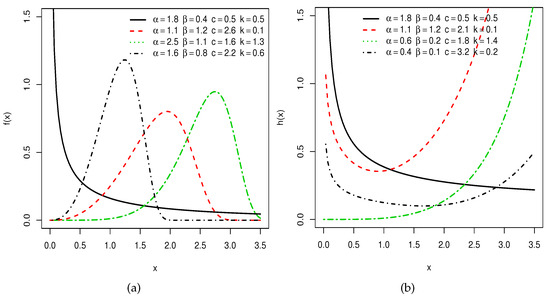
Figure 1.
Sketches of (a) the densities, and (b) the hrf of the NODALW model.
5.1. Linear Representation of NODALW Model
The NODALW density follows from Equation (11) as
Using the generalized binomial expansion in Equation (17), we obtain
where . Equation (18) reveals that the NODALW density has a linear representation in terms of Weibull densities. So, several of its structural properties can be obtained from the Weibull density. The qf of the NODALW distribution is
5.2. Properties of NODALW Model
Let be an rv with Weibull density . Then, some quantities of X can follow from those of . First, the sth om of X can be expressed as
where . Using Equation (20), we can recursively calculate the cumulants () of X. Specifically, the sth cumulant is determined by subtracting the sum of products of previous cumulants () and raw moments (), where the products are taken over all k from 1 to , inclusive. The formula is expressed as
The first cumulant, , is equal to the first raw moment, . The skewness, , and kurtosis, , of X can be obtained by dividing the third and fourth standardized cumulants by the square of the second standardized cumulant, respectively. Some plots of skewness (sk) and kurtosis (ku) for X are presented in Figure 2. It can be seen that the proposed class can be used to discuss the different forms of kurtosis.
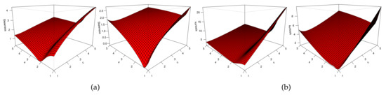
Figure 2.
Plots of the (a) sk and (b) ku of the NODALW model.
The sth incomplete moment of X, denoted by , is easily obtained by changing variables from the lower incomplete gamma function when calculating the corresponding moment of . Then, we obtain
5.3. Simulation Study: NODALW Model
Simulation studies are a popular and effective method of testing estimator performance in a variety of scenarios. By running several simulations, it is possible to approximate real-world performance and gain insight into how well the estimator will function in the field. The first step of a simulation study is to establish the parameters of the experiment. This involves setting up criteria for the data to be sampled, including number of samples, sample size, and the sampling process. Once the parameters have been established, the next step is to generate a simulated dataset that matches the specified criteria. This dataset should have features that are as close as possible to the features of the real-world data. Once the dataset has been generated, the estimator can be applied to the data. Depending on the type of estimator, different metrics may be used to measure the performance of the estimator. These metrics may include root mean squared error, mean absolute error, and R-squared. In this Section, we conduct a Monte Carlo simulation study to assess the performance of the MLEs of the parameters , , c, and k. The random numbers of size 50, 100, 200, and 500 are generated by the inversion method and are repeated times for each sample size. The sample average biases (Bias), coverage probabilities (CPs), and mean-squared errors (MSEs) of the estimates are calculated. The following formulas are used:
and
where is the indicator function and are the standard errors of the MLEs. These quantities for some values of , , c, and k are reported in Table 2, Table 3 and Table 4. The figures in these tables reveal that the MLEs perform well for estimating the parameters of the NODALW distribution.
Table 2.
Biases, MSEs, and CPs for , , , and .
Table 3.
Biases, MSEs, and CPs for , , , and .
Table 4.
Biases, MSEs, and CPs for , , , and .
6. Discrete NODAL-G Family
According to a survival discretization approach, the rv X is said to have the discrete NODAL-G (dNODAL-G) class if its cdf can be formulated as
where is a scale parameter, and are shape parameters, is the vector of the baseline parameters, and . The probability mass function (pmf) and hrf corresponding to Equation (22) are
and , respectively, where .
6.1. The DNODAL-Geometric (DNODALGeo) Distribution
Consider the cdf of the geometric (Geo) model. Then, the pmf of the DNODALGeo distribution is
where , and . For convenience, let in Equation (24). Figure 3 and Figure 4 display the pmf and hrf of the DNODALGeo distribution for some parameter values.
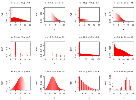
Figure 3.
The pmf of the DNODALGeo model.
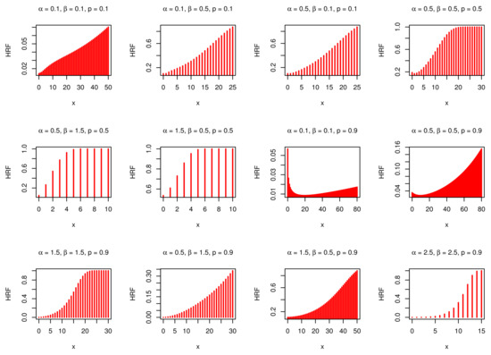
Figure 4.
The hrf of the DNODALGeo model.
PMF can be either monomodal or bimodal and can be used to analyze different types of data (positively skewed, negatively skewed, as well as symmetric). Moreover, hrf can be either an increment, a fixed increment, a J-shape, or a bathtub.
6.2. Simulation
We generate a random variable X from the DNODALGeo distribution by generating the value Z from the continuous model and then discretize , which is the largest integer less than or equal to Z. We generate samples of size from the DNODALGeo and DNODALGeo models, respectively. The empirical results are given in Figure 5 and Figure 6, respectively.
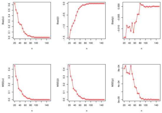
Figure 5.
The biases and MSEs for the DNODALGeo(0.5, 0.9, 0.8) model.
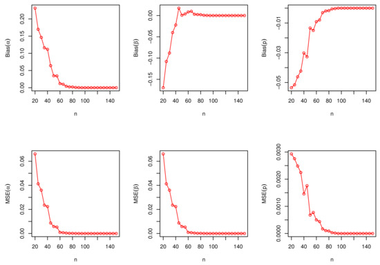
Figure 6.
The biases and MSEs for the DNODALGeo(1.5, 1.5, 0.5) model.
7. Applications
In this Section, we illustrate the empirical importance of the NODALW and DNODALGeo models by means of three real-life data sets. First, two data sets are utilized to illustrate the flexibility of the NODALW distribution. Second, a third data set is used to test the usefulness of the DNODALGeo distribution.
7.1. Empirical Illustration of the NODAL-G Family
Here, we compare the NODALW distribution with some well-established competitive models: Kumaraswamy–Weibull (KwW) (see Cordeiro et al. [60]), beta-Weibull (BW) (see Lee et al. [61]), exponentiated-generalized Weibull (EGW) (see Oguntunde et al. [62]), McDonald-Weibull (McW) (see Cordeiro et al. [63]), gamma-Weibull (GaW) (see Cordeiro et al. [64]), and Weibull (W) to prove the flexibility of the new family. The cdf and pdf of NODALW distribution are, respectively, given as
and
- Data Set 1. Air Conditioning Data. The data are taken from Kus [65] representing the numbers of the successive failures for an air conditioning system. The shape of the data can be discussed through Figure 7. The data were found to be asymmetric and some extreme observations were reported.
- Data Set 2. Precipitation Data. The data are taken from Katz et al. [66] and Asgharzadeh et al. [67] representing the maximum annual flood discharges (in units of 1000 cubic feet per second) of the North Saskachevan River at Edmonton, over a period of 48 years. The shape of the data can be displayed in Figure 8.
The NODALW model and other competitive models are fitted to these two data sets using the AdequacyModel package for the R statistical computing environment written by Marinho et al. [68].
The MLEs () are used to evaluate the log-likelihood function, while various goodness-of-fit statistics (“GoFS”), such as Akaike-information-criterion (“AIC”), Bayesian-information-criterion (“BIC”), Hannan-Quinn-information criterion (“HQIC”), Anderson–Darling (AD), Cramér–von Mises (CvM), and Kolmogrov–Smirnov (KS), are employed to compare models. A good fit is indicated by lower values of these statistics and higher P-values of the KS statistic.
The values of the GoFS in Table 5 and Table 7 show that the NODALW model gives small values for these statistics and then it provides the best fit as compared to other fitted distributions (KwW, BW, EGW, McW, GaW, and W) to the two data sets. Table 6 and Table 8 report the MLEs and their standard errors (SEs) for the NODALW model and other competitive models. The plots in Figure 9 and Figure 10 also support our claim. To establish the unique property of the maximum likelihood estimators, the profile log-maximum likelihood function (pllf) was plotted for each parameter for the first and second datasets. It can be noted that the values of the estimators gave the maximum likelihood function the largest value; see Figure 11 and Figure 12. As can be seen, the form of the maximum likelihood function is unimodal for each parameter.
Table 5.
Some statistics and p-value for the fitted models to data set 1.
Table 7.
Some statistics and p-value for the fitted models to data set 2.
Table 6.
MLEs and their SEs (in parentheses) for the fitted models to data set 1.
Table 8.
MLEs and their SEs (in parentheses) for the fitted models to data set 2.

Figure 7.
Non-parametric visualization plots for data set I.

Figure 8.
Non-parametric visualization plots for data set II.

Figure 9.
Plots of estimated density, cdf, Kaplan–Meier (K-M), and hrf plots for data set 1.

Figure 10.
Plots of estimated density, cdf, Kaplan–Meier (K-M), and hrf plots for data set 2.

Figure 11.
The pllf of data set 1.

Figure 12.
The pllf of data set 2.
7.2. Empirical Illustration of the DNODAL-G Family
Here, we illustrate the usefulness of the DNODALGeo model by means of an application to real count data. The data set represents the count of kidney cysts using steroids (see Chan et al. [69]). The shape of the data can be seen in Figure 13. The fitted distributions are compared using the AIC, CAIC, HQIC, and Chi-square (), having a degree of freedom (df) and its p-value. The competitive fitted models are reported in Table 9.
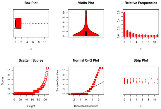
Figure 13.
Non-parametric visualization plots for data set III.
Table 9.
The competitive models.
The MLEs and their corresponding SEs are listed in Table 10, whereas Table 11 and Table 12 give the GoFS, expected frequencies (ExFr), and observed frequencies (ObFr), respectively.
Table 10.
The MLEs and their SEs for data set 3.
Table 11.
The GoFS for data set 3 “part I”.
Table 12.
The GoFS for data set 3 “part II”.
The DNODALGeo model performs better than all other tested models based on the numbers in Table 11 and Table 12. Figure 14 supports the claims from these tables, and it is noted that data set 3 is explained by this model. Figure 15 shows the contour plot of log-Likelihood function of the DNODALGeo for the third data set.
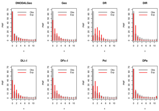
Figure 14.
The fitted PMFs to data set 3.
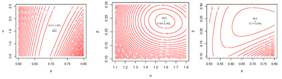
Figure 15.
Contour plot of pllf for data set 3.
8. Concluding Remarks and Future Work
In this article, a new odd DAL-G family of models is presented from a new class/generator for . The new probability family involves a different function of the cdf instead of existing generators. We obtain some structural properties of this new continuous and discussed discrete odd DAL-G family, and also studied some properties of the special models called the new odd DAL-Weibull (NODALW) and discrete new odd DAL-geometric (DNODALGeo) distributions. Both of two sub-models can be used to discuss asymmetric and symmetric data under different kinds of kurtosis. Furthermore, the two sub-models can be applied to discuss several shapes of risk/hazard rates. We compared the NODALW distribution with the well-known extended Weibull models (KwW, BW, EGW, McW, GaW, W) via six popular test statistics. Similarly, we compare the DNODALGeo distribution with the well-known extended models’ (Geo, GGeo, DR, DIR, DIW, DLi-I, DLi-II, DLi-III, NeBi, Poi, DPa, DB-XII, DLogL, DFx-I, DLo) distributions using these test statistics. We found that the new generated distributions provide better estimates and minimum values of the test statistics. The new NODALW and DNODALGeo models outperform the above-described competitive models on the basis of numerical and graphical analysis. We foresee that the new family/class will be able to attract readers and applied statisticians. As a future work, the bivariate extension of the proposed generators with its applications will be discussed. Furthermore, some prediction models will be analyzed based on these generators.
Author Contributions
Conceptualization, M.S.E. and M.A.H.; Methodology, M.E.-M.; Software, M.A.H., B.A. and M.E.-M.; Validation, M.A.H. and M.E.-M.; Formal analysis, M.S.E., M.H.T. and A.A.-B.; Resources, B.A and M.E.-M.; Data curation, M.S.E., B.A. and A.A.-B.; Writing—original draft, M.H.T., M.S.E. and M.A.H.; Writing—review & editing, M.S.E., M.A.H. and A.A.-B.; Visualization, B.A. and M.E.-M.; Supervision, M.H.T. All authors have read and agreed to the published version of the manuscript.
Funding
The paper did not receive any fund.
Data Availability Statement
The data sets are available in the paper.
Acknowledgments
The researchers would like to thank the Deanship of Scientific Research, Qassim University for funding publication of this project.
Conflicts of Interest
The authors declare no conflict of interests.
References
- Gupta, R.C.; Gupta, P.L.; Gupta, R.D. Modeling failure time data by Lehman alternatives. Commun. Stat. Theory Methods 1998, 27, 887–904. [Google Scholar] [CrossRef]
- Al-Aqtash, R.; Lee, C.; Famoye, F. Gumbel-Weibull distribution: Properties and applications. J. Mod. Appl. Stat. Methods 2014, 13, 201–225. [Google Scholar] [CrossRef]
- Torabi, H.; Montazeri, N.H. The logistic-uniform distribution and its application. Commun. Stat. Simul. Comput. 2014, 43, 2551–2569. [Google Scholar] [CrossRef]
- Zubair, M.; Pogany, T.K.; Cordeiro, G.M.; Tahir, M.H. The log-odd normal generalized family of distributions with application. An. Acad. Bras. Ciênc. 2019, 91, e20180207. [Google Scholar] [CrossRef] [PubMed]
- Cooray, K. Generalization of the Weibull distribution: The odd Weibull family. Stat. Methodol. 2006, 6, 265–277. [Google Scholar] [CrossRef]
- Gleaton, J.U.; Lynch, J.D. Properties of generalized log-logistic families of lifetime distributions. J. Probab. Stat. Sci. 2006, 4, 51–64. [Google Scholar]
- Alzaatreh, A.; Famoye, F.; Lee, C. A new method for generating families of continuous distributions. Metron 2013, 71, 63–79. [Google Scholar] [CrossRef]
- Torabi, H.; Montazeri, N.H. The gamma-uniform distribution and its application. Kybernetika 2012, 48, 16–30. [Google Scholar]
- Bourguignon, M.; Silva, R.B.; Cordeiro, G.M. The Weibull-G family of probability distributions. J. Data Sci. 2014, 12, 53–68. [Google Scholar] [CrossRef]
- Tahir, M.H.; Cordeiro, G.M.; Alizadeh, M.; Mansoor, M.; Zubair, M.; Hamedani, G.G. The odd generalized exponential family of distributions with applications. J. Stat. Distrib. Appl. 2015, 2, 1. [Google Scholar] [CrossRef]
- Hassan, A.S.; Hemeda, S.E. A new family of additive Weibull-generated distributions. Int. J. Math. Appl. 2016, 4, 151–164. [Google Scholar]
- Gomes-Silva, F.S.; Percontini, A.; de Brito, E.; Ramos, M.W.; Venancio, R.; Cordeiro, G.M. The odd Lindley-G family of distribution. Austrian J. Stat. 2017, 46, 65–87. [Google Scholar] [CrossRef]
- Cordeiro, G.M.; Alizadeh, M.; Ramires, T.G.; Ortega, E.M.M. The generalized odd half-Cauchy family of distributions: Properties and applications. Commun. Stat. Theory Methods 2017, 46, 5685–5705. [Google Scholar] [CrossRef]
- Afify, A.Z.; Altun, E.; Alizadeh, M.; Ozel, G.; Hamedani, G.G. The odd exponentiated half-logistic-G Family: Properties, characterizations and applications. Chil. J. Stat. 2017, 8, 65–91. [Google Scholar]
- Jamal, F.; Nasir, M.A.; Tahir, M.H.; Montazeri, N.H. The odd Burr-III family of distributions. J. Stat. Appl. Probab. 2017, 6, 105–122. [Google Scholar] [CrossRef]
- Yousof, H.M.; Afify, A.Z.; Hamedani, G.G. The Burr X generator of distributions for lifetime data. J. Stat. Theory Appl. 2017, 16, 288–305. [Google Scholar] [CrossRef]
- Cordeiro, G.M.; Yousof, H.M.; Ramires, T.G.; Ortega, E.M.M. The Burr XII system of densities: Properties, regression model and applications. J. Stat. Comput. Simul. 2018, 88, 432–456. [Google Scholar] [CrossRef]
- Haq, M.A.U.; Elgarhy, M. The odd Fréchet-G family of probability distributions. J. Stat. Appl. Probab. 2018, 7, 189–203. [Google Scholar] [CrossRef]
- Hassan, A.S.; Nassr, S.G. The inverse Weibull generator of distributions: Properties and applications. J. Data Sci. 2018, 16, 723–742. [Google Scholar] [CrossRef]
- Alizadeh, M.; Altun, E.; Cordeiro, G.M.; Rasekhi, M. The odd power-Cauchy family of distributions: Properties, regression models and applications. J. Stat. Comput. Simul. 2018, 88, 785–807. [Google Scholar] [CrossRef]
- Maiti, S.S.; Pramanik, S. A generalized Xgamma generator family of distributions. arXiv 2018, arXiv:1805.03892. [Google Scholar]
- Hassan, A.S.; Nassr, S.G. Power Lindley-G family of distributions. Ann. Data Sci. 2019, 6, 189–210. [Google Scholar] [CrossRef]
- Korkmaz, M.C.; Altun, E.; Yousof, H.M.; Hamedani, G.G. The odd power Lindley generator of probability distributions: Properties, characterizations and regression modeling. Int. J. Stat. Probab. 2019, 8, 70–89. [Google Scholar] [CrossRef]
- Cordeiro, G.M.; Afify, A.Z.; Ortega, E.M.M.; Suzuki, A.K.; Mead, M.E. The odd Lomax generator of distributions: Properties, estimation and applications. J. Comput. Appl. Math. 2019, 347, 222–237. [Google Scholar] [CrossRef]
- Kharazmi, O.; Saadatinik, A.; Alizadeh, M.; Hamedani, G.G. Odd hyperbolic cosine-FG family of lifetime distributions. J. Stat. Theory Appl. 2019, 18, 387–401. [Google Scholar] [CrossRef]
- El-Morshedy, M.; Eliwa, M.S. The odd flexible Weibull-H family of distributions: Properties and estimation with applications to complete and upper record data. Filomat 2019, 33, 2635–2652. [Google Scholar] [CrossRef]
- Aldahlan, M.A.; Afify, A.Z.; Ahmed, A.-H.N. The odd inverse Pareto-G class: Properties and applications. J. Nonlinear Sci. Appl. 2019, 12, 278–290. [Google Scholar] [CrossRef]
- Nascimento, D.C.; Silva, K.F.; Cordeiro, G.M.; Alizadeh, M.; Yousof, H.M.; Hamedani, G.G. The odd Nadarajah-Haghighi family of distributions: Properties and applications. Stud. Sci. Math. Hung. 2019, 56, 185–210. [Google Scholar] [CrossRef]
- El-Morshedy, M.; Eliwa, M.S.; Afify, A.Z. The odd Chen generator of distributions: Properties and estimation methods with applications in medicine and engineering. J. Natl. Sci. Found. Sri Lanka 2020, 48, 113–130. [Google Scholar]
- Anzagra, L.; Sarpong, S.; Nasiru, S. Odd Chen-G family of distributions. Ann. Data Sci. 2020, 9, 369–391. [Google Scholar] [CrossRef]
- Ahmad, Z.; Elgarhy, M.; Hamedani, G.G.; Butt, N.S. Odd generalized N-H generated family of distributions with application to exponential model. Pak. J. Stat. Oper. Res. 2020, 16, 53–71. [Google Scholar] [CrossRef]
- Nasir, M.A.; Tahir, M.H.; Chesneau, C.; Jamal, F.; Shah, M.A.A. The odds generalized gamma-G family of distributions: Properties, regression and applications. Statistica 2020, 80, 3–38. [Google Scholar] [CrossRef]
- Ishaq, A.I.; Abiodun, A.A. The Maxwell-Weibull distribution in modeling lifetime data sets. Ann. Data Sci. 2020, 7, 639–662. [Google Scholar] [CrossRef]
- Ansari, S.I.; Nofal, Z.M. The Lomax exponentiated Weibull model. Jpn. J. Stat. Data Sci. 2021, 4, 21–39. [Google Scholar] [CrossRef]
- Gupta, R.D.; Kundu, D. Generalized exponential distributions. Aust. N. Z. J. Stat. 1999, 41, 173–188. [Google Scholar] [CrossRef]
- Nadarajah, S.; Haghighi, F. An extension of the exponential distribution. Statistics 2011, 45, 54–558. [Google Scholar] [CrossRef]
- Dimitrakopoulou, T.; Adamidis, K.; Loukas, S. A lifetime distribution with an upside–down bathtub-shaped hazard function. IEEE Trans. Reliab. 2007, 56, 308–311. [Google Scholar] [CrossRef]
- Nikulin, M.; Haghighi, F. A chi-squared test for the generalized power Weibull family for the head-and-neck cancer censored data. J. Math. Sci. 2006, 133, 1333–1341. [Google Scholar] [CrossRef]
- Nikulin, M.; Haghighi, F. On the power generalized Weibull family: Model for cancer censored data. Metron 2009, 67, 75–86. [Google Scholar]
- Peńa-Ramírez, F.A.; Guerra, R.R.; Cordeiro, G.M.; Rinho, P.R.D. The exponentiated power generalized Weibull: Properties and applications. An. Acad. Bras. Ciêc. 2018, 90, 2553–2577. [Google Scholar] [CrossRef]
- Anwar, M.; Bibi, A. The half-logistic generalized Weibull distribution. J. Probab. Stat. 2018, 12, 8767826. [Google Scholar] [CrossRef]
- Tafakori, L.; Pourkhanali, A.; Nadarajah, S. A new lifetime model with different types of failure rate. Commun. Stat. Theory Methods 2018, 47, 4006–4020. [Google Scholar] [CrossRef]
- Afify, A.Z.; Kumar, D.; Elbatal, I. Marshall-Olkin power generalized Weibull distribution with applications in engineering and medicine. J. Stat. Theory Appl. 2020, 19, 223–237. [Google Scholar] [CrossRef]
- Khan, M.S. Transmuted generalized power Weibull distribution. Thail. Stat. 2018, 16, 156–172. [Google Scholar]
- Hussain, M.A. Some New Generalized Kumaraswamy Families of Distributions. Ph.D. Thesis, The Islamia University of Bahawalpur, Bahawalpur, Pakistan, 2020. [Google Scholar]
- Roy, D. Discrete Rayleigh distribution. IEEE Trans. Reliab. 2004, 53, 255–260. [Google Scholar] [CrossRef]
- Krishna, H.; Pundir, P.S. Discrete Burr and discrete Pareto distributions. Stat. Methodol. 2009, 6, 177–188. [Google Scholar] [CrossRef]
- Gómez-Déniz, E. Another generalization of the geometric distribution. Test 2010, 19, 399–415. [Google Scholar] [CrossRef]
- Jazi, M.A.; Lai, C.D.; Alamatsaz, M.H. A discrete inverse Weibull distribution and estimation of its parameters. Stat. Methodol. 2010, 7, 121–132. [Google Scholar] [CrossRef]
- Gómez-Déniz, E.; Calderín-Ojeda, E. The discrete Lindley distribution: Properties and applications. J. Stat. Comput. Simul. 2011, 81, 1405–1416. [Google Scholar] [CrossRef]
- Hussain, T.; Ahmad, M. Discrete inverse Rayleigh distribution. Pak. J. Stat. 2014, 30, 203–222. [Google Scholar]
- Hussain, T.; Aslam, M.; Ahmad, M. A two-parameter discrete Lindley distribution. Rev. Colomb. Estad. 2016, 39, 45–61. [Google Scholar] [CrossRef]
- Para, B.A.; Jan, T.R. Discrete version of log-logistic distribution and its applications in genetics. International J. Mod. Math. Sci. 2016, 14, 407–422. [Google Scholar]
- Para, B.A.; Jan, T.R. On discrete three parameter Burr type XII and discrete Lomax distributions and their applications to model count data from medical science. Biom. Biostat. Int. J. 2016, 4, 1–15. [Google Scholar]
- El-Morshedy, M.; Eliwa, M.S.; Altun, E. Discrete Burr-Hatke distribution with properties, estimation methods and regression model. IEEE Access 2020, 8, 74359–74370. [Google Scholar] [CrossRef]
- Eliwa, M.S.; Altun, E.; El-Dawoody, M.; El-Morshedy, M. A new three-parameter discrete distribution with associated INAR (1) process and applications. IEEE 2020, 8, 91150–91162. [Google Scholar]
- Eliwa, M.S.; El-Morshedy, M. A one-parameter discrete distribution for over-dispersed data: Statistical and reliability properties with estimation approaches and applications. J. Appl. Stat. 2022, 49, 2467–2487. [Google Scholar] [CrossRef] [PubMed]
- Eliwa, M.S.; Alhussain, Z.A.; El-Morshedy, M. Discrete Gompertz-G family of distributions for over-and under-dispersed data with properties, estimation, and applications. Mathematics 2020, 8, 358. [Google Scholar] [CrossRef]
- Casella, G.; Berger, R.L. Statistical Inference; Cengage Learning: Boston, MA, USA, 2021. [Google Scholar]
- Cordeiro, G.M.; Ortega, E.M.M.; Nadarajah, S. The Kumaraswamy Weibull distribution with application to failure data. J. Frankl. Inst. 2010, 347, 1399–1429. [Google Scholar] [CrossRef]
- Lee, C.; Famoye, F.; Olumolade, O. Beta-Weibull distribution: Some properties and applications to censored data. J. Mod. Appl. Stat. Methods 2007, 6, 173–186. [Google Scholar] [CrossRef]
- Oguntunde, P.E.; Odetunmibi, O.A.; Adejum, A.O. On the exponentiated generalized Weibull distribution: A generalization of the Weibull distribution. Indian J. Sci. Technol. 2015, 8, 1–7. [Google Scholar] [CrossRef]
- Cordeiro, G.M.; Hashimoto, E.M.; Ortega, E.M.M. The McDonald Weibull model. Statistics 2012, 48, 256–278. [Google Scholar] [CrossRef]
- Cordeiro, G.M.; Aristizábal, W.D.; Suárez, D.M.; Lozano, S. The gamma modified Weibull distribution. Chil. J. Stat. 2011, 6, 37–48. [Google Scholar]
- Kus, C. A new lifetime distribution. Comput. Stat. Data Anal. 2007, 51, 4497–4509. [Google Scholar] [CrossRef]
- Katz, R.W.; Parlange, M.B.; Naveau, P. Statistics of extremes in hydrology. Adv. Water Resour. 2002, 25, 1287–1304. [Google Scholar] [CrossRef]
- Asgharzadeh, A.; Bakouch, H.S.; Habibi, M. A generalized binomial exponential 2 distribution: Modeling and applications to hydrologic events. J. Appl. Stat. 2017, 44, 2368–2387. [Google Scholar] [CrossRef]
- Marinho, P.R.D.; Bourguignon, M.; Dias, C.R.B. Adequacy Model 1.0.8: Adequacy of Probabilistic Models and Generation of Pseudo-Random Numbers. 2015. Available online: http://cran.rproject.org/web/packages/AdequacyModel/AdequacyModel.pdf (accessed on 12 November 2015).
- Chan, S.K.; Riley, P.R.; Price, K.L.; McEldu, F.; Winyard, P.J.; Welham, S.J.; Woolf, A.S.; Long, D.A. Corticosteroid-induced kidney dysmorphogenesis is associated with deregulated expression of known cystogenic molecules, as well as Indian hedgehog. Am. J. Physiol.-Ren. Physiol. 2010, 298, F346–F356. [Google Scholar] [CrossRef]
- Poisson, S.D. Probabilité des Jugements en Matié re Criminelle et en Matiére Civile, Précédées des Régles Génerales du Calcul des Probabilitiés; Bachelier: Paris, France, 1837; pp. 206–207. [Google Scholar]
Disclaimer/Publisher’s Note: The statements, opinions and data contained in all publications are solely those of the individual author(s) and contributor(s) and not of MDPI and/or the editor(s). MDPI and/or the editor(s) disclaim responsibility for any injury to people or property resulting from any ideas, methods, instructions or products referred to in the content. |
© 2023 by the authors. Licensee MDPI, Basel, Switzerland. This article is an open access article distributed under the terms and conditions of the Creative Commons Attribution (CC BY) license (https://creativecommons.org/licenses/by/4.0/).