

Mathematical Analysis of Mixed Convective Peristaltic Flow for Chemically Reactive Casson Nanofluid

1
Department of Basic Sciences, Preparatory Year Deanship, King Faisal University, Al-Ahsa 31982, Saudi Arabia
2
Department of Computer Science, National University of Sciences and Technology (NUST), Balochistan Campus (NBC), Quetta 87300, Pakistan
*
Authors to whom correspondence should be addressed.
Mathematics 2023, 11(12), 2673; https://doi.org/10.3390/math11122673
Submission received: 17 May 2023
/
Revised: 9 June 2023
/
Accepted: 9 June 2023
/
Published: 12 June 2023
(This article belongs to the Special Issue Theoretical Research and Computational Applications in Fluid Dynamics)
Abstract
:Nanofluids are extremely beneficial to scientists because of their excellent heat transfer rates, which have numerous medical and industrial applications. The current study deals with the peristaltic flow of nanofluid (i.e., Casson nanofluid) in a symmetric elastic/compliant channel. Buongiorno’s framework of nanofluids was utilized to create the equations for flow and thermal/mass transfer along with the features of Brownian motion and thermophoresis. Slip conditions were applied to the compliant channel walls. The thermal field incorporated the attributes of viscous dissipation, ohmic heating, and thermal radiation. First-order chemical-reaction impacts were inserted in the mass transport. The influences of the Hall current and mixed convection were also presented within the momentum equations. Lubricant approximations were exploited to make the system of equations more simplified for the proposed framework. The solution of a nonlinear system of ODEs was accomplished via a numerical method. The influence of pertinent variables was examined by constructing graphs of fluid velocity, temperature profile, and rate of heat transfer. The concentration field was scrutinized via table. The velocity of the fluid declined with the increment of the Hartman number. The effects of thermal radiation and thermal Grashof number on temperature showed opposite behavior. Heat transfer rate was improved by raising the Casson fluid parameter and the Brownian motion parameter.
Keywords:
peristalsis; Casson fluid model; nanofluid; mixed convection; compliant walls; chemical reactionMSC:
35Q30; 35Q35; 76D051. Introduction
Heat transfer research is extremely useful in a wide range of engineering disciplines, such as evaporative cooling thrust bearing, drag reduction, and circular heat exchanger prototypes. Fluids are frequently used as thermal carriers in applications such as automotive cooling and heating and are a central role in the industrial process. Heat transfer enhancement can enhance the effectiveness of a thermoelectric generator. Heat transfer improvement can result in more compact cooling equipment, conserving fuel, space, and wealth. Comparing nanofluids to their base fluids reveals that they are more effective at transmitting heat and have better thermal conductivity. Consequently, it is widely acknowledged and appreciated from both a philosophical and empirical standpoint that distributing nanoparticles in a biofluid may enhance its thermophysical qualities. Nanofluids reduce energy use, improve thermal efficiency, speed up operations, and lengthen the useful life of the equipment. It was Choi [1] who initially suggested using nanofluids. Once these fluids were accepted by the scientific world, they immediately assumed a key function. Chon et al. [2] securitized how temperature and particle size are significant for enhancing the thermal conductivity of the Al2O3 nanomaterial. Thermophoresis and random motion spreading were named by Buongiorno [3] as the most crucial factors in enhancing common liquids’ capacity to transmit heat. Tripathi and Bég [4] elaborated on the peristalsis of nanofluid in a drug delivery system in biomedical science. The peristaltic motion of a nanoliquid with wall and slip characteristics was explored by Hayat et al. [5]. The hydrothermal characteristics of magnetohydrodynamic (MHD) nanofluid flow and entropy formation in a trapezoidal crevice were examined by Atashafrooz et al. [6]. The peristaltic motion of Carreau–Yasuda nanomaterial with entropy was stated by Ahmed et al. [7]. The peristaltic activity of nanofluid with the Hall effect and mixed convection was considered by Alsaedi et al. [8]. Abbasi et al. [9] analyzed the peristaltic flow of nanofluid, considering the aspects of variable thermal conductivity and entropy optimization. Considering the peristaltic motion of nanofluid having activation energy and gyrotactic motile microbial organisms, Akbar et al. [10] conducted a bioconvection investigation. Hina et al. [11] modeled the peristalsis of the Carreau–Yasuda nanomaterial by incorporating electro-osmotic transport. A few related studies are cited through [12,13,14,15,16,17,18].
The contraction and expansion of an expansible tube or channel characterizes the pumping movement known as peristalsis. This is the movement of material in the wave’s propagation direction. Many technical, industrial, and biological applications make use of this feature. Several scientists are interested in peristaltic nanofluid flow due to its wide array of potential uses. The peristaltic deploying process has been the subject of several theoretical and empirical research studies. These investigations include ovum migration in the fallopian tube, capillary roller pumps, chyme movement in the intestine, and flow from the kidney to the bladder. Initially, Latham [19] examined the peristaltic activity inside a pump. A peristaltic framework with a low Reynolds number and long wavelength was described by Shapiro et al. [20]. Shugan and Smirnov [21] discussed the peristaltic flow with mass transfer in a channel, considering their understanding of wall vibrations. Ellahi et al. [22] reported the aspects of mass and thermal transport with peristalsis in a duct of non-uniform geometry. The consequences of a magnetic field for peristaltic activity under the influence of a double electrical layer were discussed by Tripathi et al. [23]. Aspects of radiative heat (called thermal radiation, in other words) and activation energy for the peristaltic movement of Eyring–Powell nanoliquid were scrutinized by Nisar et al. [24]. Peristalsis with a Maxwell fluid pattern incorporating convective properties was studied by Iqbal et al. [25]. Khushi and Abbasi [26] examined the peristaltic motion of TiO2–Ag/EG (hybrid nanofluids) with the Hall current. Nisar et al. [27] studied aspects of the peristalsis of a non-Newtonian nanomaterial. Javed et al. [28] modeled the peristaltic activity of a wavy micro-channel. Yasin et al. [29] inquired about the numerical inquiry for the peristaltic mechanism of Eyring–Powell fluid with Joule heating and slip aspects. Zhang et al. [30] explored the wall characteristics of the peristalsis of a bionic reactor. The compliant walls and channel also have an impact on the sinusoidal wave’s shape. This led various studies to look into how wall characteristics affect heat-exchange peristaltic transport. Few studies in this direction have been seen through [31,32,33,34].
Due to numerous uses in sectors, including petroleum drilling, polymer production, and others, non-Newtonian fluids are important. Various materials, such as blood, caramel, sauces/ketchup, honey, blood, jellies, porridge, etc., exhibit this model’s shear-thinning tendency. The most popular type of model for non-Newtonian properties is the Casson fluid, which represents the polymeric material. Yield stress is demonstrated by this model. When the shear stress is lower than the yield stress, Casson liquid acts like a solid. After yield stress exceeds shear stress, it begins to flow like a melted substance. Casson [35] first proposed the rheological model for the Casson fluid. Divya et al. [36] reported the aspects of the peristaltic flow of Casson fluid with thermal properties. Abbas et al. [37] analyzed the peristalsis of Casson liquid with wall characteristics. Priam et al. [38] accounted for the numerical inquiry of the peristaltic flow of Casson fluid. Hafez et al. [39] assessed the mass and thermal transport with the peristaltic flow of Casson material via the inclined channel.
The features of a chemical reaction from a peristaltic flow are important in biochemical engineering. The process of mass transfer is impacted by the concentration disparity among species that are chemically interacting. Chemical species travel from a highly concentrated location to a less concentrated one in certain circumstances. The manufacturing of food, the initiation and diffusion of fog, the creation of ceramics and polymers, the freezing of crops to cause damage, the hydrometallurgical industry, geothermal reservoirs, nuclear reactor cooling, and the recovery of thermal oil are all examples of practical uses for chemical reactions. A few findings in this field are quoted in the refs [40,41,42,43,44,45,46].
In this study, we examined the Casson fluid flow with the peristaltic phenomenon in a symmetric channel. A first-order chemical reaction was taken in this study. Conditions of slip were applied to the compliant/elastic channel. The Buongiorno version was used, and it included the novel characteristics of thermophoretic and Brownian motion. Several innovative features set apart the current study. It may have useful applications in disciplines such as biomedical engineering, microfluidics, and heat transfer and has the potential to advance our understanding of fluid dynamics in complicated systems. In addition, viscous dissipations are an important aspect of engineering analysis and design, enabling engineers to optimize fluid flow, heat transfer, and energy efficiency in a wide range of applications, such as turbomachinery, aerodynamics, and mighty planets. To solve the resulting problem, numerical techniques were employed. Graphs were plotted for the velocity and thermal fields.
2. Statement
We consider the Casson nanofluid movement in a elastic channel with a width of . The channel walls are subjected to the magnetic field in a perpendicular direction. With low magnetic Reynolds numbers, the induced magnetic field disappears. Ohmic heating, thermal radiation, and viscous dissipation are present in the thermal equation. Further, slip conditions are applied on the channel walls (see Figure 1). The governing expressions of an incompressible Casson nanofluid in terms of Cartesian coordinates are given by:
where and are the time and speed of the wave, respectively. The current flow problem’s rheological state equation is stated as
where is the fluid yield stress, is the dynamic viscosity, , and represents the factors of the rate of deformation while implies the significant value of this product-based non-Newtonian material. The Lorentz force (denoted by F) is calculated using Ohms law:
Below are the equations that govern the particular flow problem.
The corresponding boundary conditions are displayed as
Here, represent the elements of liquid velocity in directions, is the density of nanoliquid, is the pressure, is the Casson fluid variable, is the kinematic viscosity, is the electric conductivity of liquid, and is the thermal conductivity, Furthermore, is the elastic tension, is the Brownian movement coefficient, is the thermophoretic diffusion coefficient, is the area per mass unit, is the mean temperature, is the elastic tension, is the damping coefficient, and represents the fluid temperature, whose concentration is denoted by on the upper and lower channel walls. The mathematical illustration of radiative heat flux is demarcated as [26]:
Now we define stream function and Non-dimensional variables are defined as
using Equations (4)–(10). The resulting problem later utilizes which is the long wavelength. In addition, which describes small Reynolds number suppositions, is given by
Boundary conditions are expressed as
The continuation of Equation (3) is automatically satisfied where dimensionless parameters are defined by
3. Numerical Results and Analysis
The system of Equations (13)–(15) with subjective boundary conditions (16)–(18) was numerically solved via the in-built algorithm NDSolve [5,7,8,14,24,27,29,44] in MATHEMATICA. This scheme is very advanced and useful for finding solutions to differential equations. It handles a wide range of differential equations, including ordinary differential equations (ODEs) and boundary value problems. It employs high-precision numerical algorithms to obtain accurate solutions. It uses adaptive step-size control, error estimation, and sophisticated numerical techniques to ensure reliable results. This segment was made to analyze the effects of several embedded variables on the thermal field, velocity, heat transfer rate, and concentration.
3.1. Velocity
Figure 2, Figure 3, Figure 4, Figure 5, Figure 6, Figure 7 and Figure 8 were plotted to see aspects of pertinent variables for the velocity profile. Figure 2 describes the temperature curves for the Casson fluid variable The velocity of the fluid was enhanced via Figure 3 designates the consequence of velocity slip parameter for velocity. Enhancing behavior was observed against velocity for velocity slip parameter This is because fluid particles which have the slip velocity in direct contact with the surface can successfully transmit some of their momentum to the fluid particles close to them. The fluid velocity increases as a result. The influence of Hall parameter is displayed in Figure 4. In this particular graph, we noted that fluid velocity was enhanced via Hall current variable The significance of the thermal Grashof number for the fluid velocity profile is shown in Figure 5. The velocity of the liquid was enhanced via a larger thermal Grashof number When the thermal Grashof parameter was high, the buoyant forces in a fluid flow dominated the viscous forces. Impressions of concentration Grashof number are exhibited in Figure 6 It indicates that higher values of the mass Grashof number give rise to an enhancement in velocity. The impacts of , and on the velocity profile are portrayed in Figure 7. The velocity of the fluid heightened for larger values of the viscous damping force and stiffness while decreasing for rigidity variables. The behavior of the velocity profile in relation to the Hartmann number M is seen in Figure 8. Near the middle of the channel, a clear decline in the velocity profile was shown along with an enhancement in Subsequently, the imposed magnetic field created a potent opposite force (the Lorentz force), and the fluid could not move. Additionally, with high Hartmann numbers, the utmost velocity shifted to the lower boundary, causing the fluid velocity to lose its symmetry close to the conduit’s midpoint.
3.2. Temperature
Figure 9, Figure 10, Figure 11, Figure 12, Figure 13, Figure 14, Figure 15 and Figure 16 depict how different variables affect the thermal field. The graphical representation of velocity for a few rising values of Casson liquid parameter is shown via Figure 9. The acclivitous shows a growth in the temperature. The influence of the temperature slip variable is displayed via Figure 10. As we can see in this figure, we observed an enhancement in the thermal profile of the fluid. Figure 11 depicts the consequence of the Brinkman variable for temperature. The temperature of the liquid increased with larger values of This is because caused the flow to form a resistance due to its shear, which caused increased generation of heat due to the effects of viscous dissolution. As a result, the fluid’s temperature rose. Effects of thermal Grashof number are presented via Figure 12 From this curve, we noticed that the temperature was enhanced. As the thermal Grashof parameter increased, the buoyancy forces became stronger, resulting in faster fluid motion and increased temperature. Figure 13 demonstrates the effect of Harman parameter variation on . The graph clearly indicates that a rise in Harman number produces an increase in temperature. Figure 14 illustrates the impressions of the radiation parameter on the thermal field. The variable declines with radiation parameter The combined consequences of and for the thermal field are displayed via Figure 15. We observed that the temperature of the fluid was enhanced by increasing both parameters simultaneously. When the Brownian motion rose, so did the kinetic energy of the fluid molecules. As a result, the frequency and strength of collisions between fluid molecules and suspended particles increased. This raised the temperature. The wall parameters , and are displayed in Figure 16 to show how they affect temperature. We observed that the fluid thermal profile was an ever-increasing function of and , and it decayed for
3.3. Heat Transfer Rate
Figure 17, Figure 18, Figure 19, Figure 20, Figure 21, Figure 22 and Figure 23 are designed to see the behavior of Brownian motion variable Casson fluid variable thermal slip parameter Brinkman number radiation parameter Hall current variable , and thermal Grashof number with regards to the rate of heat transfer at upper wall When the thermal Grashof parameter is high, it indicates that the buoyancy forces dominate over the viscous forces, leading to enhanced fluid motion and heat transfer. Effects of Casson fluid variable are represented via Figure 17 An increasing trend against Casson fluid variable Impacts of thermal slip parameter are represented via Figure 18 In this figure, we noticed that the heat transfer rate increases against thermal slip parameter Figure 19 displays the features of Brinkman number on An increasing trend was noticed for via Figure 20 designates the influence of thermal Grashof number against heat transfer rate An increase in the Brinkman number implies a greater dominance of viscous dissipation over conductive heat transfer, leading to an overall higher heat transfer rate. It can be seen that larger levels of increased the rate of heat transfer of nanoliquid acclivities. The behavior of Brownian variable is exhibited in Figure 21. The finding of this graph shows that heat transfer rate was boosted. Figure 22 describes the aspects of the Hall current variable for A decreasing trend was detected for higher values of the Hall current parameter. Moreover, the consequences of radiation parameter for are shown in Figure 23 The heat transfer rate of the fluid declined via
3.4. Concentration Field
Numerical values for concentration field are represented via Table 1 for different physical variables. Variations of thermophoresis can be seen in Table 1. As we can notice, the magnitude value of the concentration declined via thermophoresis variable When the thermophoresis parameter increased, the particles migrated from regions of low temperature to regions of high temperature. In this case, the concentration of the fluid decreased. Impacts of concentration Grashof number on concentration field are seen in Table 1 Higher values of concentration Grashof number decreased the nanoparticle concentration. In fact, as this parameter increased, the buoyancy force enhanced, and the fluid motion became more turbulent. Turbulence caused the fluid to mix and disperse the concentration more equally, minimizing concentration gradients in the liquid. Impressions of Casson liquid variable and mass slip parameter on concentration field are presented via Table 1. A decreasing trend was noticed when increasing the values of these parameters. Larger values of chemical reaction variable gave a fall to the concentration field (see Table 1). As the reaction progressed, the concentration of the reactants decreased, leading to a decrease in the overall concentration of the fluid. Aspects of for concentration field can be witnessed in Table 1. In this, we can observe that the concentration field intensified because Brownian motion influenced the dispersion and stability of nanoparticles within the fluid.
4. Results Validation
5. Conclusions
The aim of the current analysis was to see the effects of mixed convection and Hall current on the peristaltic flow of a Casson nanomaterial. Slip conditions were imposed on an elastic channel. Further, the impacts of viscous dissipation and thermal radiation were also present in thermal transport. The nonlinear system of equations was tackled numerically. The key findings of the study are listed below.
- The velocity of the flowing fluid increased with velocity slip and Casson fluid parameters .
- By enhancing the thermal Grashof number velocity was enhanced.
- Temperature raised for larger values of nanofluid parameters known as thermophoresis and Brownian motion .
- The opposite trend was noticed for radiation parameter and Brinkman number against temperature.
- The rate of heat transfer was enhanced for Casson fluid and thermal Grashof number .
- The role of Hall current number and thermal slip parameter in heat transfer rate was inverse.
- Concentration declined via chemical reaction and thermophoresis .
- Temperature and concentration heightened for elastic parameters and and lessened for .
Author Contributions
Conceptualization, H.Y. and Z.N.; methodology, Z.N.; software, Z.N.; validation, H.Y. and Z.N.; formal analysis, H.Y.; investigation, Z.N.; resources, H.Y.; writing—original draft preparation, Z.N.; writing—review and editing, H.Y.; visualization, H.Y.; funding acquisition, H.Y. All authors have read and agreed to the published version of the manuscript.
Funding
This work was supported by the Deanship of Scientific Research, the Vice Presidency for Graduate Studies and Scientific Research, King Faisal University, Saudi Arabia (Grant No. 3609).
Data Availability Statement
All data are available within the manuscript.
Acknowledgments
This work was supported by the Deanship of Scientific Research, the Vice Presidency for Graduate Studies and Scientific Research, King Faisal University, Saudi Arabia (Grant No. 3609).
Conflicts of Interest
The authors declare no conflict of interest.
Nomenclature
| Cartesian coordinates | gravitational acceleration | ||
| velocity components | coefficient of viscous damping | ||
| wave amplitude | elastic tension | ||
| time | mass per unit area | ||
| wave speed | radiation parameter | ||
| damping half channel width | Casson fluid parameter | ||
| amplitude ratio | Slip parameters | ||
| pressure | stream function | ||
| Nanofluid density | Fluid temperature at the upper wall | ||
| thermal diffusivity | Fluid temperature at the lower wall | ||
| thermal conductivity | Fluid concentration at the upper wall | ||
| wavelength | Fluid concentration at the lower wall | ||
| electrical conductivity | mean temperature | ||
| applied magnetic field | Reynolds number | ||
| kinematic viscosity | wave number | ||
| thermal expansion coefficients | Eckert number | ||
| concentration expansion coefficients | Prandtl number | ||
| Brownian motion coefficient | Hartman number | ||
| thermophoretic diffusion coefficient | thermal Grashof number | ||
| Brownian motion parameter | concentration Grashof number | ||
| wall parameters | Chemical reaction parameter | ||
| thermophoresis parameter | fluid temperature | ||
| fluid concentration |
References
- Choi, S.U.S. Enhancing thermal conductivity of fluids with nanoparticles. In Developments and Applications of Non-Newtonian Flows; Siginer, D.A., Wang, H.P., Eds.; Argonne National Lab. (ANL): Argonne, IL, USA, 1995; Volume 231, pp. 99–105. [Google Scholar]
- Chon, C.H.; Kihm, K.D.; Lee, S.P.; Choi, S.U.S. Empirical correlation finding the role of temperature and particle size for nanofluid (Al2O3) thermal conductivity enhancement. Appl. Phys. Lett. 2005, 87, 153107. [Google Scholar] [CrossRef]
- Buongiorno, J. Convective transport in nanofluids. ASME J. Heat Transf. 2006, 128, 240–250. [Google Scholar] [CrossRef]
- Tripathi, D.; Bég, O.A. A study on peristaltic flow of nanofluids: Application in drug delivery systems. Int. J. Heat Mass Transf. 2014, 70, 61–70. [Google Scholar] [CrossRef]
- Hayat, T.; Nisar, Z.; Ahmad, B.; Yasmin, H. Simultaneous effects of slip and wall properties on MHD peristaltic motion of nanofluid with Joule heating. J. Magn. Magn. Mater. 2015, 395, 48–58. [Google Scholar] [CrossRef]
- Atashafrooz, M.; Sajjadi, H.; Delouei, A.A. Interacting influences of Lorentz force and bleeding on the hydrothermal behaviors of nanofluid flow in a trapezoidal recess with the second law of thermodynamics analysis. Int. Commun. Heat Mass Transf. 2020, 110, 104411. [Google Scholar] [CrossRef]
- Ahmed, B.; Hayat, T.; Alsaedi, A.; Abbasi, F.M. Entropy generation analysis for peristaltic motion of Carreau–Yasuda nanomaterial. Phys. Scr. 2020, 95, 055804. [Google Scholar] [CrossRef]
- Alsaedi, A.; Nisar, Z.; Hayat, T.; Ahmad, B. Analysis of mixed convection and hall current for MHD peristaltic transport of nanofluid with compliant wall. Int. Commun. Heat Mass Transf. 2021, 121, 105121. [Google Scholar] [CrossRef]
- Abbasi, F.M.; Gul, M.; Shanakhat, I.; Anjum, H.J.; Shehzad, S.A. Entropy generation analysis for magnetized peristaltic movement of nanofluid through a non-uniform asymmetric channel with variable thermal conductivity. Chin. J. Phys. 2022, 78, 111–131. [Google Scholar] [CrossRef]
- Akbar, Y.; Alotaibi, H.; Iqbal, J.; Nisar, K.S.; Alharbi, K.A.M. Thermodynamic analysis for bioconvection peristaltic transport of nanofluid with gyrotactic motile microorganisms and Arrhenius activation energy. Case Stud. Therm. Eng. 2022, 34, 102055. [Google Scholar]
- Hina, S.; Kayani, S.M.; Mustafa, M. Aiding or opposing electro-osmotic flow of Carreau—Yasuda nanofluid induced by peristaltic waves using Buongiorno model. Waves Random Complex Media 2022, 1–17. [Google Scholar] [CrossRef]
- Muhammad, K.; Abdelmohsen, S.A.; Abdelbacki, A.M.; Aziz, A. Cattaneo-Christov (C–C) heat flux in Darcy-Forchheimer (DF) flow of fourth-grade nanomaterial with convective heat and mass conditions. Case Stud. Therm. Eng. 2022, 3, 102152. [Google Scholar] [CrossRef]
- Atashafrooz, M.; Sajjadi, H.; Delouei, A.A. Simulation of combined convective-radiative heat transfer of hybrid nanofluid flow inside an open trapezoidal enclosure considering the magnetic force impacts. J. Magn. Magn. Mater. 2023, 567, 170354. [Google Scholar] [CrossRef]
- Nisar, Z.; Yasmin, H. Analysis of motile gyrotactic micro-organisms for the bioconvection peristaltic flow of Carreau-Yasuda bionanomaterials. Coatings 2023, 13, 314. [Google Scholar] [CrossRef]
- Yasmin, H.; Giwa, S.O.; Noor, S.; Aybar, H.Ş. Reproduction of Nanofluid Synthesis, Thermal Properties and Experiments in Engineering: A Research Paradigm Shift. Energies 2023, 16, 1145. [Google Scholar] [CrossRef]
- Akram, S.; Athar, M.; Saeed, K.; Razia, A.; Muhammad, T.; Hussain, A. Hybrid double-diffusivity convection and induced magnetic field effects on peristaltic waves of Oldroyd 4-constant nanofluids in non-uniform channel. Alex. Eng. J. 2023, 65, 785–796. [Google Scholar] [CrossRef]
- Yasmin, H.; Giwa, S.O.; Noor, S.; Sharifpur, M. Thermal Conductivity Enhancement of Metal Oxide Nanofluids: A Critical Review. Nanomaterials 2023, 13, 597. [Google Scholar] [CrossRef]
- Iqbal, J.; Abbasi, F.M.; Alkinidri, M.; Alahmadi, H. Heat and mass transfer analysis for MHD bioconvection peristaltic motion of Powell-Eyring nanofluid with variable thermal characteristics. Case Stud. Therm. Eng. 2023, 43, 102692. [Google Scholar] [CrossRef]
- Latham, T.W. Fluid Motion in a Peristaltic Pump. Master’s Thesis, MIT, Cambridge, MA, USA, 1966. [Google Scholar]
- Shapiro, A.H.; Jaffrin, M.Y.; Weinberg, S.L. Peristaltic pumping with long wavelength at low Reynolds number. J. Fluid Mech. 1969, 37, 799–825. [Google Scholar] [CrossRef]
- Shugan, I.V.; Smirnov, N.N. Peristaltic mass transfer in a channel under standing walls vibrations. Phys. Syst. Vib. 2001, 9, 71–78. [Google Scholar]
- Ellahi, R.; Bhatti, M.M.; Vafai, K. Effects of heat and mass transfer on peristaltic flow in a non-uniform rectangular duct. Int. J. Heat Mass Transf. 2014, 71, 706–719. [Google Scholar] [CrossRef]
- Tripathi, D.; Bhushan, S.; Bég, O.A. Transverse magnetic field driven modification in unsteady peristaltic transport with electrical double layer effects. Colloids Surf. A Physicochem. Eng. Asp. 2016, 506, 32–39. [Google Scholar] [CrossRef]
- Nisar, Z.; Hayat, T.; Alsaedi, A.; Ahmad, B. Significance of activation energy in radiative peristaltic transport of Eyring-Powell nanofluid. Int. Commun. Heat Mass Transf. 2020, 116, 104655. [Google Scholar] [CrossRef]
- Iqbal, N.; Yasmin, H.; Bibi, A.; Attiya, A.A. Peristaltic motion of Maxwell fluid subject to convective heat and mass conditions. Ain Shams Eng. J. 2021, 12, 3121–3131. [Google Scholar] [CrossRef]
- Khushi, S.; Abbasi, F.M. Hall current and Joule heating effects on peristalsis of TiO2–Ag/EG hybrid nanofluids via a curved channel with heat transfer. Waves Random Complex Media 2022, 1–24. [Google Scholar] [CrossRef]
- Nisar, Z.; Hayat, T.; Alsaedi, A.; Ahmad, B. Mathematical modeling for peristalsis of couple stress nanofluid. Math. Meth. Appl. Sci. 2022, 1–19. [Google Scholar] [CrossRef]
- Javed, M.; Aslam, R.; Ibrahim, N. Peristaltic mechanism in a micro wavy channel. Therm. Sci. Eng. Prog. 2023, 38, 101530. [Google Scholar] [CrossRef]
- Yasin, M.; Hina, S.; Naz, R.; Abdeljawad, T.; Sohail, M. Numerical Examination on Impact of Hall Current on Peristaltic Flow of Eyring-Powell Fluid under Ohmic-Thermal Effect with Slip Conditions. Curr. Nanosci. 2023, 19, 49–62. [Google Scholar]
- Zhang, S.; Liang, W.; Li, C.; Wu, P.; Chen, X.D.; Dai, B.; Deng, R.; Lei, Z. Study on the effect of wall structures and peristalsis of bionic reactor on mixing. Chem. Eng. Sci. 2023, 267, 118373. [Google Scholar] [CrossRef]
- Shugan, I.V.; Smirnov, N.N.; Legros, J.C. Streaming flows in a channel with elastic walls. Phys. Fluids 2002, 14, 3502–3511. [Google Scholar] [CrossRef]
- Nisar, Z.; Hayat, T.; Alsaedi, A.; Ahmad, B. Wall properties and convective conditions in MHD radiative peristalsis flow of Eyring–Powell nanofluid. J. Therm. Anal. Calorim. 2021, 144, 1199–1208. [Google Scholar] [CrossRef]
- Choudhari, R.; Makinde, O.D.; Mebarek-Oudina, F.; Vaidya, H.; Prasad, K.V.; Devaki, P. Analysis of third-grade liquid under the influence of wall slip and variable fluid properties in an inclined peristaltic channel. Heat Transf. 2022, 51, 6528–6547. [Google Scholar] [CrossRef]
- Abd-Alla, A.M.; Abo-Dahab, S.M.; Thabet, E.N.; Bayones, F.S.; Abdelhafez, M.A. Heat and mass transfer in a peristaltic rotating frame Jeffrey fluid via porous medium with chemical reaction and wall properties. Alex. Eng. J. 2023, 66, 405–420. [Google Scholar] [CrossRef]
- Casson, N. A flow equation for the pigment oil suspension of the printing ink type. Rheology Disper. Syst. 1959, 84–102. [Google Scholar]
- Divya, B.B.; Manjunatha, G.; Rajashekhar, C.; Vaidya, H.; Prasad, K.V. Analysis of temperature dependent properties of a peristaltic MHD flow in a non-uniform channel: A Casson fluid model. Ain Shams Eng. J. 2021, 12, 2181–2191. [Google Scholar] [CrossRef]
- Abbas, Z.; Rafiq, M.Y.; Hasnain, J.; Javed, T. Peristaltic transport of a Casson fluid in a non-uniform inclined tube with Rosseland approximation and wall properties. Arab. J. Sci. Eng. 2021, 46, 1997–2007. [Google Scholar] [CrossRef]
- Priam, S.S.; Nasrin, R. Numerical appraisal of time-dependent peristaltic duct flow using Casson fluid. Int. J. Mech. Sci. 2022, 233, 107676. [Google Scholar] [CrossRef]
- Hafez, N.M.; Abd-Alla, A.M.; Metwaly, T.M.N. Influences of rotation and mass and heat transfer on MHD peristaltic transport of Casson fluid through inclined plane. Alex. Eng. J. 2023, 68, 665–692. [Google Scholar] [CrossRef]
- Akram, J.; Akbar, N.S.; Maraj, E. Chemical reaction and heat source/sink effect on magnetonano Prandtl-Eyring fluid peristaltic propulsion in an inclined symmetric channel. Chin. J. Phys. 2020, 65, 300–313. [Google Scholar] [CrossRef]
- Nisar, Z.; Hayat, T.; Alsaedi, A.; Momani, S. Peristaltic flow of chemically reactive Carreau-Yasuda nanofluid with modified Darcy’s expression. Mater. Today Commun. 2022, 33, 104532. [Google Scholar] [CrossRef]
- Vaidya, H.; Prasad, K.V.; Khan, M.I.; Oudina, F.M.; Tlili, I.; Rajashekhar, C.; Elattar, S.; Khan, M.I.; Al-Gamdi, S.G. Combined effects of chemical reaction and variable thermal conductivity on MHD peristaltic flow of Phan-Thien-Tanner liquid through inclined channel. Case Stud. Therm. Eng. 2022, 36, 102214. [Google Scholar] [CrossRef]
- Hayat, T.; Nisar, Z.; Alsaedi, A. Bioconvection and Hall current analysis for peristalsis of nanofluid. Int. Commun. Heat Mass Transf. 2021, 129, 105693. [Google Scholar] [CrossRef]
- Hussein, S.A.; Ahmed, S.E.; Arafa, A.A.M. Electrokinetic peristaltic bioconvective Jeffrey nanofluid flow with activation energy for binary chemical reaction, radiation and variable fluid properties. Z. Angew. Math. Mech. 2023, 103, e202200284. [Google Scholar] [CrossRef]
- Abbasi, A.; Khan, S.U.; Farooq, W.; Mughal, F.M.; Khan, M.I.; Prasannakumara, B.C.; El-Wakad, M.T.; Guedri, K.; Galal, A.M. Peristaltic flow of chemically reactive Ellis fluid through an asymmetric channel: Heat and mass transfer analysis. Ain Shams Eng. J. 2023, 14, 101832. [Google Scholar] [CrossRef]
- Saba, S.; Abbasi, F.M.; Shehzad, S.A. Magnetized peristaltic transportation of Boron-Nitride and Ethylene-Glycol nanofluid through a curved channel. Chem. Phys. Lett. 2022, 803, 139860. [Google Scholar] [CrossRef]
Figure 1.
Schematic of the problem.

Figure 2.
Consequences of for where .

Figure 3.
Consequences of for where .

Figure 4.
Consequences of for where .
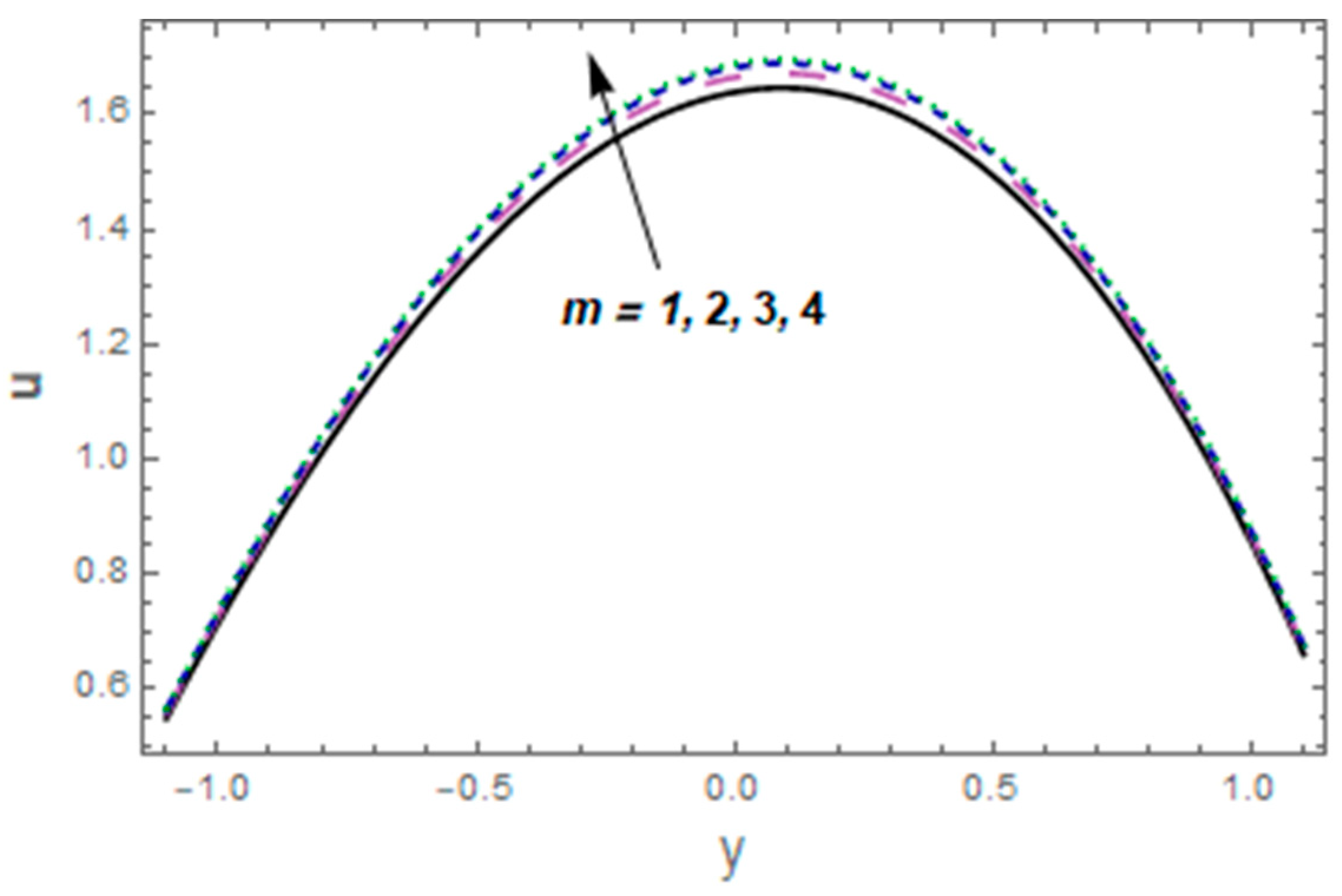
Figure 5.
Consequences of on where .

Figure 6.
Consequences of for where .

Figure 7.
Consequences of for where .

Figure 8.
Consequences of for where .
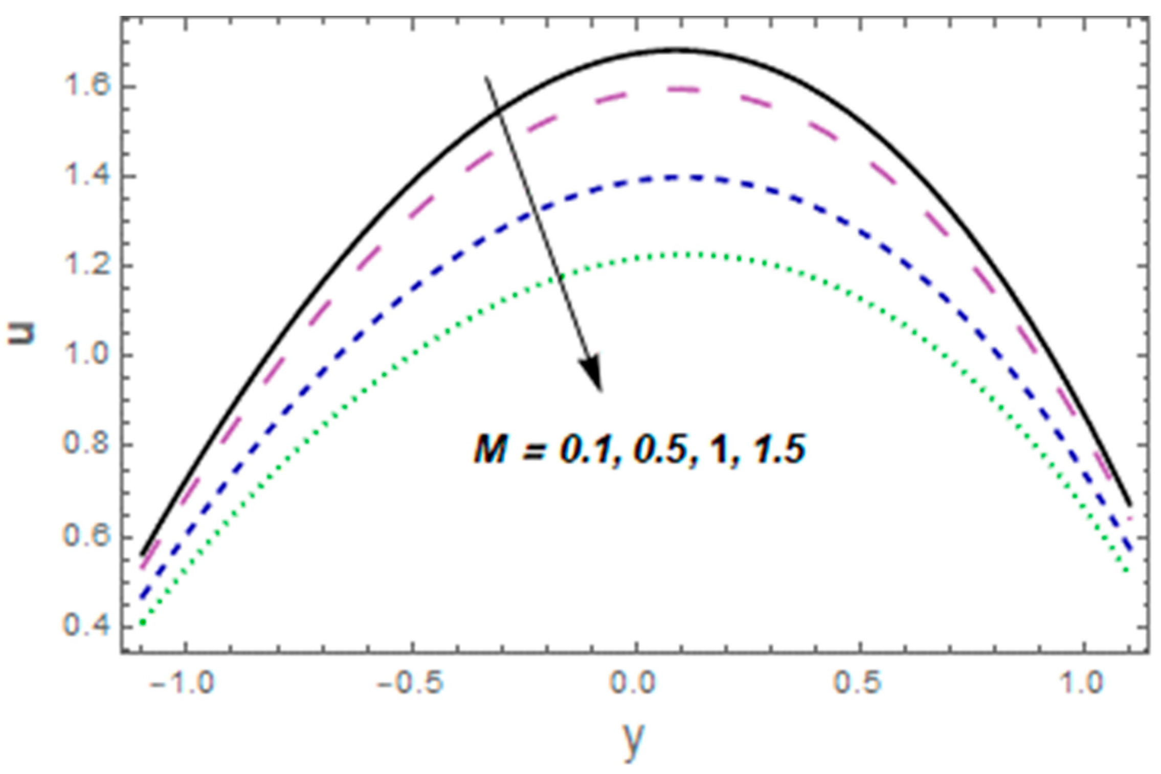
Figure 9.
Consequences of for where .
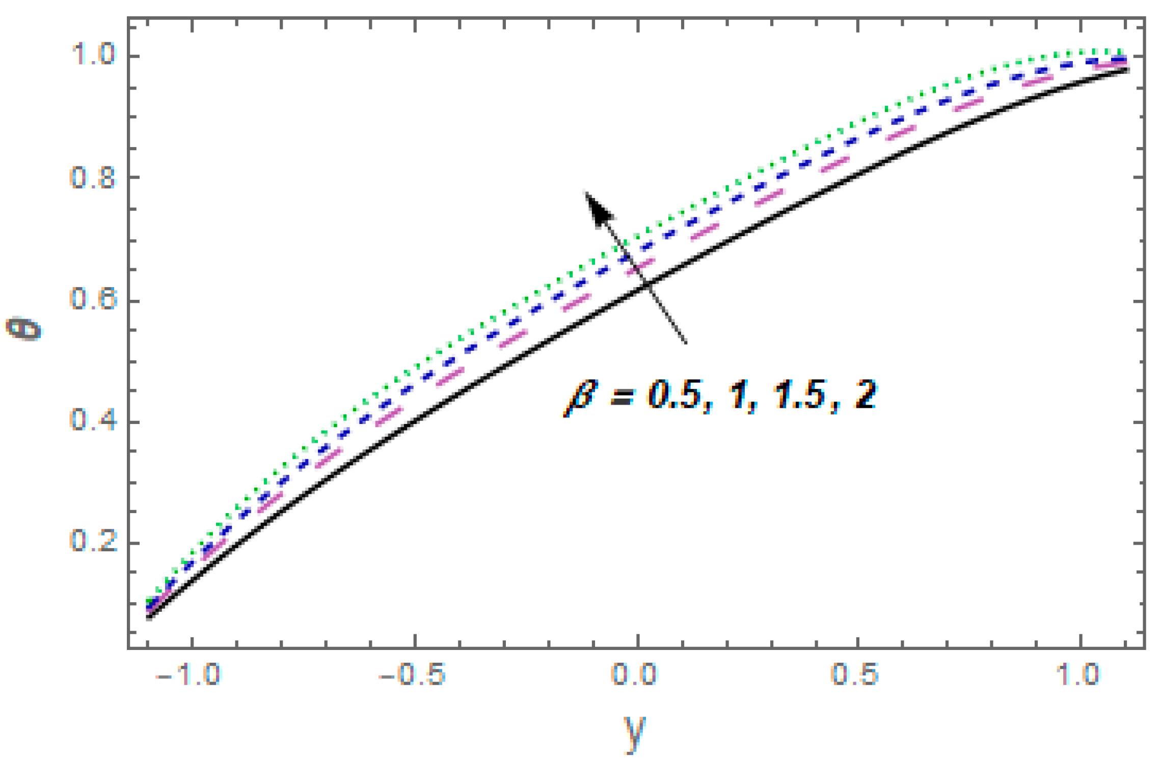
Figure 10.
Consequences of for where .
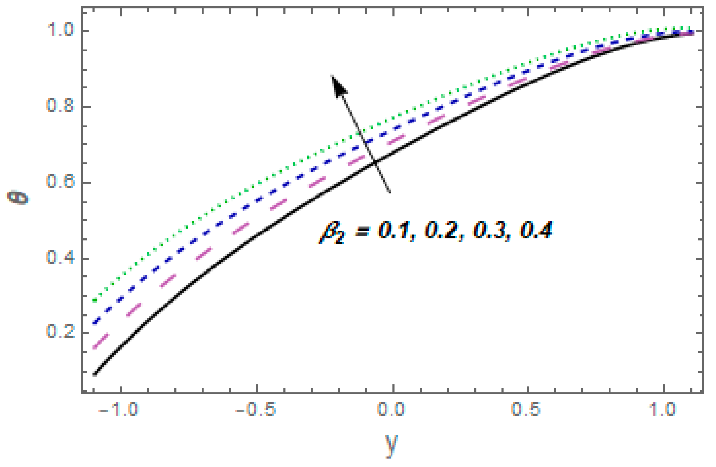
Figure 11.
Consequences of Br for where .
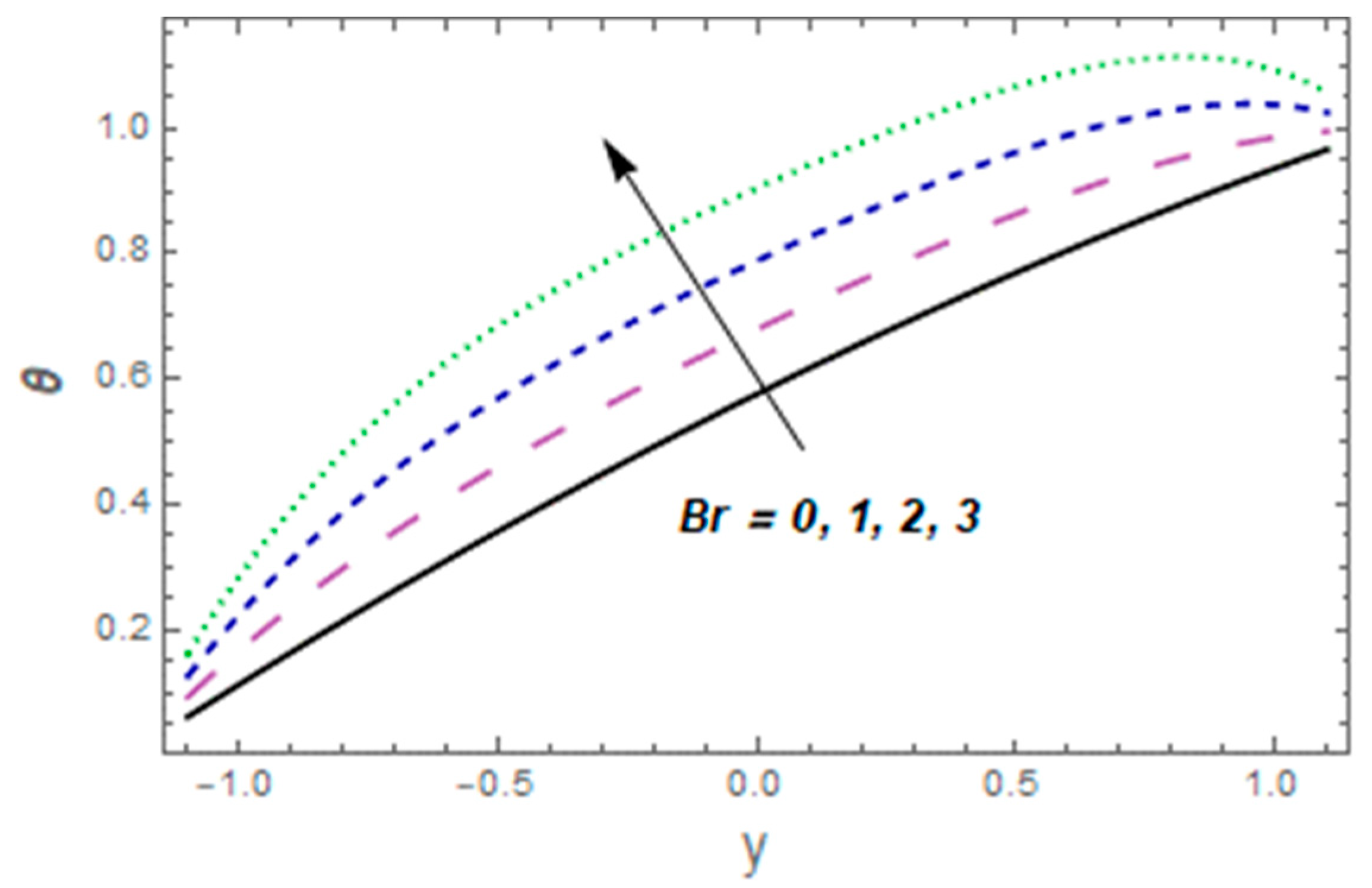
Figure 12.
Consequences of for where .
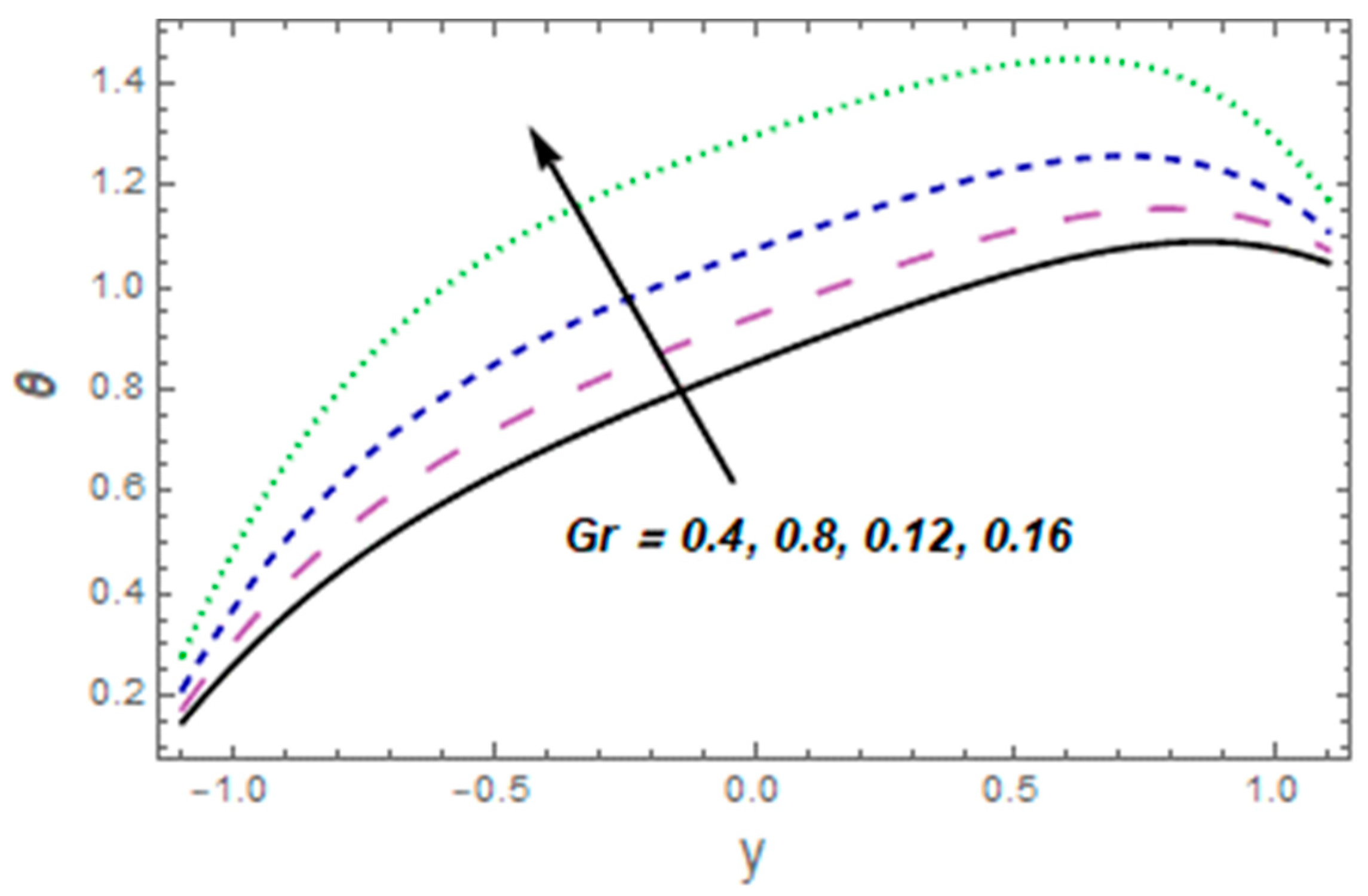
Figure 13.
Consequences of for where .
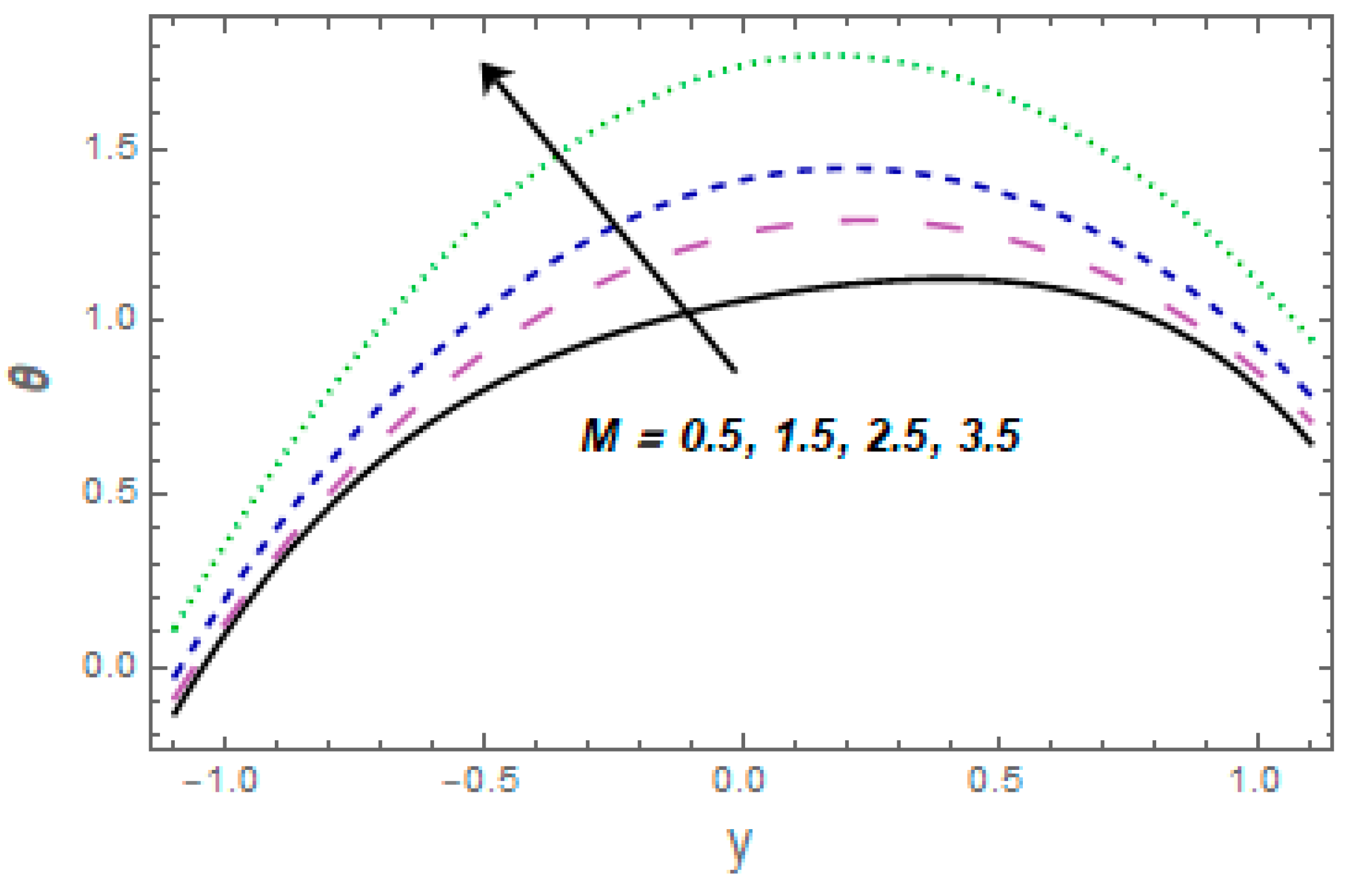
Figure 14.
Consequences of for where .

Figure 15.
Consequences of for where .
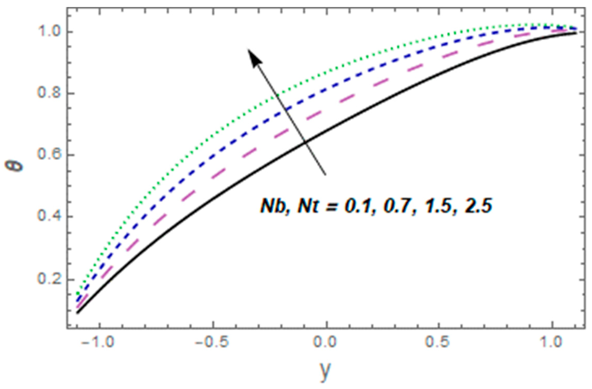
Figure 16.
Consequences of for where .
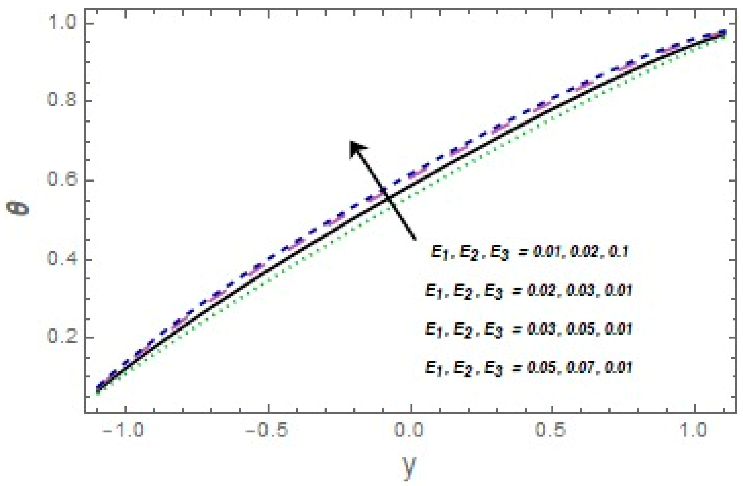
Figure 17.
Consequences of for where .
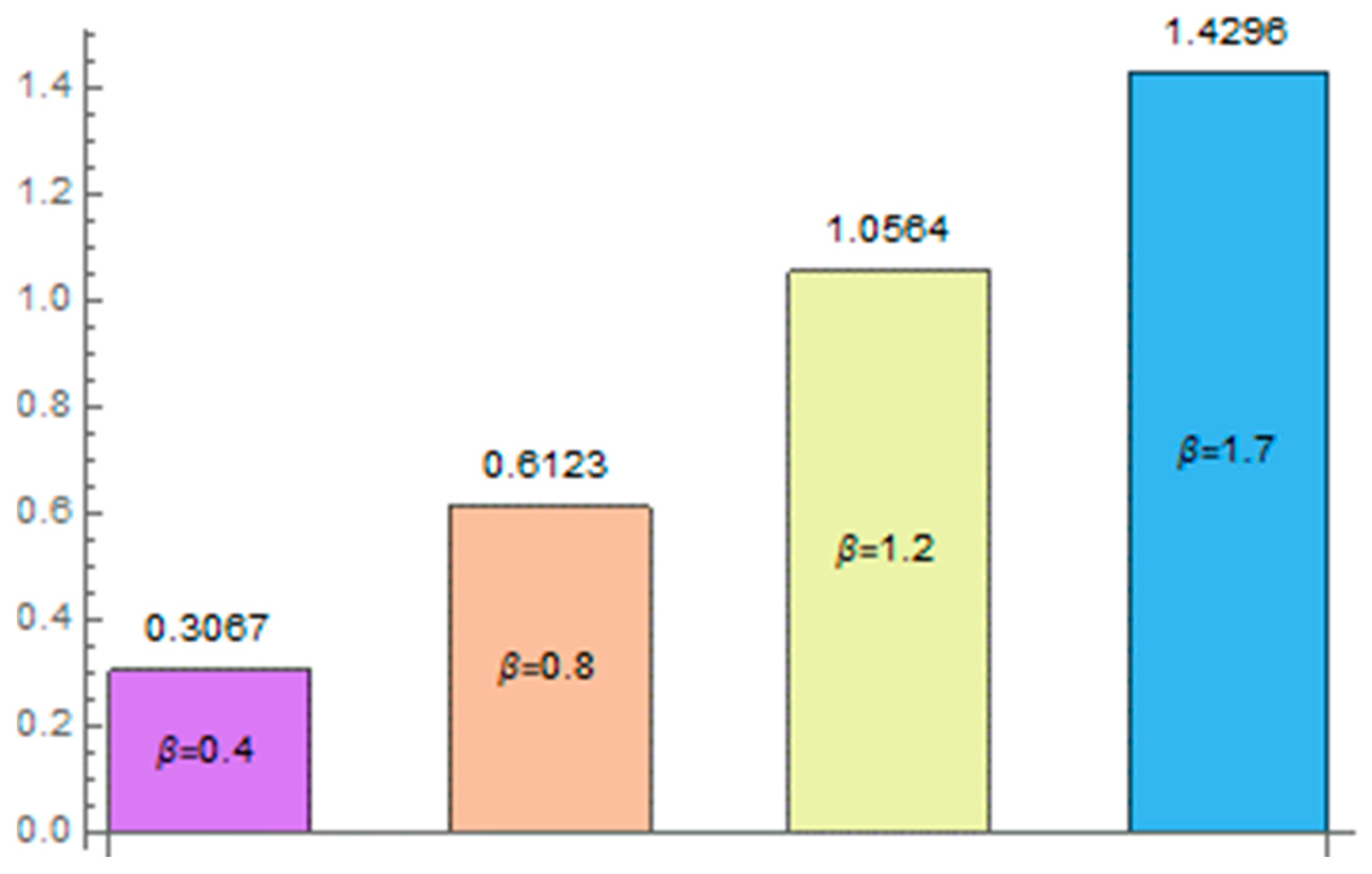
Figure 18.
Consequences of for where .

Figure 19.
Consequences of for where .

Figure 20.
Consequences of for where .
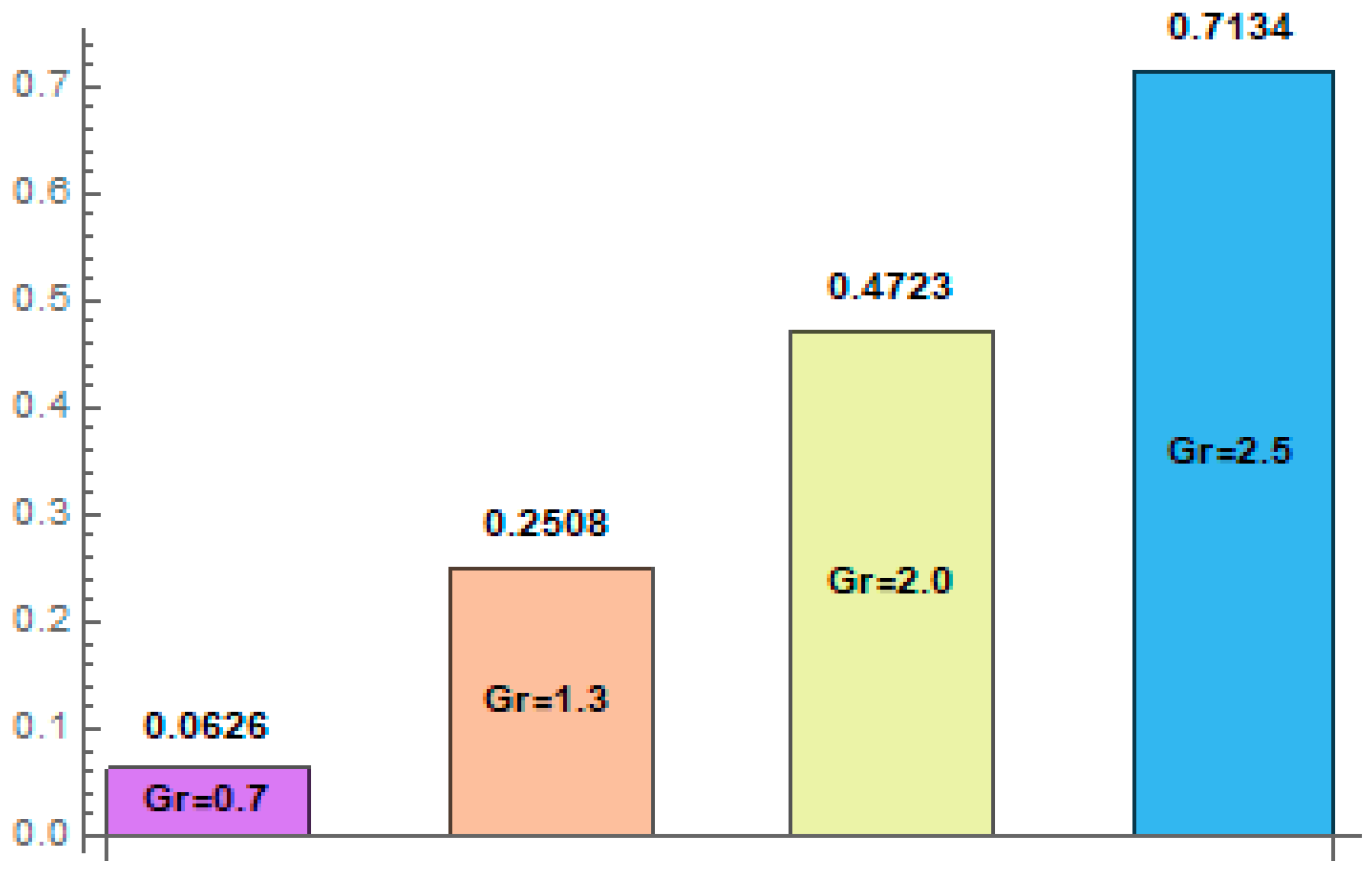
Figure 21.
Consequences of for where .

Figure 22.
Consequences of for where .
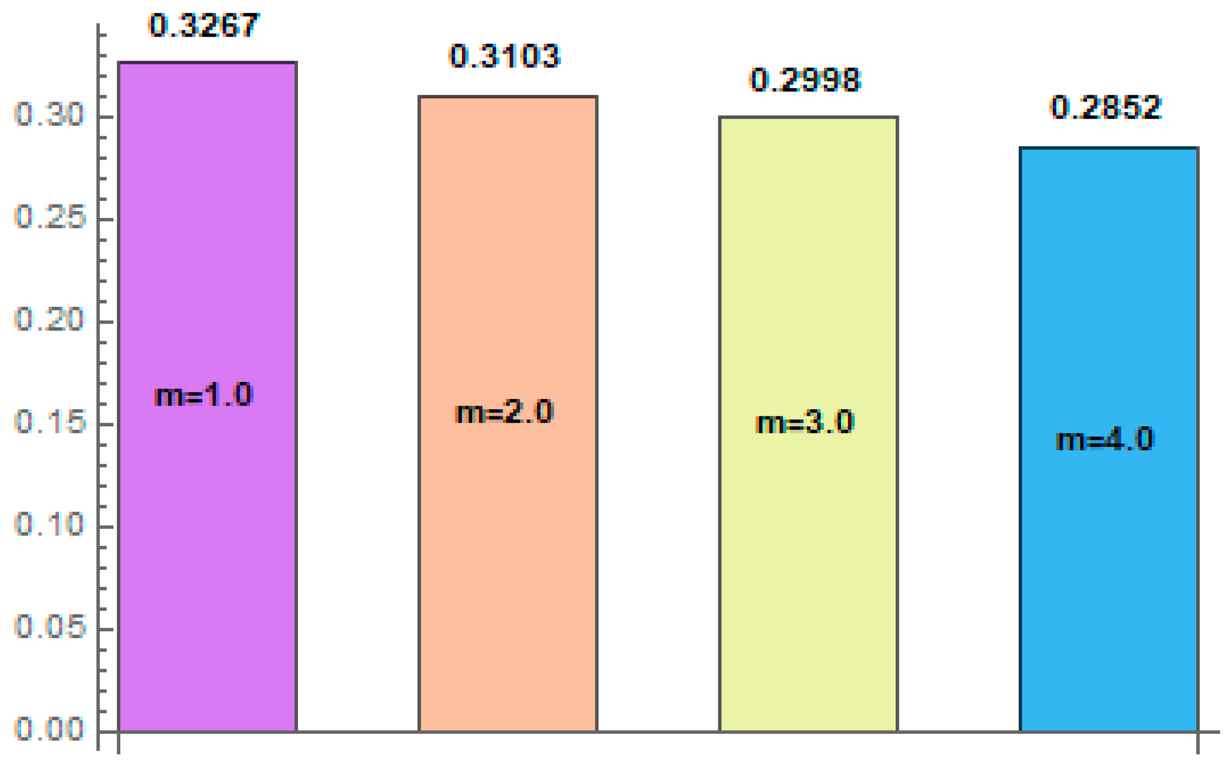
Figure 23.
Consequences of for where .

Table 1.
Effects of physical parameters on where .
| Parameters | Concentration | |||||
|---|---|---|---|---|---|---|
| 0.1 | 0.7 | 0.5 | 1 | 0.1 | 0.5 | 0.2484573 |
| 0.3 | 0.7 | 0.5 | 1 | 0.1 | 0.5 | 0.1952146 |
| 0.1 | 1 | 0.5 | 1 | 0.1 | 0.5 | 0.2464970 |
| 0.1 | 1.5 | 0.5 | 1 | 0.1 | 0.5 | 0.2430272 |
| 0.1 | 0.7 | 0.9 | 1 | 0.1 | 0.5 | 0.2365245 |
| 0.1 | 0.7 | 1.5 | 1 | 0.1 | 0.5 | 0.2226838 |
| 0.1 | 0.7 | 0.5 | 2 | 0.1 | 0.5 | 0.1589335 |
| 0.1 | 0.7 | 0.5 | 3 | 0.1 | 0.5 | 0.1100197 |
| 0.1 | 0.7 | 0.5 | 1 | 0.2 | 0.5 | 0.2265843 |
| 0.1 | 0.7 | 0.5 | 1 | 0.3 | 0.5 | 0.2076794 |
| 0.1 | 0.7 | 0.5 | 1 | 0.1 | 0.7 | 0.2152228 |
| 0.1 | 0.7 | 0.5 | 1 | 0.1 | 1 | 0.2209559 |
Table 2.
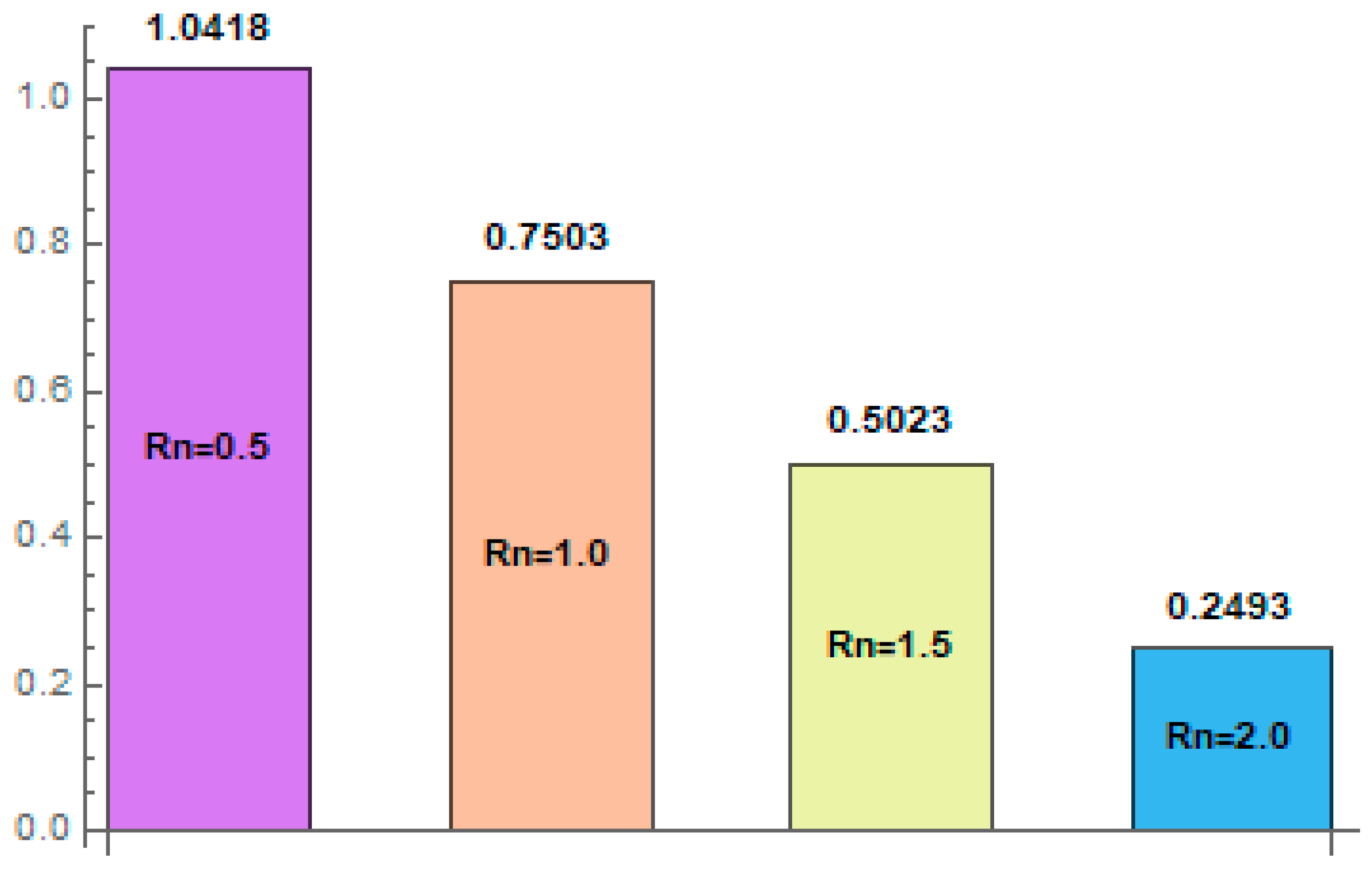
Comparison of numerical results with ref. [5].
Disclaimer/Publisher’s Note: The statements, opinions and data contained in all publications are solely those of the individual author(s) and contributor(s) and not of MDPI and/or the editor(s). MDPI and/or the editor(s) disclaim responsibility for any injury to people or property resulting from any ideas, methods, instructions or products referred to in the content. |
© 2023 by the authors. Licensee MDPI, Basel, Switzerland. This article is an open access article distributed under the terms and conditions of the Creative Commons Attribution (CC BY) license (https://creativecommons.org/licenses/by/4.0/).
Share and Cite
MDPI and ACS Style
Yasmin, H.; Nisar, Z. Mathematical Analysis of Mixed Convective Peristaltic Flow for Chemically Reactive Casson Nanofluid. Mathematics 2023, 11, 2673. https://doi.org/10.3390/math11122673
AMA Style
Yasmin H, Nisar Z. Mathematical Analysis of Mixed Convective Peristaltic Flow for Chemically Reactive Casson Nanofluid. Mathematics. 2023; 11(12):2673. https://doi.org/10.3390/math11122673
Chicago/Turabian StyleYasmin, Humaira, and Zahid Nisar. 2023. "Mathematical Analysis of Mixed Convective Peristaltic Flow for Chemically Reactive Casson Nanofluid" Mathematics 11, no. 12: 2673. https://doi.org/10.3390/math11122673
Note that from the first issue of 2016, this journal uses article numbers instead of page numbers. See further details here.