Abstract
It has been more than a decade since sequential indicator simulation was proposed to model geological features. Due to its simplicity and easiness of implementation, the algorithm attracts the practitioner’s attention and is rapidly becoming available through commercial software programs for modeling mineral deposits, oil reservoirs, and groundwater resources. However, when the algorithm only uses hard conditioning data, its inadequacy to model the long-range geological features has always been a research debate in geostatistical contexts. To circumvent this difficulty, one or several pieces of soft information can be introduced into the simulation process to assist in reproducing such large-scale settings. An alternative format of Bayesian sequential indicator simulation is developed in this work that integrates a log-linear pooling approach by using the aggregation of probabilities that are reported by two sources of information, hard and soft data. The novelty of this revisited Bayesian technique is that it allows the incorporation of several influences of hard and soft data in the simulation process by assigning the weights to their probabilities. In this procedure, the conditional probability of soft data can be directly estimated from hard conditioning data and then be employed with its corresponding weight of influence to update the weighted conditional portability that is simulated from the same hard conditioning and previously simulated data in a sequential manner. To test the algorithm, a 2D synthetic case study is presented. The findings showed that the resulting maps obtained from the proposed revisited Bayesian sequential indicator simulation approach outperform other techniques in terms of reproduction of long-range geological features while keeping its consistency with other expected local and global statistical measures.
MSC:
62C10
1. Introduction
High-quality probabilistic modeling of categorical variables (e.g., geological domains based on lithological description) is a vital demand in many geoscience disciplines, as it provides the basement for modeling the continuous variables (e.g., grade of elements and properties of rock) throughout the domain of study. This modeling process offers several applications in mineral resource estimation [1,2], statistic reservoir modeling [3,4], and modeling of aquifers in hydrogeology [5], to name a few. To model the categorical variables, among others, truncated Gaussian simulation [6,7], plurigaussian simulation [8,9], multiple-point statistics [5], and sequential indicator simulation [10,11,12] received significant attention for building such categorical models. The latter, modeling of a continuous variable, is more popular due to its simplicity and straightforwardness, and the algorithm itself is available in several commercial software programs. The resulting models are acceptable where there are no large-scale geological patterns. However, in the case of having curvilinear or long-range geological features, the algorithm produces very patchy and unstructured results, which is a legitimate criticism of this method [13,14]. The reason is that sequential indicator simulation only takes into account the two-point statistical measures of the geological domains that are informed by hard data. To solve this issue, several variations of sequential indicator simulation have been developed that consider the soft information as secondary data to inform the large-scale geological variability at the target simulation nodes, which substantially improves the applicability of the method. In this context, hard and soft data refer to measured values at the borehole via the sampling points and interpretive geological models at target grid nodes, respectively.
A possible solution to include secondary/soft information in the process of simulation is to use the probability aggregation concept [15]. A proper evaluation of different probability aggregation methods with special attention to their applicability using geoscientific data is conducted by Allard et al. [16]. They showed that the log-linear pooling outperforms the linear pooling when integrating them with the truncated Gaussian and the Boolean models in geostatistics. The integration of log-linear pooling in several geostatistical algorithms has already been developed for various applications: interpolation of satellite images [17], 3D multiple-point statistics using 2D training images [18], multiple-point geostatistical simulations using secondary exhaustive information [19], and Bayesian sequential Gaussian simulation for modeling the continuous hydrogeophysical data [20].
Probability aggregation is also employed specifically in sequential indicator simulation. Among others, Bayesian sequential indicator simulation [21] was introduced to integrate a simple Bayesian updating rule to construct a local posterior distribution of the geological domains at the target grid node. This work was developed to model the lithofacies in static reservoirs where the soft data can be informed by seismic attributes for the different lithofacies. Another form of Bayes’ law was introduced by Ortiz and Deutsch [22], where the indicator formalism in this sequential simulation technique is updated by using the multiple-point configuration of the soft data. The method is proposed to simulate the continuous variable in the context of mineral resource estimation, where the soft conditional probability is advised by using the production data such as blasthole. However, in these methods, the hard and soft data use equal constant weights, meaning identical influence on the final simulation results. To overcome this limitation, a revised version of Bayesian sequential indicator simulation is proposed in this study for the purpose of modeling the categorical variables (e.g., geological domains) that are integrated with a log-linear pooling approach. The soft information in this enhanced process of simulation is inferred from an interpolation technique using only the hard conditioning data at the sampling point.
2. Sequential Indicator Simulation
2.1. Conventional Sequential Indicator Simulation
Sequential indicator simulation [10,11,12] is a stochastic methodology for modeling Μ categories, for which they are exhaustive and mutually exclusive at all data locations. This means that one of the categories must predominate at each individual sample point.
In order to perform a sequential indicator simulation algorithm, first, the categorical variable through the hard conditioning data at sample locations is transformed into a matrix of hard indicator variables, characterized as:
In this equation, predominating category at location that is converted to indicators necessitates that .
In the second step, a random path is identified to visit each node of the target grid only once. The next step is to estimate the corresponding category at randomly selected target node grid node , using the indicators that are obtained through Equation (1) at hard conditioning data. There are different methodologies in geostatistics that can be utilized for this purpose. Among others, the simple kriging method provides promising results. This geostatistical interpolation paradigm is built based on three constraints [23]: (a) the estimator is a weighted linear combination of the available hard data (linearity constraint), (b) the estimator is unbiased, that is, the expectation of the error is 0 (unbiasedness constraint), and (c) the error variance is minimum (optimality constraint). The first restriction necessitates writing the estimator as a linear combination (weighted average) of the neighboring hard data to estimate the variable of interest at target grid node :
where data are composed of neighboring hard conditional data; is the global declustered mean value of the corresponding variable , is the weights assigned to the variable at the location . The weights needed in Equation (2) are achievable by solving a covariance matrix for each as:
where is the covariance of variable . Solving the kriging system in Equation (3) to obtain the weights requires the knowledge of covariance of variable . In this respect, the lineal model of regionalization is widely used to fit such covariances, owing to its mathematical simplicity and tractability [9,23]. In this model, the covariance is defined as weighted sum of basic covariances, also called basic nested structures:
where for each structure , is the positive sill of basic permissible covariance model .
Therefore, one can use the simple kriging paradigm to estimate the corresponding category at the target grid node. Since the initial data is already converted to indicators, then the aim of simple kriging in this step is to establish the conditional probability of occurrence of each indicator at the corresponding target grid node :
where data are composed of neighboring hard conditional indicators and previously simulated indicator values; the is the global declustered proportion of each category (i.e., prior probability or prior proportion), which equivalently can be defined as ; is the weights assigned to the indicator variable at the of this indicator variable. The weights needed in Equation (5) are achievable by solving a covariance matrix for each using Equation (3). Then, the permissible model of can be inferred from the direct calculation of covariance over each indicator variable or it can be deduced from the calculation of variogram over indicator variable . In this case, the variogram can then be converted to covariance to be embedded into Equation (3) for computing the corresponding weights .
Since each category is independently estimated, an order relation deviation is expected for the estimated conditional probabilities. This signifies that the probabilities do not always sum to one, and the existence of negative probabilities is expected. The reason is that some of the weights obtained by solving the simple kriging system via Equation (3) receive negative or high values. These particular weights lead to producing some negative values or very high values for estimated indicators, which are more than 1 [24,25,26]. Then, in the fourth step, the deviations in probabilities for order relation should be rectified [26]. In this respect, one can utilize the bounds correction, signifying that all negative estimated values are set to 0, and all high values (more than 1) are set to 1. Then, a normalization of probabilities is needed to force the summation of all estimated conditional probabilities to reach 1 at all target grid nodes [23]. Once the probabilities of each indicator are estimated and their order related problems are corrected, then one can define any ordering of the categories and build a cumulative distribution function (cdf-type function). Afterward, the fifth step includes drawing a random number from a uniform distribution in by Monte Carlo simulation. Therefore, the simulated category at location can be obtained with an inverse of the quantile associated with that generated random number in . In the sixth step, the simulated value is added to the hard conditioning data, and then the algorithm proceeds to the next target node, following the identified random path, repeating steps from one to five. In order to generate another realization , with total number of realizations, one needs to repeat the entire algorithm with a different random path. These simulated values are obtained by only hard conditioning data- . However, the current methodology is poor in reproduction of connectivity or large-scale geological features between sample points. In the following, we show how soft information can be incorporated to simulate the values at target nodes, enforcing the connectivity in the outcomes.
2.2. Revisited Bayesian Sequential Indicator Simulation
If the secondary evidence, known as soft information, is available at the target node , the conditional probability of occurrence of each category obtained from Equation (5) can be updated accordingly. Let us denote event a category that needs to be simulated at target grid node, and represent information of that underlying category, for which they are inferred by using the hard conditioning data, soft data, or any other source of information. Indeed, we aim at approximating the probability based upon the coexisting information of the conditional probabilities. Probability aggregation [16] is used to construct an approximation of the true conditional probability by utilizing an aggregation operator , which is also known as the pooling operator or pooling formula:
In the case of having a prior probability for the category sought, then Equation (6) can be generalized to:
Among others, aggregation operators based on the multiplication of probabilities appear to be more suited in geoscience than those formulated based on an addition operator (Allard et al. 2012). These product-based pooling operators are linear operators of the logarithms of the probabilities [16]:
where is a normalizing constant. This expression equivalently can be converted to the multiplication of probabilities:
where are positive weights with restriction to verify external Bayesianity. In Equation (9), there is no restriction on the weights.
In the context of sequential indicator simulation using the secondary data, subject to having one hard conditioning data and one soft information , log-linear pooling can be simplified to combine the information provided by these two sources of information:
where is prior probability of each category ; and are the weights that can be arbitrary assigned to the hard and soft data, and is always verified.
Therefore, the conditional probability of occurrence of each category obtained from Equation (5) can be updated by using Equation (10) as:
where is soft information, for which its conditional probability of occurrence of category can be reported from an interpretive geological block model at the target grid node. For instance, wireframing or hand contouring can provide such a geological block model [2]. However, it is somehow tedious to produce such a probabilistic information from a deterministic interpretive model of geological domains in the region of study. There is an alternative way to convert this deterministic model to conditional probabilities, as thoroughly explained in [27]. In this study, we propose to obtain values from simple kriging of the indicators at hard conditioning data. These estimated values provide probabilistic information of the occurrence of that category at the corresponding target grid node . However, to obtain , we take both the neighboring hard conditional indicator data and also the previously simulated indicator values as a typical practice in conventional sequential indicator simulation as explained in Section 2.1. In practice, the soft information in this probability aggregation method helps improve the conventional sequential indicator simulation for better reproduction of long-range geological structures. The most important issue in this approach is to properly assign the weights of hard and soft data . In the case of and , Equation (11) simplifies to the traditional Bayesian sequential indicator simulation as proposed in [21].
2.3. Optimal Evaluation of Weighting Mechanism
The proposed log-linear pooling approach in Equation (10) allows one to identify different or equal weighting schemes for a specific category that are coming from different sources of information. These are prior proportion, primary (hard) and secondary (soft) data, where their weights can dictate the intensity of their influence in the final probability aggregation resulting through Equation (11). The proposed methodology in this work highly depends on the proper assignation of these weights so that their improper designation yields completely different results. These weights can be either assigned equally or ranked differently, for instance, based on the opinion of an expert. Allard et al. [16] suggested using a log-likelihood approach to optimally identify these weights. Nassbaumer et al. [20] proposed a multi-step sophisticated approach to change the weights multiple times during the simulation process following a Monte Carlo-type search. In this study, we used an empirical technique to assign the weights that gradually change in the interval of , allowing the testing of our algorithm conveniently. The algorithm for identification of optimal weights is as follows:
- Testing the algorithm with 24 different experiments of and as provided in Table 1.
 Table 1. Twenty-four experiments based on different weighting schemes of and ; introduces the weight of prior proportion for the category sought.
 - Evaluating the performance of the experiments by calculating the error in the reproduction of the proportion of indicators.
- Evaluating the performance of the experiments by calculating the error in matching percentage with the reference map.
- Evaluating the performance of the experiments by calculating the error in the reproduction of connectivity measures of the categories.
- Evaluating the performance of the experiments by calculating the error in the reproduction of spatial continuity of the categories.
- Fitting polynomial function to interpolate the errors.
- Obtaining the optimal weights based on minimum error.
In the above criteria, reproduction of proportions refers to the examination of reproduction of in the simulation results. Connectivity measures is defined as the probability that two target grid nodes belonging to category are connected [28]:
where is a non-decreasing function as increases. The connectivity function can be estimated by:
where is the estimate of connectivity function for distance , the number of target grid nodes, separated by a vector of distance , that belong to category and are connected and the number of target grid nodes, deparated by a vector of distance , that belong to category and that may or may not be connected.
Concerning the spatial continuity evaluation, a variogram can be a satisfying measurement. To do so, experimental variogram computes the average dissimilarity between data separated by vector . It is calculated as half the average difference between components of every data pair [9,29]:
where is a d-increment of the indicator variable and is the number of pair.
Through the synthetic case study, we show how the method proposed does work and how these weights can be optimally identified.
3. Results
3.1. Synthetic Case Study
To test the proposed methodology and evaluate the optimal weighting parameters, a synthetic case study is considered. For this purpose, one categorical variable, including two indicators/categories, is non-conditionally simulated on a 2D 300 m × 300 m domain consisting of 300 × 300 nodes by using plurigaussian simulation [8] associated with an anisotropic spatial continuity. Ten realizations are produced, and the one (reference map hereafter) is selected in such a way that it shows long connectivity along easting and relatively short connectivity along elevation coordinates (Figure 1A). In order to mimic the vertical sampling pattern like the ones in the actual case studies, 100 points are randomly sampled from the reference map along elevation to constitute four synthetic boreholes throughout the domain. However, in order to evaluate the algorithm properly, two target areas are of paramount importance. These are identified by two ellipses (I and II) in Figure 1A. In fact, we are interested in producing the realizations that honor the connectivity of the categories through these two critical areas when there are few hard conditioning data points. Therefore, it was intended to sample only one category per each of these two-target areas (Figure 1B). The lack of data in these two areas can be an excellent signature for evaluating the proposed method. Consequently, this synthetic dataset is used in the proposed algorithm to compare the simulation results with a reference map to provide evaluation debates.
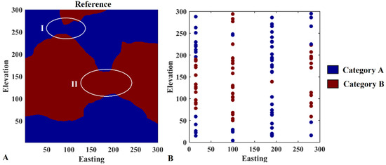
Figure 1.
Reference dataset, (A) reference map, (B) synthetic sampled dataset; only one sample is preserved in the target areas I and II to better evaluate the revisited Bayesian sequential indicator simulation in this study.
The connectivity on the selected map, to be considered a reference map, is also verified by computing the connectivity functions [23] over this realization along the specified coordinates (Equation (13)).
As can be observed from Figure 2, there is approximately 50% and 0.0% probability that categories A and B are connected from west to east and from south to north, respectively. This interpretation is obtained by looking at the connectivity measures at large lag distances when they reach a steady range around the lag of 240. This is also compatible with the visual inspection of the map illustrated in Figure 1A. Therefore, this is an interesting reference map for further analysis in this study.
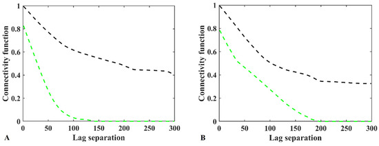
Figure 2.
Connectivity measures along Easting (back dashed line) and Elevation (green dashed line) for (A) category A, and (B) category B.
Once the synthetic sampling points are identified, the next step in the proposed algorithm is to produce a map that reports the soft data at target nodes to be used subsequently for log-linear pooling probability aggregation in revisited Bayesian sequential indicator simulation through Equation (6). In this study, simple kriging is used to map the soft information for each indicator. Therefore, after variogram analysis, the categories/indicators are estimated on the target grid nodes using up to 40 conditioning data in a moving neighborhood configuration (Figure 3). Due to the existence of indicator value at synthetic sample points, these maps are deemed as the probability of occurrence of the corresponding category at the target node, for which they can be used as soft information in Equation (7). One advantage of this map is that one can recognize the probability of connectivity between the boreholes, which is favorable information for modeling the categories with long connectivity.
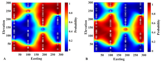
Figure 3.
Probability of occurrence of (A) category A and (B) category B obtained by estimating the conditioning indicator data on the target grid nodes. These maps are used as soft information in the proposed algorithm.
The next step in the revisited Bayesian sequential indicator simulation in this study is to implement the simulation algorithm but using updating scheme of Equation (11) to update the probability of occurrence of the corresponding category . As mentioned earlier, the updated probability highly depends on the assignation of weights and . A method is used to test different weighting schemes in Equation (11) to evaluate the optimum weighting values in the revisited Bayesian sequential indicator simulation. In this technique, and , and the prior proportion ranging with a weight of . These 24 trials are shown in Table 1.
In this examination, the trials with and , signify that the revisited Bayesian sequential indicator simulation is only based on the soft information (pure soft simulation hereafter). Those trials with and , denote that the resulting revisited Bayesian sequential indicator simulation is solely yielded on the hard conditioning data (pure hard simulation hereafter). The trial represents the conventional sequential indicator simulation with and . The trial providing the simulation results with and presents the traditional Bayesian Updating approach as proposed in Doyen et al. [21] (Doyan’s simulation hereafter). There are some links between Doyan’s simulation and sequential indicator simulation that uses a collocated cokriging by different implementation mechanisms [13]. All these subgroups are some special cases of the revisited Bayesian sequential indicator simulation as proposed in this study. However, in order to be clearer about these subgroups, another subgroup is defined, which is called Revisited Bayesian simulation hereafter, for which and vary between {0, 2} and {0.5, 2}, respectively, but excluding the weights belonging to pure soft simulation, pure hard simulation, traditional simulation, and Doyan’s simulation. A summary of these techniques is provided in Table 2. A note is also provided in Table 1 to link the trials in Table 1 to the subgroups in Table 2.
Table 2.
Comparison of some key properties of the log-linear pooling aggregation approach in this study; weight of the prior proportion for the category sought is .
Implementation of simulation for all the trials was conducted under a moving neighborhood scheme with up to 40 hard conditioning data and 40 previously simulated data. The sequential paradigm is followed a random sequence while using a multiple-grid simulation procedure. The number of realizations is 100. Some realizations from each subgroup (presented in Table 2) are selected for visualization (Figure 4). The rest of the realizations for the other trials are provided in Appendix A (Figure A1). As can be seen, the results obtained by using only pure soft information dramatically failed in reproducing the shape of both categories A and B, which do not show the underlying structure. In pure hard simulation, when , the resulting maps are quite patchy (Figure 4B). However, by increasing the weight of hard data, the shape of category B, to some extent, is regenerating. It can be seen that the reproduction of connectivity is highly controlled by the weight assigned to soft data (Figure 4D,F). One of its particular cases is the one with and (Figure 4F), where it shows the result of traditional sequential indicator simulation. The shape of category B on the left and on the right sides is more or less reproduced, but the continuity of category B is disconnected around area II, shown by a white ellipse in Figure 4A. This is a typical problem of traditional sequential indicator simulation, in which the geological features with long connectivity cannot be produced properly. Doyan’s simulation, which represents conventional Bayesian updating in Equation (11), could produce the general shape of category B in the places where enough conditioning data are available, but again it failed to produce the connectivity of interest in area II (Figure 4E). In these figures, the revisited Bayesian simulation with and seems to be the most promising one among others.
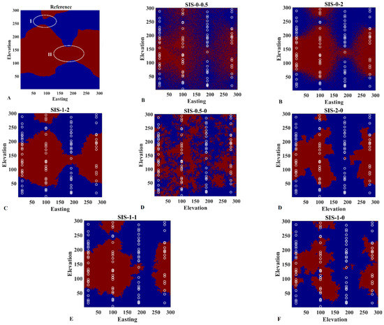
Figure 4.
Comparison of (A) reference map with resulting simulation maps obtained from (B) pure soft simulation, (C) revisited Bayesian simulation, (D) pure hard simulation, (E) Doyan’s simulation, and (F) traditional simulation.
3.2. Validation
However, the results depicted in Figure 4 are only one single realization of each trial, and one might be interested in examining the probability maps obtained from 100 realizations that assess the uncertainty in the categories at a local (node-by-node) scale for better validation. The maps are constructed by calculating, for each grid node, the frequency of occurrence of category B over 100 conditional realizations (Figure 5). They constitute a complement to the reference map insofar as they show the risk of finding a category different from the one that has been expected. The sectors with little uncertainty are those associated with a high probability for a given category (painted in red in Figure 5), indicating that there is little risk of not finding category B, or those associated with a very low probability (painted in dark blue in Figure 5), indicating that one is pretty sure of not finding this category, while the other sectors (painted in light blue, green or yellow in Figure 5) are more uncertain. As can be observed, the revisited Bayesian simulation method with and provides the most prominent results to give the high probability of connectivity close to areas I and II, as we expect from the reference map. The rest of the probability maps are presented in Appendix B (Figure A2).
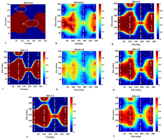
Figure 5.
Comparison of (A) reference map with resulting simulation maps obtained from (B) pure soft simulation, (C) revisited Bayesian simulation, (D) pure hard simulation, (E) Doyan’s simulation, and (F) traditional simulation.
From the probability maps, one can build a categorical map by selecting, for each grid node, the most probable category. This model can then be compared to the reference map in order to identify the grid nodes for which the category matches the most probable one and also the grid nodes for which there is a mismatch (Figure 6). The latter grid nodes are mostly located near the border of the two categories. As can be observed, revisited Bayesian simulation (Figure 6C) and traditional simulation (Figure 6E) provided better results compared to other experiments.
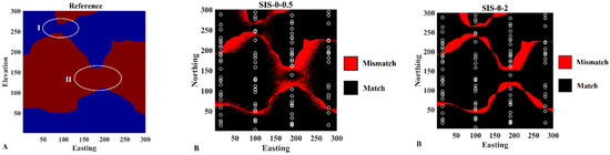
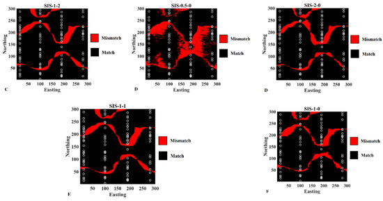
Figure 6.
The matches and mismatches with respect to (A) reference map for resulting simulation maps obtained from (B) pure soft simulation, (C) revisited Bayesian simulation, (D) pure hard simulation, (E) Doyan’s simulation, and (F) traditional simulation.
3.3. Assessment of Optimal Weights
It is shown that the revisited Bayesian simulation method with weights and , by visual inspection, can deliver the most promising results compared to the reference dataset; this has been achieved qualitatively by using only the realizations and probability maps. To show this also quantitatively, a validation step is performed to assess the accuracy of the obtained weights. To secure the optimum weights of and four criteria were assessed by calculating the error deducing from:
- (A)
- The difference between the reproduced proportion of indicators through the realizations and the proportion of categories/indicators in the reference map.
- (B)
- The difference in the percentage of the match [27] between the most probable categorical map and the reference map.
- (C)
- The difference between the connectivity function of each indicator and the connectivity function in the reference map.
- (D)
- The difference between the variogram reproduction of the indicators and the original variogram of the indicators in the reference map.
In all these criteria, the underlying parameter is calculated over individual realizations, and then it is averaged. The average value is compared with the original parameter obtained from the reference map. The difference (error) is then taken into account as the main criterion for evaluating the optimal weights of and . For each criterion, 24 experiments are available, where their errors are calculated. Different polynomial functions are tested to interpolate the errors within the trials. The one is selected for each that offers the highest .
As can be seen from Figure 7, there are two optimal weight candidates that worth to be discussed. It seems that when the is equal to 1 and 1.5, and is equal to 2, the errors in variogram reproduction along Easting (Figure 7G), connectivity for both categories (Figure 7C,E), and slightly variogram reproduction along Northing (Figure 7H) are quite low and almost equivalent. However, this is not true when one considers the errors in proportion reproduction (Figure 7A), match percentage (Figure 6B), and northing connectivity for both categories (Figure 7D,F). The individual realizations and the probability maps obtained from these two weights (Appendix A) also corroborated these quantitative findings. Therefore, these numerical examinations also verified that and are two optimal weights for the corresponding probability aggregation in the proposed revisited sequential indicator simulation approach in this case study.
Figure 7.
Validation by computing the error for (A) Proportion reproduction, (B) Match percentage, (C) Easting connectivity-R1, (D) Northing connectivity-R1, (E) Easting connectivity-R2, (F) Northing connectivity-R2, (G) Variogram-Easting, (H) Variogram-Northing; weight-hard data ( and weight-soft data .
4. Discussion and Conclusions
A methodology proposed in this study revisits the traditional Bayesian sequential indicator simulation. This versatile model uses a log-linear pooling probability aggregation approach to integrate the probabilities that are coming from different sources. The algorithm makes the job easier to find the soft information by using only an available geostatistical interpolation technique to inform the soft data at the target data location. Different weighting options were also tested, and through a numerical examination, it was revealed that different weights that are assigned to each source of information produce different results. Indeed, the incorporation of sources of information with different influences was overlooked through all previously Bayesian sequential indicator simulation approaches. The results of this study compared with traditional sequential indicator simulation algorithms, and it was shown that the long-range structures could be better produced. Nevertheless, the method proposed is not restricted to only two sources of information. Equation (5) can be generalized to include more sources of information, and the weights can simply be tuned. However, the methodology needs some numerical experiments to assess the optimal weights. Further research can focus on developing a sophisticated technique to infer the weights automatically. The proposed algorithm is tested in a synthetic case study, but it can also be tested in an actual case study. To set the optimal weights, one solution is to use the production dataset as a benchmark. This information may only be available partially in a domain. The obtained weights can be taken into account for resource reconciliation in other parts of the domain, where only exploratory data are available and one does not have access to production data. Another avenue of research can further develop the method to model the non-stationary domains.
Funding
This research was funded by Nazarbayev University via Faculty Development Competitive Research Grants for 2021–2023, grant number 021220FD4951.
Data Availability Statement
Not applicable.
Acknowledgments
The author acknowledges Nazarbayev University, particularly School of Mining and Geosciences, and Aizhan Nurakysheva for providing the financial open-access support of this work.
Conflicts of Interest
The author declares no conflict of interest.
Appendix A


Figure A1.
Realizations obtained from revisited Bayesian sequential indicator simulation by different assignations of weights.
Appendix B


Figure A2.
Probability maps obtained from revisited Bayesian sequential indicator simulation by different assignations of weights.
References
- Madani, N.; Maleki, M.; Emery, X. Nonparametric Geostatistical Simulation of Subsurface Facies: Tools for Validating the Reproduction of, and Uncertainty in, Facies Geometry. Nat. Resour. Res. 2019, 28, 1163–1182. [Google Scholar] [CrossRef]
- Rossi, M.E.; Deutsch, C.V. Mineral Resource Estimation; Springer: New York, NY, USA, 2014; p. 332. [Google Scholar]
- Sadeghi, M.; Madani, N.; Falahat, R.; Sabeti, H.; Amini, N. Hierarchical reservoir lithofacies and acoustic impedance simulation: Application to an oil field in SW of Iran. J. Pet. Sci. Eng. 2022, 208, 109552. [Google Scholar] [CrossRef]
- Pyrcz, M.J.; Deutsch, C.V. Geostatistical Reservoir Modeling; Oxford University Press: Oxford, UK, 2014. [Google Scholar]
- Mariethoz, G.; Caers, J. Multiple-Point Geostatistics: Stochastic Modeling with Training Images; Wiley: New York, NY, USA, 2014; p. 376. [Google Scholar]
- Matheron, G.; Beucher, H.; Galli, A.; Guérillot, D.; Ravenne, C. Conditional simulation of the geometry of fluvio-deltaic reservoirs. In Proceedings of the 62nd Annual Technical Conference and Exhibition of the Society of Petroleum Engineers, Dallas, TX, USA, 27–30 September 1987; pp. 591–599. [Google Scholar]
- Galli, A.; Beucher, H.; Le Loc’h, G.; Doligez, B. The pros and cons of the truncated Gaussian method. In Geostatistical Simulations; Armstrong, M., Dowd, P.A., Eds.; Kluwer: Dordrecht, The Netherlands, 1984; pp. 217–233. [Google Scholar]
- Madani, N. Plurigaussian Simulations. In Encyclopedia of Mathematical Geosciences; Encyclopedia of Earth Sciences Series; Daya Sagar, B., Cheng, Q., McKinley, J., Agterberg, F., Eds.; Springer: Cham, Switzerland, 2021. [Google Scholar] [CrossRef]
- Chilès, J.P.; Delfiner, P. Geostatistics: Modeling Spatial Uncertainty; Wiley: New York, NY, USA, 2012; p. 699. [Google Scholar]
- Alabert, F. Stochastic Imaging of Spatial Distributions Using Hard and Soft Information. Master’s Thesis, Department of Applied Earth Sciences, Stanford University, Stanford, CA, USA, 1987; p. 332. [Google Scholar]
- Journel, A.G.; Alabert, F.G. New method for reservoir mapping. J. Pet. Technol. 1990, 42, 212–218. [Google Scholar] [CrossRef]
- Journel, A.G.; Gómez-Hernández, J.J. Stochastic imaging of the Wilmington clastic sequence. SPE Form. Eval. 1993, 8, 33–40. [Google Scholar] [CrossRef]
- Deutsch, C.V. A sequential indicator simulation program for categorical variables with point and block data: BlockSIS. Comput. Geosci. 2006, 32, 1669–1681. [Google Scholar] [CrossRef]
- Emery, X. Properties and limitations of sequential indicator simulation. Stoch. Environ. Res. Risk Assess. 2004, 18, 414–424. [Google Scholar] [CrossRef]
- Genest, C.; Zidek, J.V. Combining probability distributions: A critique and an annotated bibliography. Stat. Sci. 1986, 1, 147–148. [Google Scholar]
- Allard, D.; Comunian, A.; Renard, P. Probability aggregation methods in geoscience. Math. Geosci. 2012, 44, 545–581. [Google Scholar] [CrossRef]
- Mariethoz, G.; Renard, P.; Froidevaux, R. Integrating collocated auxiliary parameters in geostatistical simulations using joint probability distributions and probability aggregation. Water Resour. Res. 2009, 45, W08421. [Google Scholar] [CrossRef]
- Comunian, A.; Renard, P.; Straubhaar, J. 3D multiple-point statistics simulation using 2D training images. Comput. Geosci. 2012, 40, 49–65. [Google Scholar] [CrossRef]
- Hoffimann, J.; Scheidt, C.; Barfod, A.; Caers, J. Stochastic simulation by image quilting of process-based geological models. Comput. Geosci. 2017, 106, 18–32. [Google Scholar] [CrossRef]
- Nussbaumer, R.; Mariethoz, G.; Gloaguen, E.; Holliger, K. Hydrogeophysical data integration through Bayesian Sequential Simulation with log-linear pooling. Geophys. J. Int. 2020, 221, 2184–2200. [Google Scholar] [CrossRef]
- Doyen, P.M.; Psaila, D.E.; Strandenes, S. Bayesian sequential indicator simulation of channel sands from 3-D seismic data in the Oseberg Field, Norwegian North Sea. In Proceedings of the 69th Annual Technical conference and Exhibition, New Orleans, LA, USA, 25–28 September 1994; pp. 197–211. [Google Scholar]
- Ortiz, J.M.; Deutsch, C.V. Indicator simulation accounting for multiple-point statistics. Math. Geol. 2004, 36, 545–565. [Google Scholar] [CrossRef]
- Goovaerts, P. Geostatistics for Natural Resources Evaluation; Oxford University Press: New York, NY, USA, 1997. [Google Scholar]
- Deutsch, C.V.; Journel, A. GSLIB: Geostatistical Software and User’s Guide, 2nd ed.; Oxford University Press: New York, NY, USA, 1998. [Google Scholar]
- Emery, X.; Ortiz, J. Estimation of mineral resources using grade domains: Critical analysis and a suggested methodology. J. S. Afr. Inst. Min. Metall. 2005, 105, 247–255. [Google Scholar]
- Madani, N.; Maleki, M.; Sepidbar, F. Integration of Dual Border Effects in Resource Estimation: A Cokriging Practice on a Copper Porphyry Deposit. Minerals 2021, 11, 660. [Google Scholar] [CrossRef]
- Madani, N.; Emery, X. Simulation of geo-domains accounting for chronology and contact relationships: Application to the Río Blanco copper deposit. Stoch. Environ. Res. Risk Assess. 2015, 29, 2173–2191. [Google Scholar] [CrossRef]
- Renard, P.; Allard, D. Connectivity metrics for subsurface flow and transport. Adv. Water Resour. 2013, 51, 168–196. [Google Scholar] [CrossRef]
- Maleki, M.; Emery, X.; Mery, N. Indicator Variograms as an Aid for Geological Interpretation and Modeling of Ore Deposits. Minerals 2017, 7, 241. [Google Scholar] [CrossRef]
Publisher’s Note: MDPI stays neutral with regard to jurisdictional claims in published maps and institutional affiliations. |
© 2022 by the author. Licensee MDPI, Basel, Switzerland. This article is an open access article distributed under the terms and conditions of the Creative Commons Attribution (CC BY) license (https://creativecommons.org/licenses/by/4.0/).