Power Muirhead Mean Operators for Interval-Valued Linear Diophantine Fuzzy Sets and Their Application in Decision-Making Strategies

Abstract

It is quite beneficial for every company to have a strong decision-making technique at their disposal. Experts and managers involved in decision-making strategies would particularly benefit from such a technique in order to have a crucial impact on the strategy of their company. This paper considers the interval-valued linear Diophantine fuzzy (IV-LDF) sets and uses their algebraic laws. Furthermore, by using the Muirhead mean (MM) operator and IV-LDF data, the IV-LDF power MM (IV-LDFPMM) and the IV-LDF weighted power MM (IV-LDFWPMM) operators are developed, and some special properties and results demonstrated. The decision-making technique relies on objective data that can be observed. Based on the multi-attribute decision-making (MADM) technique, which is the beneficial part of the decision-making strategy, examples are given to illustrate the development. To demonstrate the advantages of the developed tools, a comparative analysis and geometrical interpretations are also provided.

1. Introduction

Multi-attribute decision-making (MADM) procedures are practically involved in all fields of work that impose dilemmas because they play a significant role in decision-making strategies. Experts encounter difficulties while employing the MADM in the framework of fuzzy set (FS) theory. For simplicity, Zadeh [1] proposed a successful strategy based on FS. FS depends on only one term, called the membership grade (MG). Due to the ambiguities intrinsic in FS, it is rather difficult for an expert to choose the beneficial optimum in the framework of FS theory. To overcome these problems, Atanassov [2] analyzed the mathematical form of intuitionistic FS (IFS) by including the non-membership grade (NMG) in the framework of FS theory. Based on this work, several useful developments have seen the light of day: for instance, ref. [3] included bipolar fuzzy sets, ref. [4] considered a hybrid approach, ref. [5] developed divergence measures, ref. [6] considered a photovoltaic project, ref. [7] initiated a matrix game, ref. [8] considered GIS-intuitionistic fuzzy information, ref. [9] elaborated on three-way decision, and [10] explored bipolar intuitionistic fuzzy soft sets. Furthermore, Yager [11] considered the Pythagorean FS (PFS) by improving the well-known strategy of IFS such that $0\le {\mu }_D^2\left(\psi \right)+{\eta }_D^2\left(\psi \right)\le 1$. Several further developments based on the technique of PFSs are mentioned here: for instance, in [12], the authors developed the interval-valued PFSs; in [13] the authors proposed the decision-making strategy for PFSs; in [14], the authors used the Pythagorean m-polar FSs; in [15], the authors offered the TOPSIS method for Pythagorean m-polar FSs, and in [16], the authors developed the distance measures. The weak structure of those theories was a cause of further difficulties in applying them. For this reason, Yager [17] suggested q-rung orthopair FS (QROFS), with a new strategy $0\le {\mu }_D^q\left(\psi \right)+{\eta }_D^q\left(\psi \right)\le 1 ,q\ge 1$. This approach was used in a number of further developments, such as interval-valued QROFSs [18], entropy measures [19], knowledge measures [20], a new ranking technique [21], correlation coefficient [22], connection number [23], Dombi aggregation operators [24], Maclaurin symmetric mean operators [25], and L-fuzzy sets and orbits [26].

Some concepts of IFSs, PFSs, and QROFSs could resolve certain ambiguities. However, there are still examples that could not be resolved by using the available techniques. For instance, when $1$ for MG and $0.1$ for NMG is used, then the well-known techniques of IFSs, PFSs, and QROFSs are not successful. Thus, Riaz and Hashmi [27] proposed the solution for such cases in the form of linear Diophantine fuzzy (LDF) sets, which incorporate the MG and the NMG with the reference parameters. This development was applied in many works, including LDF soft-rough sets [28], LDF relations [29], and LDF prioritized aggregation operators [30]. An interval-valued sort of data is encountered in many situations, which call for setting a numerical scale that has an equal distance concerning two fixed points. These distances and the aforementioned intervals are often encountered in everyday problems, such as the level of measurement, interval or ratio scale and interval data analysis. For instance, someone tries to set an objective, such as Pakistan will do a run in the range 150 to 180 versus India in a T-20 match. The expert did not talk about a specific target, but provided an opinion in the form of an interval. Such a form of data creates a difficulty for an expert in making a beneficial decision. For this reason, one of the most distinct and well-known techniques of interval-valued IFS (IV-IFS) was proposed by Atanassov and Gargov [31]. Furthermore, Garg [32] suggested the well-recognized procedure of interval-valued PFSs (IV-PFS) and the interval-valued QROFS (IV-QROFS) proposed by Joshi et al. [33]. The Archimedean MM operators for IV-QROFS was suggested by Gao et al. [34].

The theories like IV-IFSs, IV-PFSs, and IV-QROFS are dominant in the field of FS theory. However, several weaknesses and gaps in the aforementioned theories are noticed and explained below based on simple examples:

• The pair $\left(\left[0.3,0.61\right],\left[0.4,0.51\right]\right)$ includes interval-valued MG and NMG. The IV-IFS approach delivers the following result: $0.61+0.51=1.12>1$. Hence, the technique of IV-IFS creates in this case a problem for experts.
• Similarly, the pair $\left(\left[0.4,0.8\right],\left[0.5,0.7\right]\right)$ includes interval-valued MG and NMG. The IV-PFS approach gives the result: ${0.8}^2+{0.7}^2=0.64+0.49=1.13>1$. Hence, the technique of IV-PFS creates a problem for experts.
• The pair $\left(\left[0.9,1\right],\left[0.5,0.7\right]\right)$ includes the interval-valued MG and NMG, and the IV-QROFS approach delivers the following result: $1^q+{0.7}^q>1$ for any value of $q$. In this case, the result by the IV-QROFS technique is problematic for experts.

The idea of interval-valued LDFS offers a solution for the aforementioned problems because it includes four different sorts of terms in the form of MG and NMG with interval-valued reference parameters. The examples given below demonstrate the advantages of the IV-LDFS:

• As already seen, the data $\left(\left[0.3,0.61\right],\left[0.4,0.51\right]\right)$ cannot be resolved by the IV-IFS technique, while the IV-PFS technique delivers the result: ${0.61}^2+{0.51}^2=0.6322<1$. It means that IV-PFS is preferable over IV-IFS.
• The data $\left(\left[0.4,0.8\right],\left[0.5,0.7\right]\right)$ cannot be resolved by IV-PFS, but the IV-QROFS technique gives the result: ${0.8}^3+{0.7}^3=0.855<1$. Hence, the IV-QROFS technique is preferable over IV-IFS and IV-PFS.

However, by introducing the IV-LDF technique, numerous problems can be resolved due to its mathematical structure in the form: $0\le a^{+}{ }_D{\mu }^{+}{ }_D\left(\psi \right)+b^{+}{ }_D{\eta }^{+}{ }_D\left(\psi \right)\le 1$, and in the framework of the well-known technique $0\le a^{+}{ }_D+b^{+}{ }_D\le 1$. Due to the advantages of the IV-LDFS technique, the above dilemmas could be easily resolved, but could not be resolved by IV-IFS, IV-PFS and IV-QROFS. Hence, the approach presented here allows real-life dilemmas to be addressed. For instance, two friends, A and B, decide to open a car showroom and initially, for this, they need 2 times X dollars. They open the showroom by participating equally. The owner A has only X dollars and invested all of it, while the owner B has 50 times X dollars and only invested X dollars in the car business. However, in reality, the owner B might want to put the business into crisis because this would allow him to overtake the business from owner A. Owner A might decide to give his shares to owner B at one half, or even one-third of the price. This implies that their targeted values should be interval-values rather than specific values. The money invested in the business by owner A represents the NMG and the investment leaving him without money means the reference parameter is considered to be zero. In a similar way, the money invested in the business by owner B represents the MG and the fact that he has a lot of money means his reference parameter is also available in the form of more money available to recover possible costs/losses in the business. Such a dilemma cannot be resolved by the concepts such as IV-IFS, IV-PFS and IV-QROFS.

• The data $\left(\left[0.9,1\right],\left[0.5,0.7\right]\right)$, could not be resolved by means of the IV-QROFS technique, while the IV-LDFS technique delivers $1\ast 0.1+0.7\ast 0.7=0.1+0.49=0.59<1$ by fixing the value of the reference parameter in the form $\left(0.1,0.7\right)$. It means that the technique of IV-LDFS is preferable over IV-IFS, IV-PFS, and IV-QROFS.

Hence, several benefits offered by the IV-LDFS technique are explained above. The main contributions of this paper are listed below:

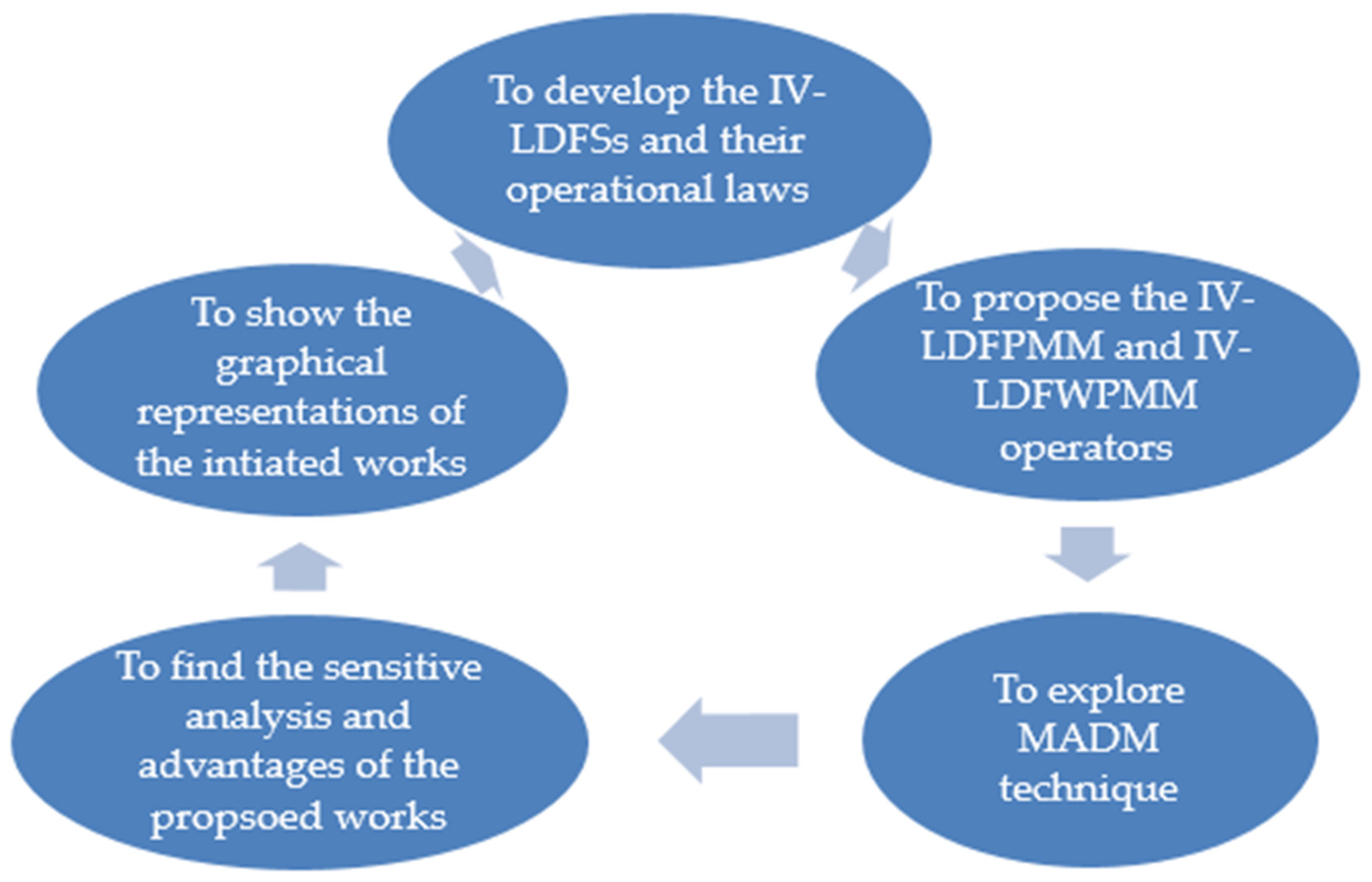
• Analysis of the IV-LDF settings and use of their algebraic laws.
• Introduction of the IV-LDFPMM and IV-LDFWPMM operators, and discussion of some special properties and results.
• Demonstration of the beneficial optimum by using the MADM approach through examples.
• Demonstration of the advantages through a comparative analysis and geometrical interpretations.

The paper is organized as follows: Section 2 gives an overview of IV-QROFS, power aggregation (PA), MM operators, and several related laws. Section 3 analyzes the IV-LDF setting and utilizes their algebraic laws. Section 4 introduces the IV-LDFPMM and IV-LDFWPMM operators and discusses some special properties and results. Section 5 demonstrates the beneficial optimum using the MADM approach and gives examples.

Figure 1 represents the contributions graphically.

2. Preliminaries

This section aims to review the IV-QROFSs, PA, MM operators, and several related laws. The notation used in this analysis is given in

Table 1. Notation used in the present work.

Symbol	Name	Symbol	Name	Symbol	Name
$\mathit{X}$	Universal set	$\psi$	Element of $X$	${\mu }_D$	Truth Grade
${\mathit{\eta }}_{\mathit{D}}\mathbf{\left(}\mathit{\psi }\mathbf{\right)}$	Falsity grade	$a_D$	Reference Parameter for Truth grade	$b_D$	Reference Parameter for Falsity grade
$\mathit{\lambda }\mathbf{\ge }\mathbf{0}$	Scaler element	${\mathsf{\Xi }}_{L_{D1}}$	Accuracy value	${\mathsf{\Pi }}_{L_{D1}}$	Score value

.

Definition 1 [33].

An IV-QROFS$L_D$is defined by:

$$L_D=\left\{\left(\psi ,\left({\mu }_D\left(\psi \right), {\eta }_D\left(\psi \right)\right)\right)/\psi \in X\right\} \left(1\right)$$

(1)

where for MG:${\mu }_D\left(\psi \right)=\left[{\mu }^{-}{ }_D\left(\psi \right),{\mu }^{+}{ }_D\left(\psi \right)\right]\subset \left[0,1\right]$and for NMG:${\eta }_D\left(\psi \right)=\left[{\eta }^{-}{ }_D\left(\psi \right),{\eta }^{+}{ }_D\left(\psi \right)\right]\subset \left[0,1\right]$with the rules of$0\le {\mu }^{+}{ }_D^q\left(\psi \right)+{\eta }^{+}{ }_D^q\left(\psi \right)\le 1,q>0$. The symbol${\chi }_{L_{DFS}}={\left(1-{\mu }^{+}{ }_D^q\left(\psi \right)+{\eta }^{+}{ }_D^q\left(\psi \right)\right)}^{\frac{1}{q}}$expresses the refusal grade. Simply,$L_{D\mathbb{k}}=\left({\mu }_{D\mathbb{k}}, {\eta }_{D\mathbb{k}}\right),\mathbb{k}=1,2,\dots ,\Xi$is called IV-QROFNs.

Definition 2 [33].

For any two IV-QROFNs,$L_{D\mathbb{k}}=\left({\mu }_{D\mathbb{k}}, {\eta }_{D\mathbb{k}}\right)$,$\mathbb{k}=1,2$, and$\lambda \ge 0$:

$$L_{D1}\oplus L_{D2}=\left(\begin{array}{c}\left[{\left({\mu }^{-}{ }_{D1}^q+{\mu }^{-}{ }_{D2}^2-{\mu }^{-}{ }_{D1}^q{\mu }^{-}{ }_{D2}^q\right)}^{\frac{1}{q}},{\left({\mu }^{+}{ }_{D1}^q+{\mu }^{+}{ }_{D2}^q-{\mu }^{+}{ }_{D1}^q{\mu }^{+}{ }_{D2}^q\right)}^{\frac{1}{q}}\right],\\ \left[{\eta }^{-}{ }_{D1}{\eta }^{-}{ }_{D2},{\eta }^{+}{ }_{D1}{\eta }^{+}{ }_{D2}\right]\end{array}\right)$$

(2)

$$L_{D1}\otimes L_{D2}=\left(\begin{array}{c}\left[{\mu }^{-}{ }_{D1}{\mu }^{-}{ }_{D2},{\mu }^{+}{ }_{D1}{\mu }^{+}{ }_{D2}\right],\\ \left[{\left({\eta }^{-}{ }_{D1}^q+{\eta }^{-}{ }_{D2}^q-{\eta }^{-}{ }_{D1}^q{\eta }^{-}{ }_{D2}^q\right)}^{\frac{1}{q}},{\left({\eta }^{+}{ }_{D1}^q+{\eta }^{+}{ }_{D2}^q-{\eta }^{+}{ }_{D1}^q{\eta }^{+}{ }_{D2}^q\right)}^{\frac{1}{q}}\right]\end{array}\right)$$

(3)

$$\lambda L_{D1}=\left(\left[{\left(1-{\left(1-{\mu }^{-}{ }_{D1}^q\right)}^{\lambda }\right)}^{\frac{1}{q}},{\left(1-{\left(1-{\mu }^{+}{ }_{D1}^q\right)}^{\lambda }\right)}^{\frac{1}{q}}\right], \left[{\left({\eta }^{-}{ }_{D1}\right)}^{\lambda },{\left({\eta }^{+}{ }_{D1}\right)}^{\lambda }\right]\right)$$

(4)

$$L_{D1}^{\lambda }=\left(\left[{\left({\mu }^{-}{ }_{D1}\right)}^{\lambda },{\left({\mu }^{+}{ }_{D1}\right)}^{\lambda }\right], \left[{\left(1-{\left(1-{\eta }^{-}{ }_{D1}^q\right)}^{\lambda }\right)}^{\frac{1}{q}},{\left(1-{\left(1-{\eta }^{+}{ }_{D1}^q\right)}^{\lambda }\right)}^{\frac{1}{q}}\right]\right)$$

(5)

Definition 3 [33].

For any IV-QROFN,$L_{D1}=\left({\mu }_{D1}, {\eta }_{D1}\right)$, the Score Value (SV)is defined by:

$${\Xi }_{L_{D1}}=\Xi \left(L_{D1}\right)=\frac{1}{2}\left({\mu }^{+}{ }_{D1}^q+{\mu }^{-}{ }_{D1}^q-{\eta }^{+}{ }_{D1}^q-{\eta }^{-}{ }_{D1}^q\right)$$

(6)

Definition 4 [33].

For any IV-QROFN,$L_{D1}=\left({\mu }_{D1}, {\eta }_{D1}\right)$, the Accuracy Value (AV)is defined by:

$${\mathsf{\Pi }}_{L_{D1}}=\mathsf{\Pi }\left(L_{D1}\right)=\frac{1}{2}\left({\mu }^{+}{ }_{D1}^q+{\mu }^{-}{ }_{D1}^q+{\eta }^{+}{ }_{D1}^q+{\eta }^{-}{ }_{D1}^q\right)$$

(7)

Definition 5 [33].

For any two IV-QROFNs,$L_{D\mathbb{k}}=\left({\mu }_{D\mathbb{k}}, {\eta }_{D\mathbb{k}}\right)$,$\mathbb{k}=1,2$:

1. 

If${\Xi }_{L_{D1}}>{\Xi }_{L_{D2}}$, then$L_{D1}>L_{D2}$;

2. 

If${\Xi }_{L_{D1}}={\Xi }_{L_{D2}}$, then;

(i) 

If${\Pi }_{L_{D1}}>{\Pi }_{L_{D2}}$, then$L_{D1}<L_{D2}$;

(ii) 

If${\Pi }_{L_{D1}}={\Pi }_{L_{D2}}$, then$L_{D1}=L_{D2}$;

Definition 6 [35].

For any collection of non-negative real numbers (CNNRN)$m_{\mathbb{k}}$,$\mathbb{k}=1,2,\dots ,\Xi$, the the PA operator is defined by:

$$PA\left(m_1,m_2,\dots ,m_{\Xi }\right)=\frac{{\sum }_{\mathbb{k}=1}^{\Xi }\left(1+T\left(m_{\mathbb{k}}\right)\right)m_{\mathbb{k}}}{{\sum }_{\mathbb{k}=1}^{\Xi }\left(1+T\left(m_{\mathbb{k}}\right)\right)}$$

(8)

$T\left(m_{\mathbb{k}}\right)=\sum _{j=1, j\ne \mathbb{k}}^{\Xi }sup\left(m_{\mathbb{k}},m_j\right)$and$sup \left(m_{\mathbb{k}},m_j\right)$assigns the support degree from$m_j$to$m_{\mathbb{k}}$, by holding the following conditions:

1. 

$sup\left(m_{\mathbb{k}},m_j\right)\in \left[0,1\right]$;

2. 

$sup\left(m_{\mathbb{k}},m_j\right)=sup\left(m_j,m_{\mathbb{k}}\right)$;

3. 

$sup\left(m_1,m_2\right)\ge sup\left(m_3,m_4\right)$, if$\left|m_1-m_2\right|\le \left|m_3-m_4\right|$.

Definition 7 [35].

For any CNNRN$m_{\mathbb{k}}$,$\mathbb{k}=1,2,\dots ,\Xi$, and a collection of parameters (COP)$\mathsf{{\rm Y}}=\left({\mathsf{{\rm Y}}}_1, {\mathsf{{\rm Y}}}_2,\dots , {\mathsf{{\rm Y}}}_{\Xi }\right)$, where${\mathsf{{\rm Y}}}_{\mathbb{k}},\mathbb{k}=1,2,\dots ,\Xi$is a CNNRN, the Muirhead mean MM Operator is defined by:

$$M{M}^{\mathsf{{\rm Y}}}\left(m_1,m_2,\dots ,m_{\Xi }\right)={\left(\frac{1}{\Xi !}\sum _{𝓅\in T_{\Xi }}\prod _{\mathbb{k}=1}^{\Xi }{m}_{𝓅\left(\mathbb{k}\right)}^{{\mathsf{{\rm Y}}}_{\mathbb{k}}}\right)}^{\frac{1}{{\sum }_{\mathbb{k}=1}^{\Xi }{\mathsf{{\rm Y}}}_{\mathbb{k}}}}$$

(9)

where$𝓅\left(\mathbb{k}\right), \mathbb{k}=1,2,\dots ,\Xi$denotes any permutation of$1,2,\dots ,\Xi$and$T_{\Xi }$shows all feasible permutations of$1,2,\dots ,\Xi$.

3. Interval-Valued Linear Diophantine Fuzzy Sets

It is very beneficial for every company to have a strong decision-making technique at their disposal. Experts and managers involved in decision-making strategies would particularly benefit from such a technique in order to have a crucial impact on the strategy of their company. This section aims to analyze the IV-LDF setting and to use its algebraic laws.

Definition 8. 

An IV-LDFS$L_{DFS}$is defined by:

$$L_{DFS}=\left\{\left(\psi ,\left({\mu }_D\left(\psi \right), {\eta }_D\left(\psi \right)\right), \left(a_D,b_D\right)\right)/\psi \in X\right\}$$

(10)

where${\mu }_D\left(\psi \right)=\left[{\mu }^{-}{ }_D\left(\psi \right),{\mu }^{+}{ }_D\left(\psi \right)\right]\subset \left[0,1\right]$,${\eta }_D\left(\psi \right)=\left[{\eta }^{-}{ }_D\left(\psi \right),{\eta }^{+}{ }_D\left(\psi \right)\right]\subset \left[0,1\right]$,$a_D=\left[a^{-}{ }_D,a^{+}{ }_D\right]\subset \left[0,1\right]$,$b_D=\left[b^{-}{ }_D,{\beta }^{+}{ }_D\right]\subset \left[0,1\right]$, with the rules of$0\le a^{+}{ }_D{\mu }^{+}{ }_D\left(\psi \right)+b^{+}{ }_D{\eta }^{+}{ }_D\left(\psi \right)\le 1$, and$0\le a^{+}{ }_D+b^{+}{ }_D\le 1$. The symbol${\chi }_{L_{DFS}}\sigma {\left(\psi \right)}_{L_{DFS}}=1-\left(a^{+}{ }_D{\mu }^{+}{ }_D\left(\psi \right)+b^{+}{ }_D{\eta }^{+}{ }_D\left(\psi \right)\right)$expresses the refusal grade. Simply$L_{DFS}=\left(\left({\mu }_D, {\eta }_D\right), \left(a_D,b_D\right)\right)$is called IV-LDFN.

Definition 9. 

For any two IV-LDFNs,$L_{D\mathbb{k}}=\left(\left({\mu }_{D\mathbb{k}}, {\eta }_{D\mathbb{k}}\right),\left(a_{D\mathbb{k}}, b_{D\mathbb{k}}\right)\right)$,$\mathbb{k}=1,2$, and$\lambda \ge 0$:

$$L_{D1}\oplus L_{D2}=\left(\begin{array}{c}\left(\begin{array}{c}[{\mu }^{-}{ }_{D1}+{\mu }^{-}{ }_{D2}-{\mu }^{-}{ }_{D1}{\mu }^{-}{ }_{D2},{\mu }^{+}{ }_{D1}+{\mu }^{+}{ }_{D2}-{\mu }^{+}{ }_{D1}{\mu }^{+}{ }_{D2}],\\ \left[{\eta }^{-}{ }_{D1}{\eta }^{-}{ }_{D2},{\eta }^{+}{ }_{D1}{\eta }^{+}{ }_{D2}\right]\end{array}\right),\\ \left(\begin{array}{c}\left[a^{-}{ }_{D1}+a^{-}{ }_{D2}-a^{-}{ }_{D1}{a}^{-}{ }_{D2},a^{+}{ }_{D1}+a^{+}{ }_{D2}-a^{+}{ }_{D1}{a}^{+}{ }_{D2}\right],\\ \left[b^{-}{ }_{D1}{b}^{-}{ }_{D2},b^{+}{ }_{D1}{b}^{+}{ }_{D2}\right]\end{array}\right)\end{array}\right)$$

(11)

$$L_{D1}\otimes L_{D2}=\left(\begin{array}{c}\left(\begin{array}{c}\left[{\mu }^{-}{ }_{D1}{\mu }^{-}{ }_{D2},{\mu }^{+}{ }_{D1}{\mu }^{+}{ }_{D2}\right],\\ \left[{\eta }^{-}{ }_{D1}+{\eta }^{-}{ }_{D2}-{\eta }^{-}{ }_{D1}{\eta }^{-}{ }_{D2},{\eta }^{+}{ }_{D1}+{\eta }^{+}{ }_{D2}-{\eta }^{+}{ }_{D1}{\eta }^{+}{ }_{D2}\right]\end{array}\right),\\ \left(\begin{array}{c}\left[a^{-}{ }_{D1}{a}^{-}{ }_{D2},a^{+}{ }_{D1}{a}^{+}{ }_{D2}\right]\\ \left[b^{-}{ }_{D1}+b^{-}{ }_{D2}-b^{-}{ }_{D1}{b}^{-}{ }_{D2},b^{+}{ }_{D1}+b^{+}{ }_{D2}-b^{+}{ }_{D1}{b}^{+}{ }_{D2}\right],\end{array}\right)\end{array}\right)$$

(12)

$$\lambda L_{D1}=\left(\begin{array}{c}\left(\begin{array}{c}\left[1-{\left(1-{\mu }^{-}{ }_{D1}\right)}^{\lambda },1-{\left(1-{\mu }^{+}{ }_{D1}\right)}^{\lambda }\right],\\ \left[{\left({\eta }^{-}{ }_{D1}\right)}^{\lambda },{\left({\eta }^{+}{ }_{D1}\right)}^{\lambda }\right]\end{array}\right),\\ \left(\begin{array}{c}\left[1-{\left(1-a^{-}{ }_{D1}\right)}^{\lambda },1-{\left(1-a^{+}{ }_{D1}\right)}^{\lambda }\right], \\ \left[{\left(b^{-}{ }_{D1}\right)}^{\lambda },{\left(b^{+}{ }_{D1}\right)}^{\lambda }\right]\end{array}\right)\end{array}\right)$$

(13)

$$L_{D1}^{\lambda }=\left(\begin{array}{c}\left(\begin{array}{c}\left[{\left({\mu }^{-}{ }_{D1}\right)}^{\lambda },{\left({\mu }^{+}{ }_{D1}\right)}^{\lambda }\right],\\ \left[1-{\left(1-{\eta }^{-}{ }_{D1}\right)}^{\lambda },1-{\left(1-{\eta }^{+}{ }_{D1}\right)}^{\lambda }\right]\end{array}\right),\\ \left(\left[{\left(a^{-}{ }_{D1}\right)}^{\lambda },{\left(a^{+}{ }_{D1}\right)}^{\lambda }\right], \left[1-{\left(1-b^{-}{ }_{D1}\right)}^{\lambda },1-{\left(1-b^{+}{ }_{D1}\right)}^{\lambda }\right]\right)\end{array}\right)$$

(14)

Definition 10. 

For any IV-LDFN,$L_{D1}=\left(\left({\mu }_{D1}, {\eta }_{D1}\right),\left(a_{D1}, b_{D1}\right)\right)$, the SVis defined by:

$${\Xi }_{L_{D1}}=\Xi \left(L_{D1}\right)=\frac{1}{2}\left(\begin{array}{c}{a}^{+}{ }_{D1}{\mu }^{+}{ }_{D1}-b^{+}{ }_{D1}{\eta }^{+}{ }_{D1}+\\ a^{-}{ }_{D1}{\mu }^{-}{ }_{D1}-b^{-}{ }_{D1}{\eta }^{-}{ }_{D1}\end{array}\right)$$

(15)

Definition 11. 

For any IV-LDFN,$L_{D1}=\left(\left({\mu }_{D1}, {\eta }_{D1}\right),\left(a_{D1}, b_{D1}\right)\right)$, the AVis defined by:

$${\mathsf{\Pi }}_{L_{D1}}=\mathsf{\Pi }\left(L_{D1}\right)=\frac{1}{2}\left(\begin{array}{c}{a}^{+}{ }_{D1}{\mu }^{+}{ }_{D1}+b^{+}{ }_{D1}{\eta }^{+}{ }_{D1}+\\ a^{-}{ }_{D1}{\mu }^{-}{ }_{D1}+b^{-}{ }_{D1}{\eta }^{-}{ }_{D1}\end{array}\right)$$

(16)

Definition 12.  

For any two IV-LDFNs,$L_{D\mathbb{k}}=\left(\left({\mu }_{D\mathbb{k}}, {\eta }_{D\mathbb{k}}\right),\left(a_{D\mathbb{k}}, b_{D\mathbb{k}}\right)\right)$,$\mathbb{k}=1,2$:

1. 

If${\Xi }_{L_{D1}}>{\Xi }_{L_{D2}}$, then$L_{D1}>L_{D2}$;

2. 

If${\Xi }_{L_{D1}}={\Xi }_{L_{D2}}$, then;

(i) 

If${\Pi }_{L_{D1}}>{\Pi }_{L_{D2}}$, then$L_{D1}<L_{D2}$;

(ii) 

If${\Pi }_{L_{D1}}={\Pi }_{L_{D2}}$, then$L_{D1}=L_{D2}$;

4. Power Muirhead Mean (MM) Operators under the IV-LDFSs

Starting from the MM operator and IV-LDF data, the IV-LDFPMM and the IV-LDFWPMM operators are introduced, and some special properties and results are to be shown. Furthermore, for any collection of IV-LDFNs, $L_{D\mathbb{k}}=\left(\left({\mu }_{D\mathbb{k}}, {\eta }_{D\mathbb{k}}\right),\left(a_{D\mathbb{k}}, b_{D\mathbb{k}}\right)\right)$, $\mathbb{k}=1,2,\dots ,\Xi$ and let $\mathsf{{\rm Y}}=\left({\mathsf{{\rm Y}}}_1,{ \mathsf{{\rm Y}}}_2,\dots ,{ \mathsf{{\rm Y}}}_{\Xi }\right)$ be a COP, where ${\mathsf{{\rm Y}}}_{\mathbb{k}},\mathbb{k}=1,2,\dots ,\Xi$ is a CNNRN. The vector $𝓌={\left({𝓌}_1,{𝓌}_2,\dots ,{𝓌}_{\Xi }\right)}^T$ is the weight vector whereby: $\sum _{\mathbb{k}=1}^{\Xi }{𝓌}_{\mathbb{k}}=1$ and ${𝓌}_{\mathbb{k}}\in \left[0,1\right], \mathbb{k}=1,2,\dots ,\Xi$.

Definition 13. 

The IV-LDFPMM Operator is defined by:

$$\mathrm{IV}-{\mathrm{LDFPMM}}^{\mathsf{{\rm Y}}}\left(L_{D1},L_{D2},\dots ,L_{D\mathbb{k}}\right)={\left(\frac{1}{\Xi !}\begin{array}{c}\oplus \\ 𝓅\in T_{\Xi }\end{array}\begin{array}{c}\Xi \\ \otimes \\ \mathbb{k}\end{array} {\left(\Xi \frac{\left(1+T\left(L_{𝓅\left(\mathbb{k}\right)}\right)\right)}{{\sum }_{\mathbb{k}=1}^{\Xi }\left(1+T\left(𝓅\left(\mathbb{k}\right)\right)\right)}{L}_{𝓅\left(\mathbb{k}\right)}\right)}^{{\mathsf{{\rm Y}}}_{\mathbb{k}}}\right)}^{\frac{1}{{\sum }_{\mathbb{k}=1}^{\Xi }{\mathsf{{\rm Y}}}_{\mathbb{k}}}}$$

(17)

where$𝓅\left(\mathbb{k}\right), \mathbb{k}=1,2,\dots ,\Xi$denotes any permutation of$1,2,\dots ,\Xi$and$T_{\Xi }$includes all feasible permutations of$1,2,\dots ,\Xi$, and$\Xi$is the weighting measurement.$\mathrm{𝕕} \left(L_{D\mathbb{k}},L_{Dj}\right)=\frac{1}{2}\left(\begin{array}{c}{a}^{+}{ }_{D1}{\mu }^{+}{ }_{D1}-b^{+}{ }_{D1}{\eta }^{+}{ }_{D1}+\\ a^{-}{ }_{D1}{\mu }^{-}{ }_{D1}-b^{-}{ }_{D1}{\eta }^{-}{ }_{D1}\end{array}\right)$, shows the Hamming distance between$L_{D\mathbb{k}}$and$L_{Dj}$,$sup\left(L_{D\mathbb{k}},L_{Dj}\right)$denotes the support degree from$L_{Dj}$to$L_{D\mathbb{k}}$, holding the following conditions:

1.  

$sup\left(L_{D\mathbb{k}},L_{Dj}\right)\in \left[0,1\right]$;

2.  

$sup\left(L_{D\mathbb{k}},L_{Dj}\right)=sup\left(L_{Dj},L_{D\mathbb{k}}\right)$;

3. 

$sup\left(L_{D1},L_{D2}\right)\ge sup\left(L_{D3},L_{D4}\right)$, if$\left|L_{D1}-L_{D2}\right|\le \left|L_{D3}-L_{D4}\right|$.

To simplify Equation (17), one may introduce

$${𝓌}_{\mathbb{k}}=\frac{\left(1+T\left(L_{D\mathbb{k}}\right)\right)}{{\sum }_{\mathbb{k}}^{\Xi }\left(1+T\left(L_{D\mathbb{k}}\right)\right)}$$

(18)

Then, Equation (17) can be written as:

$$\mathrm{IV}-{\mathrm{LDFPMM}}^{\mathsf{{\rm Y}}}\left(L_{D1},L_{D2},\dots ,L_{D\mathbb{k}}\right)={\left(\frac{1}{\Xi !}\begin{array}{c}\oplus \\ 𝓅\in T_{\Xi }\end{array}\begin{array}{c}\Xi \\ \otimes \\ \mathbb{k}\end{array} {\left(\Xi {𝓌}_{𝓅\left(\mathbb{k}\right)}{L}_{𝓅\left(\mathbb{k}\right)}\right)}^{{\mathsf{{\rm Y}}}_{\mathbb{k}}}\right)}^{\frac{1}{{\sum }_{\mathbb{k}=1}^{\Xi }{\mathsf{{\rm Y}}}_{\mathbb{k}}}}$$

(19)

Based on Equations (17)–(19), the following theorems can be proven.

Theorem 1. 

Based on Equations (17)–(19), we obtain:

$$\mathrm{IV}-{\mathrm{LDFPMM}}^{\mathsf{{\rm Y}}}\left(L_{D1},L_{D2},\dots ,L_{D\mathbb{k}}\right)=\left(\begin{array}{c}\left(\begin{array}{c}\left[\begin{array}{c}{\left(1-{\left({\displaystyle \prod _{𝓅\in T_{\Xi }}^{\Xi }}\left(1-\left({\displaystyle \prod _{\mathbb{k}=1}^{\Xi }}{\left(1-{\left(1-{\mu }_{𝓅\left(\mathbb{k}\right)}^{-}\right)}^{\Xi {𝓌}_{𝓅\left(\mathbb{k}\right)}}\right)}^{{\mathsf{{\rm Y}}}_{\mathbb{k}}}\right)\right)\right)}^{\frac{1}{\Xi !}}\right)}^{\frac{1}{{\sum }_{\mathbb{k}=1}^{\Xi }{\mathsf{{\rm Y}}}_{\mathbb{k}}}},\\ {\left(1-{\left({\displaystyle \prod _{𝓅\in T_{\Xi }}^{\Xi }}\left(1-\left({\displaystyle \prod _{\mathbb{k}=1}^{\Xi }}{\left(1-{\left(1-{\mu }_{𝓅\left(\mathbb{k}\right)}^{+}\right)}^{\Xi {𝓌}_{𝓅\left(\mathbb{k}\right)}}\right)}^{{\mathsf{{\rm Y}}}_{\mathbb{k}}}\right)\right)\right)}^{\frac{1}{\Xi !}}\right)}^{\frac{1}{{\sum }_{\mathbb{k}=1}^{\Xi }{\mathsf{{\rm Y}}}_{\mathbb{k}}}}\end{array}\right],\\ \left[\begin{array}{c}1-{\left(1-{\left({\displaystyle \prod _{𝓅\in T_{\Xi }}^{\Xi }}\left(1-{\displaystyle \prod _{\mathbb{k}=1}^{\Xi }}{\left(1-{\eta }_{𝓅\left(\mathbb{k}\right)}^{-}{}^{\Xi {𝓌}_{𝓅\left(\mathbb{k}\right)}}\right)}^{{\mathsf{{\rm Y}}}_{\mathbb{k}}}\right)\right)}^{\frac{1}{\Xi !}}\right)}^{\frac{1}{{\sum }_{\mathbb{k}=1}^{\Xi }{\mathsf{{\rm Y}}}_{\mathbb{k}}}},\\ 1-{\left(1-{\left({\displaystyle \prod _{𝓅\in T_{\Xi }}^{\Xi }}\left(1-{\displaystyle \prod _{\mathbb{k}=1}^{\Xi }}{\left(1-{\eta }_{𝓅\left(\mathbb{k}\right)}^{+}{}^{\Xi {𝓌}_{𝓅\left(\mathbb{k}\right)}}\right)}^{{\mathsf{{\rm Y}}}_{\mathbb{k}}}\right)\right)}^{\frac{1}{\Xi !}}\right)}^{\frac{1}{{\sum }_{\mathbb{k}=1}^{\Xi }{\mathsf{{\rm Y}}}_{\mathbb{k}}}}\end{array}\right]\end{array}\right),\\ \left[\begin{array}{c}{\left(1-{\left({\displaystyle \prod _{𝓅\in T_{\Xi }}^{\Xi }}\left(1-\left({\displaystyle \prod _{\mathbb{k}=1}^{\Xi }}{\left(1-{\left(1-a_{𝓅\left(\mathbb{k}\right)}^{-}\right)}^{\Xi {𝓌}_{𝓅\left(\mathbb{k}\right)}}\right)}^{{\mathsf{{\rm Y}}}_{\mathbb{k}}}\right)\right)\right)}^{\frac{1}{\Xi !}}\right)}^{\frac{1}{{\sum }_{\mathbb{k}=1}^{\Xi }{\mathsf{{\rm Y}}}_{\mathbb{k}}}},\\ {\left(1-{\left({\displaystyle \prod _{𝓅\in T_{\Xi }}^{\Xi }}\left(1-\left({\displaystyle \prod _{\mathbb{k}=1}^{\Xi }}{\left(1-{\left(1-a_{𝓅\left(\mathbb{k}\right)}^{+}\right)}^{\Xi {𝓌}_{𝓅\left(\mathbb{k}\right)}}\right)}^{{\mathsf{{\rm Y}}}_{\mathbb{k}}}\right)\right)\right)}^{\frac{1}{\Xi !}}\right)}^{\frac{1}{{\sum }_{\mathbb{k}=1}^{\Xi }{\mathsf{{\rm Y}}}_{\mathbb{k}}}}\end{array}\right],\\ \left[\begin{array}{c}1-{\left(1-{\left({\displaystyle \prod _{𝓅\in T_{\Xi }}^{\Xi }}\left(1-{\displaystyle \prod _{\mathbb{k}=1}^{\Xi }}{\left(1-b_{𝓅\left(\mathbb{k}\right)}^{-}{}^{\Xi {𝓌}_{𝓅\left(\mathbb{k}\right)}}\right)}^{{\mathsf{{\rm Y}}}_{\mathbb{k}}}\right)\right)}^{\frac{1}{\Xi !}}\right)}^{\frac{1}{{\sum }_{\mathbb{k}=1}^{\Xi }{\mathsf{{\rm Y}}}_{\mathbb{k}}}},\\ 1-{\left(1-{\left({\displaystyle \prod _{𝓅\in T_{\Xi }}^{\Xi }}\left(1-{\displaystyle \prod _{\mathbb{k}=1}^{\Xi }}{\left(1-b_{𝓅\left(\mathbb{k}\right)}^{+}{}^{\Xi {𝓌}_{𝓅\left(\mathbb{k}\right)}}\right)}^{{\mathsf{{\rm Y}}}_{\mathbb{k}}}\right)\right)}^{\frac{1}{\Xi !}}\right)}^{\frac{1}{{\sum }_{\mathbb{k}=1}^{\Xi }{\mathsf{{\rm Y}}}_{\mathbb{k}}}}\end{array}\right]\end{array}\right)$$

(20)

Proof. 

Based on Definition 9 and Equation (20), we obtain:

$$\Xi {𝓌}_{𝓅\left(\mathbb{k}\right)}{L}_{𝓅\left(\mathbb{k}\right)}=\left(\begin{array}{c}\left(\left[1-{\left(1-{\mu }_{𝓅\left(\mathbb{k}\right)}^{-}\right)}^{\Xi {𝓌}_{𝓅\left(\mathbb{k}\right)}},1-{\left(1-{\mu }_{𝓅\left(\mathbb{k}\right)}^{+}\right)}^{\Xi {𝓌}_{𝓅\left(\mathbb{k}\right)}}\right],\left[{\eta }_{𝓅\left(\mathbb{k}\right)}^{-}{}^{\Xi {𝓌}_{𝓅\left(\mathbb{k}\right)}},{\eta }_{𝓅\left(\mathbb{k}\right)}^{+}{}^{\Xi {𝓌}_{𝓅\left(\mathbb{k}\right)}}\right]\right),\\ \left(\left[1-{\left(1-a_{𝓅\left(\mathbb{k}\right)}^{-}\right)}^{\Xi {𝓌}_{𝓅\left(\mathbb{k}\right)}},1-{\left(1-a_{𝓅\left(\mathbb{k}\right)}^{+}\right)}^{\Xi {𝓌}_{𝓅\left(\mathbb{k}\right)}}\right],\left[b_{𝓅\left(\mathbb{k}\right)}^{-}{}^{\Xi {𝓌}_{𝓅\left(\mathbb{k}\right)}},b_{𝓅\left(\mathbb{k}\right)}^{+}{}^{\Xi {𝓌}_{𝓅\left(\mathbb{k}\right)}}\right]\right)\end{array}\right)$$

and

$${\left(\Xi {𝓌}_{𝓅\left(\mathbb{k}\right)}{L}_{𝓅\left(\mathbb{k}\right)}\right)}^{{\mathsf{{\rm Y}}}_{\mathbb{k}}}=\left(\begin{array}{c}\left(\right[{\left(1-{\left(1-{\mu }_{𝓅\left(\mathbb{k}\right)}^{-}\right)}^{\Xi {𝓌}_{𝓅\left(\mathbb{k}\right)}}\right)}^{\mathsf{{\rm Y}}\mathbb{k}},{(1-{\left(1-{\mu }_{𝓅\left(\mathbb{k}\right)}^{+}\right)}^{\Xi {𝓌}_{𝓅\left(\mathbb{k}\right)}}}^{\mathsf{{\rm Y}}\mathbb{k}}],[1-{(1-{{𝜂}_{𝓅\left(\mathbb{k}\right)}^{-}}^{\Xi {𝓌}_{𝓅\left(\mathbb{k}\right)}})}^{\mathsf{{\rm Y}}\mathbb{k}},1-{(1-{{𝜂}_{𝓅\left(\mathbb{k}\right)}^{+}}^{\Xi {𝓌}_{𝓅\left(\mathbb{k}\right)}})}^{\mathsf{{\rm Y}}\mathbb{k}}\left]\right),\\ \left(\right[{\left(1-{\left(1-a_{𝓅\left(\mathbb{k}\right)}^{-}\right)}^{\Xi {𝓌}_{𝓅\left(\mathbb{k}\right)}}\right)}^{\mathsf{{\rm Y}}\mathbb{k}},{(1-{\left(1-a_{𝓅\left(\mathbb{k}\right)}^{+}\right)}^{\Xi {𝓌}_{𝓅\left(\mathbb{k}\right)}}}^{\mathsf{{\rm Y}}\mathbb{k}}],[1-{(1-{b_{𝓅\left(\mathbb{k}\right)}^{-}}^{\Xi {𝓌}_{𝓅\left(\mathbb{k}\right)}})}^{\mathsf{{\rm Y}}\mathbb{k}},1-{(1-{b_{𝓅\left(\mathbb{k}\right)}^{+}}^{\Xi {𝓌}_{𝓅\left(\mathbb{k}\right)}})}^{\mathsf{{\rm Y}}\mathbb{k}}\left]\right),\end{array}\right)$$

Furthermore,

$$\begin{array}{c}\Xi \\ \oplus \\ \mathbb{k}\end{array}{\left(\Xi {𝓌}_{𝓅\left(\mathbb{k}\right)}{L}_{𝓅\left(\mathbb{k}\right)}\right)}^{{\mathsf{{\rm Y}}}_{\mathbb{k}}}=\left(\begin{array}{c}\left(\begin{array}{c}\left[{\displaystyle \prod _{\mathbb{k}=1}^{\Xi }}{\left(1-{\left(1-{\mu }_{𝓅\left(\mathbb{k}\right)}^{-}\right)}^{\Xi {𝓌}_{𝓅\left(\mathbb{k}\right)}}\right)}^{{\mathsf{{\rm Y}}}_{\mathbb{k}}},{\displaystyle \prod _{\mathbb{k}=1}^{\Xi }}{\left(1-{\left(1-{\mu }_{𝓅\left(\mathbb{k}\right)}^{+}\right)}^{\Xi {𝓌}_{𝓅\left(\mathbb{k}\right)}}\right)}^{{\mathsf{{\rm Y}}}_{\mathbb{k}}}\right],\\ \left[1-{\displaystyle \prod _{\mathbb{k}=1}^{\Xi }}{\left(1-{\eta }_{𝓅\left(\mathbb{k}\right)}^{-}{}^{\Xi {𝓌}_{𝓅\left(\mathbb{k}\right)}}\right)}^{{\mathsf{{\rm Y}}}_{\mathbb{k}}},1-{\displaystyle \prod _{\mathbb{k}=1}^{\Xi }}{\left(1-{\eta }_{𝓅\left(\mathbb{k}\right)}^{+}{}^{\Xi {𝓌}_{𝓅\left(\mathbb{k}\right)}}\right)}^{{\mathsf{{\rm Y}}}_{\mathbb{k}}}\right]\end{array}\right),\\ \left(\begin{array}{c}\left[{\displaystyle \prod _{\mathbb{k}=1}^{\Xi }}{\left(1-{\left(1-a_{𝓅\left(\mathbb{k}\right)}^{-}\right)}^{\Xi {𝓌}_{𝓅\left(\mathbb{k}\right)}}\right)}^{{\mathsf{{\rm Y}}}_{\mathbb{k}}},{\displaystyle \prod _{\mathbb{k}=1}^{\Xi }}{\left(1-{\left(1-a_{𝓅\left(\mathbb{k}\right)}^{+}\right)}^{\Xi {𝓌}_{𝓅\left(\mathbb{k}\right)}}\right)}^{{\mathsf{{\rm Y}}}_{\mathbb{k}}}\right],\\ \left[1-{\displaystyle \prod _{\mathbb{k}=1}^{\Xi }}{\left(1-b_{𝓅\left(\mathbb{k}\right)}^{-}{}^{\Xi {𝓌}_{𝓅\left(\mathbb{k}\right)}}\right)}^{{\mathsf{{\rm Y}}}_{\mathbb{k}}},1-{\displaystyle \prod _{\mathbb{k}=1}^{\Xi }}{\left(1-b_{𝓅\left(\mathbb{k}\right)}^{+}{}^{\Xi {𝓌}_{𝓅\left(\mathbb{k}\right)}}\right)}^{{\mathsf{{\rm Y}}}_{\mathbb{k}}}\right]\end{array}\right)\end{array}\right)$$

Also,

$$\begin{array}{c}\oplus \\ 𝓅\in T_{\Xi }\end{array}\begin{array}{c}\Xi \\ \otimes \\ \mathbb{k}\end{array} {\left(\Xi {𝓌}_{𝓅\left(\mathbb{k}\right)}{L}_{𝓅\left(\mathbb{k}\right)}\right)}^{{\mathsf{{\rm Y}}}_{\mathbb{k}}}=\left(\begin{array}{c}\left(\begin{array}{c}\left[1-{\displaystyle \prod _{𝓅\in T_{\Xi }}^{\Xi }}\left(1-\left({\displaystyle \prod _{\mathbb{k}=1}^{\Xi }}{\left(1-{\left(1-{\mu }_{𝓅\left(\mathbb{k}\right)}^{-}\right)}^{\Xi {𝓌}_{𝓅\left(\mathbb{k}\right)}}\right)}^{{\mathsf{{\rm Y}}}_{\mathbb{k}}}\right)\right),1-{\displaystyle \prod _{𝓅\in T_{\Xi }}^{\Xi }}\left(1-\left({\displaystyle \prod _{\mathbb{k}=1}^{\Xi }}{\left(1-{\left(1-{\mu }_{𝓅\left(\mathbb{k}\right)}^{+}\right)}^{\Xi {𝓌}_{𝓅\left(\mathbb{k}\right)}}\right)}^{{\mathsf{{\rm Y}}}_{\mathbb{k}}}\right)\right)\right],\\ \left[{\displaystyle \prod _{𝓅\in T_{\Xi }}^{\Xi }}\left(1-{\displaystyle \prod _{\mathbb{k}=1}^{\Xi }}{\left(1-{\eta }_{𝓅\left(\mathbb{k}\right)}^{-}{}^{\Xi {𝓌}_{𝓅\left(\mathbb{k}\right)}}\right)}^{{\mathsf{{\rm Y}}}_{\mathbb{k}}}\right),{\displaystyle \prod _{𝓅\in T_{\Xi }}^{\Xi }}\left(1-{\displaystyle \prod _{\mathbb{k}=1}^{\Xi }}{\left(1-{\eta }_{𝓅\left(\mathbb{k}\right)}^{+}{}^{\Xi {𝓌}_{𝓅\left(\mathbb{k}\right)}}\right)}^{{\mathsf{{\rm Y}}}_{\mathbb{k}}}\right)\right]\end{array}\right),\\ \left(\begin{array}{c}\left[1-{\displaystyle \prod _{𝓅\in T_{\Xi }}^{\Xi }}\left(1-\left({\displaystyle \prod _{\mathbb{k}=1}^{\Xi }}{\left(1-{\left(1-a_{𝓅\left(\mathbb{k}\right)}^{-}\right)}^{\Xi {𝓌}_{𝓅\left(\mathbb{k}\right)}}\right)}^{{\mathsf{{\rm Y}}}_{\mathbb{k}}}\right)\right),1-{\displaystyle \prod _{𝓅\in T_{\Xi }}^{\Xi }}\left(1-\left({\displaystyle \prod _{\mathbb{k}=1}^{\Xi }}{\left(1-{\left(1-a_{𝓅\left(\mathbb{k}\right)}^{+}\right)}^{\Xi {𝓌}_{𝓅\left(\mathbb{k}\right)}}\right)}^{{\mathsf{{\rm Y}}}_{\mathbb{k}}}\right)\right)\right],\\ \left[{\displaystyle \prod _{𝓅\in T_{\Xi }}^{\Xi }}\left(1-{\displaystyle \prod _{\mathbb{k}=1}^{\Xi }}{\left(1-b_{𝓅\left(\mathbb{k}\right)}^{-}{}^{\Xi {𝓌}_{𝓅\left(\mathbb{k}\right)}}\right)}^{{\mathsf{{\rm Y}}}_{\mathbb{k}}}\right),{\displaystyle \prod _{𝓅\in T_{\Xi }}^{\Xi }}\left(1-{\displaystyle \prod _{\mathbb{k}=1}^{\Xi }}{\left(1-b_{𝓅\left(\mathbb{k}\right)}^{+}{}^{\Xi {𝓌}_{𝓅\left(\mathbb{k}\right)}}\right)}^{{\mathsf{{\rm Y}}}_{\mathbb{k}}}\right)\right]\end{array}\right)\end{array}\right)$$

Finally,

$$\frac{1}{\Xi !}\begin{array}{c}\oplus \\ 𝓅\in T_{\Xi }\end{array}\begin{array}{c}\Xi \\ \otimes \\ \mathbb{k}\end{array} {\left(\Xi {𝓌}_{𝓅\left(\mathbb{k}\right)}{L}_{𝓅\left(\mathbb{k}\right)}\right)}^{{\mathsf{{\rm Y}}}_{\mathbb{k}}}=\left(\begin{array}{c}{\left(\begin{array}{c}\left[\begin{array}{c}1-{\left({\displaystyle \prod _{𝓅\in T_{\Xi }}^{\Xi }}\left(1-\left({\displaystyle \prod _{\mathbb{k}=1}^{\Xi }}{\left(1-{\left(1-{\mu }_{𝓅\left(\mathbb{k}\right)}^{-}\right)}^{\Xi {𝓌}_{𝓅\left(\mathbb{k}\right)}}\right)}^{{\mathsf{{\rm Y}}}_{\mathbb{k}}}\right)\right)\right)}^{\frac{1}{\Xi !}},\\ 1-{\left({\displaystyle \prod _{𝓅\in T_{\Xi }}^{\Xi }}\left(1-\left({\displaystyle \prod _{\mathbb{k}=1}^{\Xi }}{\left(1-{\left(1-{\mu }_{𝓅\left(\mathbb{k}\right)}^{+}\right)}^{\Xi {𝓌}_{𝓅\left(\mathbb{k}\right)}}\right)}^{{\mathsf{{\rm Y}}}_{\mathbb{k}}}\right)\right)\right)}^{\frac{1}{\Xi !}}\end{array}\right],\\ \left[{\left({\displaystyle \prod _{𝓅\in T_{\Xi }}^{\Xi }}\left(1-{\displaystyle \prod _{\mathbb{k}=1}^{\Xi }}{\left(1-{\eta }_{𝓅\left(\mathbb{k}\right)}^{-}{}^{\Xi {𝓌}_{𝓅\left(\mathbb{k}\right)}}\right)}^{{\mathsf{{\rm Y}}}_{\mathbb{k}}}\right)\right)}^{\frac{1}{\Xi !}},{\left({\displaystyle \prod _{𝓅\in T_{\Xi }}^{\Xi }}\left(1-{\displaystyle \prod _{\mathbb{k}=1}^{\Xi }}{\left(1-{\eta }_{𝓅\left(\mathbb{k}\right)}^{+}{}^{\Xi {𝓌}_{𝓅\left(\mathbb{k}\right)}}\right)}^{{\mathsf{{\rm Y}}}_{\mathbb{k}}}\right)\right)}^{\frac{1}{\Xi !}}\right]\end{array}\right)}^{,}\\ \left(\begin{array}{c}\left[\begin{array}{c}1-{\left({\displaystyle \prod _{𝓅\in T_{\Xi }}^{\Xi }}\left(1-\left({\displaystyle \prod _{\mathbb{k}=1}^{\Xi }}{\left(1-{\left(1-a_{𝓅\left(\mathbb{k}\right)}^{-}\right)}^{\Xi {𝓌}_{𝓅\left(\mathbb{k}\right)}}\right)}^{{\mathsf{{\rm Y}}}_{\mathbb{k}}}\right)\right)\right)}^{\frac{1}{\Xi !}},\\ 1-{\left({\displaystyle \prod _{𝓅\in T_{\Xi }}^{\Xi }}\left(1-\left({\displaystyle \prod _{\mathbb{k}=1}^{\Xi }}{\left(1-{\left(1-a_{𝓅\left(\mathbb{k}\right)}^{+}\right)}^{\Xi {𝓌}_{𝓅\left(\mathbb{k}\right)}}\right)}^{{\mathsf{{\rm Y}}}_{\mathbb{k}}}\right)\right)\right)}^{\frac{1}{\Xi !}}\end{array}\right],\\ \left[{\left({\displaystyle \prod _{𝓅\in T_{\Xi }}^{\Xi }}\left(1-{\displaystyle \prod _{\mathbb{k}=1}^{\Xi }}{\left(1-b_{𝓅\left(\mathbb{k}\right)}^{-}{}^{\Xi {𝓅}_{𝓌\left(\mathbb{k}\right)}}\right)}^{{\mathsf{{\rm Y}}}_{\mathbb{k}}}\right)\right)}^{\frac{1}{\Xi !}},{\left({\displaystyle \prod _{𝓅\in T_{\Xi }}^{\Xi }}\left(1-{\displaystyle \prod _{\mathbb{k}=1}^{\Xi }}{\left(1-b_{𝓅\left(\mathbb{k}\right)}^{+}{}^{\Xi {𝓌}_{𝓅\left(\mathbb{k}\right)}}\right)}^{{\mathsf{{\rm Y}}}_{\mathbb{k}}}\right)\right)}^{\frac{1}{\Xi !}}\right]\end{array}\right)\end{array}\right)$$

Thus,

$${(\frac{1}{\Xi !}\begin{array}{c}\oplus \\ 𝓅\in T_{\Xi }\end{array}\begin{array}{c}\Xi \\ \otimes \\ \mathbb{k}\end{array} {\left(\Xi {𝓌}_{𝓅\left(\mathbb{k}\right)}{L}_{𝓅\left(\mathbb{k}\right)}\right)}^{{\mathsf{{\rm Y}}}_{\mathbb{k}}})}^{\frac{1}{{\sum }_{\mathbb{k}=1}^{\Xi }{\mathsf{{\rm Y}}}_{\mathbb{k}}}} =\left(\begin{array}{c}\left(\begin{array}{c}\left[\begin{array}{c}{\left(1-{\left({\displaystyle \prod _{𝓅\in T_{\Xi }}^{\Xi }}\left(1-\left({\displaystyle \prod _{\mathbb{k}=1}^{\Xi }}{\left(1-{\left(1-{\mu }_{𝓅\left(\mathbb{k}\right)}^{-}\right)}^{\Xi {𝓌}_{𝓅\left(\mathbb{k}\right)}}\right)}^{{\mathsf{{\rm Y}}}_{\mathbb{k}}}\right)\right)\right)}^{\frac{1}{\Xi !}}\right)}^{\frac{1}{{\sum }_{\mathbb{k}=1}^{\Xi }{\mathsf{{\rm Y}}}_{\mathbb{k}}}},\\ {\left(1-{\left({\displaystyle \prod _{𝓅\in T_{\Xi }}^{\Xi }}\left(1-\left({\displaystyle \prod _{\mathbb{k}=1}^{\Xi }}{\left(1-{\left(1-{\mu }_{𝓅\left(\mathbb{k}\right)}^{+}\right)}^{\Xi {𝓌}_{𝓅\left(\mathbb{k}\right)}}\right)}^{{\mathsf{{\rm Y}}}_{\mathbb{k}}}\right)\right)\right)}^{\frac{1}{\Xi !}}\right)}^{\frac{1}{{\sum }_{\mathbb{k}=1}^{\Xi }{\mathsf{{\rm Y}}}_{\mathbb{k}}}}\end{array}\right],\\ \left[\begin{array}{c}1-{\left(1-{\left({\displaystyle \prod _{𝓅\in T_{\Xi }}^{\Xi }}\left(1-{\displaystyle \prod _{\mathbb{k}=1}^{\Xi }}{\left(1-{\eta }_{𝓅\left(\mathbb{k}\right)}^{-}{}^{\Xi {𝓌}_{𝓅\left(\mathbb{k}\right)}}\right)}^{{\mathsf{{\rm Y}}}_{\mathbb{k}}}\right)\right)}^{\frac{1}{\Xi !}}\right)}^{\frac{1}{{\sum }_{\mathbb{k}=1}^{\Xi }{\mathsf{{\rm Y}}}_{\mathbb{k}}}},\\ 1-{\left(1-{\left({\displaystyle \prod _{𝓅\in T_{\Xi }}^{\Xi }}\left(1-{\displaystyle \prod _{\mathbb{k}=1}^{\Xi }}{\left(1-{\eta }_{𝓅\left(\mathbb{k}\right)}^{+}{}^{\Xi {𝓌}_{𝓅\left(\mathbb{k}\right)}}\right)}^{{\mathsf{{\rm Y}}}_{\mathbb{k}}}\right)\right)}^{\frac{1}{\Xi !}}\right)}^{\frac{1}{{\sum }_{\mathbb{k}=1}^{\Xi }{\mathsf{{\rm Y}}}_{\mathbb{k}}}}\end{array}\right]\end{array}\right),\\ \left[\begin{array}{c}{\left(1-{\left({\displaystyle \prod _{𝓅\in T_{\Xi }}^{\Xi }}\left(1-\left({\displaystyle \prod _{\mathbb{k}=1}^{\Xi }}{\left(1-{\left(1-a_{𝓅\left(\mathbb{k}\right)}^{-}\right)}^{\Xi {𝓌}_{𝓅\left(\mathbb{k}\right)}}\right)}^{{\mathsf{{\rm Y}}}_{\mathbb{k}}}\right)\right)\right)}^{\frac{1}{\Xi !}}\right)}^{\frac{1}{{\sum }_{\mathbb{k}=1}^{\Xi }{\mathsf{{\rm Y}}}_{\mathbb{k}}}},\\ {\left(1-{\left({\displaystyle \prod _{𝓅\in T_{\Xi }}^{\Xi }}\left(1-\left({\displaystyle \prod _{\mathbb{k}=1}^{\Xi }}{\left(1-{\left(1-a_{𝓅\left(\mathbb{k}\right)}^{+}\right)}^{\Xi {𝓌}_{𝓅\left(\mathbb{k}\right)}}\right)}^{{\mathsf{{\rm Y}}}_{\mathbb{k}}}\right)\right)\right)}^{\frac{1}{\Xi !}}\right)}^{\frac{1}{{\sum }_{\mathbb{k}=1}^{\Xi }{\mathsf{{\rm Y}}}_{\mathbb{k}}}}\end{array}\right],\\ \left[\begin{array}{c}{\left(1-{\left({\displaystyle \prod _{𝓅\in T_{\Xi }}^{\Xi }}\left(1-\left({\displaystyle \prod _{\mathbb{k}=1}^{\Xi }}{\left(1-{\left(1-b_{𝓅\left(\mathbb{k}\right)}^{-}\right)}^{\Xi {𝓌}_{𝓅\left(\mathbb{k}\right)}}\right)}^{{\mathsf{{\rm Y}}}_{\mathbb{k}}}\right)\right)\right)}^{\frac{1}{\Xi !}}\right)}^{\frac{1}{{\sum }_{\mathbb{k}=1}^{\Xi }{\mathsf{{\rm Y}}}_{\mathbb{k}}}},\\ {\left(1-{\left({\displaystyle \prod _{𝓅\in T_{\Xi }}^{\Xi }}\left(1-\left({\displaystyle \prod _{\mathbb{k}=1}^{\Xi }}{\left(1-{\left(1-b_{𝓅\left(\mathbb{k}\right)}^{+}\right)}^{\Xi {𝓌}_{𝓅\left(\mathbb{k}\right)}}\right)}^{{\mathsf{{\rm Y}}}_{\mathbb{k}}}\right)\right)\right)}^{\frac{1}{\Xi !}}\right)}^{\frac{1}{{\sum }_{\mathbb{k}=1}^{\Xi }{\mathsf{{\rm Y}}}_{\mathbb{k}}}}\end{array}\right]\end{array}\right)$$

Hence, the result is proved. □

Theorem 2. 

(Idempotency) If$L_{D\mathbb{k}}={\mathbb{L}}_{DFS}=\left(\left({\mathrm{𝕦}}_D, {\mathrm{𝕧}}_D\right),\left({\mathrm{𝕒}}_D, {\mathrm{𝕓}}_D\right)\right)$, then:

$$\mathrm{IV}-{\mathrm{LDFPMM}}^{\mathsf{{\rm Y}}}\left(L_{D1},L_{D2},\dots ,L_{D\mathbb{k}}\right)={\mathbb{L}}_{DFS}$$

(21)

Proof. 

Since $L_{D\mathbb{k}}={\mathbb{L}}_{DFS}=\left(\left({\mathrm{𝕦}}_D, {\mathrm{𝕧}}_D\right),\left({\mathrm{𝕒}}_D, {\mathrm{𝕓}}_D\right)\right)$ is satisfied for $\mathbb{k}=1,2,\dots ,\Xi$, we get $\sup \left(L_{D\mathbb{k}},L_{Dj}\right)=1$ for $\mathbb{k},j=1,2,\dots ,\Xi$. Thus $𝓌=\frac{1}{\Xi }, \mathbb{k}=1,2,\dots ,\Xi$ is satisfied for $\mathbb{k}=1,2,\dots ,\Xi$. Therefore,

$$\mathrm{IV}-{\mathrm{LDFPMM}}^{\mathsf{{\rm Y}}}\left(L_{D1},L_{D2},\dots ,L_{D\mathbb{k}}\right)={\left(\frac{1}{\Xi !}\sum _{𝓅\in T_{\Xi }}{\displaystyle \prod _{\mathbb{k}=1}^{\Xi }}{\left(\Xi \frac{1}{\Xi }{L}_{D\mathbb{k} }\right)}^{{\mathsf{{\rm Y}}}_{\mathbb{k}}}\right)}^{\frac{1}{{\sum }_{\mathbb{k}=1}^{\Xi }{\mathsf{{\rm Y}}}_{\mathbb{k}}}}$$

$$={\left(\frac{1}{\Xi !}\sum _{𝓅\in T_{\Xi }}\prod _{\mathbb{k}=1}^{\Xi }{\left(L_{D\mathbb{k} }\right)}^{{\mathsf{{\rm Y}}}_{\mathbb{k}}}\right)}^{\frac{1}{{\sum }_{\mathbb{k}=1}^{\Xi }{\mathsf{{\rm Y}}}_{\mathbb{k}}}}={\left(\frac{1}{\Xi !}\sum _{𝓅\in T_{\Xi }}\prod _{\mathbb{k}=1}^{\Xi }{\left({\mathbb{L}}_{DFS}\right)}^{{\mathsf{{\rm Y}}}_{\mathbb{k}}}\right)}^{\frac{1}{{\sum }_{\mathbb{k}=1}^{\Xi }{\mathsf{{\rm Y}}}_{\mathbb{k}}}}={\mathbb{L}}_{DFS}$$

□

Theorem 3. 

(Boundedness) If${\mathbb{L}}_{DFS}^{-}=min\left(L_{D\mathbb{k}}\right)=\left(\left({\mathrm{𝕦}}_D^{-}, {\mathrm{𝕧}}_D^{-}\right),\left({\mathrm{𝕒}}_D^{-}, {\mathrm{𝕓}}_D^{-}\right)\right), \mathbb{k}=1,2,\dots ,\Xi$, and${\mathbb{L}}_{DFS}^{+}=max\left(L_{D\mathbb{k}}\right)=\left(\left({\mathrm{𝕦}}_D^{+}, {\mathrm{𝕧}}_D^{+}\right),\left({\mathrm{𝕒}}_D^{+}, {\mathrm{𝕓}}_D^{+}\right)\right), \mathbb{k}=1,2,\dots ,\Xi$, then:

$$\mathrm{𝕩}\le \mathrm{IV}-{\mathrm{LDFPMM}}^{\mathrm{{\rm Y}}}\left(L_{D1},L_{D2},\dots ,L_{D\mathbb{k}}\right)\le \mathrm{𝕪}$$

(22)

$$\mathrm{𝕩}={\left(\frac{1}{\Xi !}\sum _{𝓅\in {\mathrm{T}}_{\Xi }}\prod _{\mathbb{k}=1}^{\Xi }{\left(\Xi {𝓌}_{𝓅\left(\mathbb{k}\right)}{\mathbb{L}}_{\mathrm{DFS}}^{-}\right)}^{{\mathsf{{\rm Y}}}_{\mathbb{k}}} \right)}^{\frac{1}{{\sum }_{\mathbb{k}=1}^{\Xi }{\mathsf{{\rm Y}}}_{\mathbb{k}}}}$$

and

$$\mathrm{𝕪}={\left(\frac{1}{\Xi !}\sum _{𝓅\in T_{\Xi }}\prod _{\mathbb{k}=1}^{\Xi }{\left(\Xi {𝓌}_{𝓅\left(\mathbb{k}\right)}{\mathbb{L}}_{DFS}^{+}\right)}^{{\mathsf{{\rm Y}}}_{\mathbb{k}}} \right)}^{\frac{1}{{\sum }_{\mathbb{k}=1}^{\Xi }{\mathsf{{\rm Y}}}_{\mathbb{k}}}}$$

Proof. 

From Definition 9 and Equation (22), we obtain:

$$\Xi {𝓌}_{𝓅\left(\mathbb{k}\right)}{L}_{𝓅\left(\mathbb{k}\right)}\ge \Xi {𝓌}_{𝓅\left(\mathbb{k}\right)}{\mathbb{L}}_{DFS}^{-}$$

and,

$${\left(\Xi {𝓌}_{𝓅\left(\mathbb{k}\right)}{L}_{𝓅\left(\mathbb{k}\right)}\right)}^{{\mathsf{{\rm Y}}}_{\mathbb{k}}}\ge {\left(\Xi {𝓌}_{𝓅\left(\mathbb{k}\right)}{\mathbb{L}}_{DFS}^{-}\right)}^{{\mathsf{{\rm Y}}}_{\mathbb{k}}}$$

Next,

$$\begin{array}{c}\Xi \\ \otimes \\ \mathbb{k}\end{array} {\left(\Xi {𝓌}_{𝓅\left(\mathbb{k}\right)}{L}_{𝓅\left(\mathbb{k}\right)}\right)}^{{\mathsf{{\rm Y}}}_{\mathbb{k}}}\ge \begin{array}{c}\Xi \\ \otimes \\ \mathbb{k}\end{array} {\left(\Xi {𝓌}_{𝓅\left(\mathbb{k}\right)}{\mathbb{L}}_{DFS}^{-}\right)}^{{\mathsf{{\rm Y}}}_{\mathbb{k}}}$$

Also,

$$\begin{array}{c}\oplus \\ 𝓅\in T_{\Xi }\end{array}\begin{array}{c}\Xi \\ \otimes \\ \mathbb{k}\end{array} {\left(\Xi {𝓌}_{𝓅\left(\mathbb{k}\right)}{L}_{𝓅\left(\mathbb{k}\right)}\right)}^{{\mathsf{{\rm Y}}}_{\mathbb{k}}}\ge \begin{array}{c}\oplus \\ 𝓅\in T_{\Xi }\end{array}\begin{array}{c}\Xi \\ \otimes \\ \mathbb{k}\end{array} {\left(\Xi {𝓌}_{𝓅\left(\mathbb{k}\right)}{\mathbb{L}}_{DFS}^{-}\right)}^{{\mathsf{{\rm Y}}}_{\mathbb{k}}}$$

Finally,

$$\frac{1}{\Xi !}\begin{array}{c}\oplus \\ 𝓅\in T_{\Xi }\end{array}\begin{array}{c}\Xi \\ \otimes \\ \mathbb{k}\end{array} {\left(\Xi {𝓌}_{𝓅\left(\mathbb{k}\right)}{L}_{𝓅\left(\mathbb{k}\right)}\right)}^{{\mathsf{{\rm Y}}}_{\mathbb{k}}}\ge \frac{1}{\Xi !}\begin{array}{c}\oplus \\ 𝓅\in T_{\Xi }\end{array}\begin{array}{c}\Xi \\ \otimes \\ \mathbb{k}\end{array} {\left(\Xi {𝓌}_{𝓅\left(\mathbb{k}\right)}{\mathbb{L}}_{DFS}^{-}\right)}^{{\mathsf{{\rm Y}}}_{\mathbb{k}}}$$

Thus,

$${\left(\frac{1}{\Xi !}\begin{array}{c}\oplus \\ 𝓅\in T_{\Xi }\end{array}\begin{array}{c}\Xi \\ \otimes \\ \mathbb{k}\end{array} {\left(\Xi {𝓌}_{𝓅\left(\mathbb{k}\right)}{L}_{𝓅\left(\mathbb{k}\right)}\right)}^{{\mathsf{{\rm Y}}}_{\mathbb{k}}}\right)}^{\frac{1}{{\sum }_{\mathbb{k}=1}^{\Xi }{\mathsf{{\rm Y}}}_{\mathbb{k}}}}\ge {\left(\frac{1}{\Xi !}\begin{array}{c}\oplus \\ 𝓅\in T_{\Xi }\end{array}\begin{array}{c}\Xi \\ \otimes \\ \mathbb{k}\end{array} {\left(\Xi {𝓌}_{𝓅\left(\mathbb{k}\right)}{\mathbb{L}}_{DFS}^{-}\right)}^{{\mathsf{{\rm Y}}}_{\mathbb{k}}}\right)}^{\frac{1}{{\sum }_{\mathbb{k}=1}^{\Xi }{\mathsf{{\rm Y}}}_{\mathbb{k}}}}=\mathrm{𝕩}$$

It means that $\mathrm{𝕩}\le \mathrm{IV}-{\mathrm{LDFPMM}}^{\mathsf{{\rm Y}}}\left(L_{D1},L_{D2},\dots ,L_{D\mathbb{k}}\right)$. The proving procedure is the same as for $\mathrm{IV}-{\mathrm{LDFSPMM}}^{\mathsf{{\rm Y}}}\left(L_{D1},L_{D2},\dots ,L_{D\mathbb{k}}\right)\le \mathrm{𝕪}$. □

Some specific cases of the presented operators are discussed in the following. In the framework of the proposed operators, some properties are described in terms of power averaging aggregation (PAO) operators, power Bonferroni mean (PBM) operators, power Maclaurin symmetric mean (PMSM) operators, power geometric aggregation (PGA) operator, averaging aggregation (AA) operators, Bonferroni mean (BM) operators, Maclaurin symmetric mean (MSM) operators, Muirhead mean (MM) operator and geometric aggregation (GA) operator.

Case 1. 

If$\mathsf{{\rm Y}}=\left(1,0,\dots ,0\right)$, then the IV-LDFPMM operator reduces to the IV-LDFPA operator.

$$\mathrm{IV}-{\mathrm{LDFPMM}}^{\left(1,0,\dots ,0\right)}\left(L_{D1},L_{D2},\dots ,L_{D\mathbb{k}}\right)=\begin{array}{c}\Xi \\ \otimes \\ \mathbb{k}\end{array} \left(\frac{\left(1+T\left(L_{𝓅\left(\mathbb{k}\right)}\right)\right)}{{\sum }_{\mathbb{k}=1}^{\Xi }\left(1+T\left(𝓅\left(\mathbb{k}\right)\right)\right)}{L}_{D\mathbb{k}}\right)=\begin{array}{c}\Xi \\ \otimes \\ \mathbb{k}\end{array} \left({𝓌}_{\mathbb{k}}{L}_{D\mathbb{k}}\right)$$

$$=\left(\begin{array}{c}\left(\begin{array}{c}\left[1-{\left({\displaystyle \prod _{\mathbb{k}=1}^{\Xi }}\left(1-{\mu }_{D\mathbb{k}}^{-}\right)\right)}^{{𝓌}_{\mathbb{k}}},1-{\left({\displaystyle \prod _{\mathbb{k}=1}^{\Xi }}\left(1-{\mu }_{D\mathbb{k}}^{+}\right)\right)}^{{𝓌}_{\mathbb{k}}}\right],\\ \left[{\displaystyle \prod _{\mathbb{k}=1}^{\Xi }}{\left({\eta }_{D\mathbb{k}}^{-}\right)}^{{𝓌}_{\mathbb{k}}},{\displaystyle \prod _{\mathbb{k}=1}^{\Xi }}{\left({\eta }_{D\mathbb{k}}^{+}\right)}^{{𝓌}_{\mathbb{k}}}\right]\end{array}\right),\\ \left(\begin{array}{c}\left[1-{\left({\displaystyle \prod _{\mathbb{k}=1}^{\Xi }}\left(1-a_{D\mathbb{k}}^{-}\right)\right)}^{{𝓌}_{\mathbb{k}}},1-{\left({\displaystyle \prod _{\mathbb{k}=1}^{\Xi }}\left(1-a_{D\mathbb{k}}^{+}\right)\right)}^{{𝓌}_{\mathbb{k}}}\right],\\ \left[{\displaystyle \prod _{\mathbb{k}=1}^{\Xi }}{\left(b_{D\mathbb{k}}^{-}\right)}^{{𝓌}_{\mathbb{k}}},{\displaystyle \prod _{\mathbb{k}=1}^{\Xi }}{\left(b_{D\mathbb{k}}^{+}\right)}^{{𝓌}_{\mathbb{k}}}\right]\end{array}\right)\end{array}\right)$$

(23)

In this case, if$sup\left(L_{D\mathbb{k}},L_{Dj}\right)=\mathrm{𝕥}$for all$\mathbb{k}\ne j$, then$\Xi {𝓌}_{\mathbb{k}}=1$, and the IV-LDFPMM operator reduces to the IV-LDFA operator.

$$\mathrm{IV}-{\mathrm{LDFPMM}}^{\left(1,0,\dots ,0\right)}\left(L_{D1},L_{D2},\dots ,L_{D\mathbb{k}}\right)=\begin{array}{c}\Xi \\ \otimes \\ \mathbb{k}\end{array} \left(\frac{\left(1+T\left(L_{𝓅\left(\mathbb{k}\right)}\right)\right)}{{\sum }_{\mathbb{k}=1}^{\Xi }\left(1+T\left(𝓅\left(\mathbb{k}\right)\right)\right)}{L}_{D\mathbb{k}}\right)$$

$$=\left(\begin{array}{c}\left(\begin{array}{c}\left[1-{\left({\displaystyle \prod _{\mathbb{k}=1}^{\Xi }}\left(1-{\mu }_{D\mathbb{k}}^{-}\right)\right)}^{\frac{1}{\Xi }},1-{\left({\displaystyle \prod _{\mathbb{k}=1}^{\Xi }}\left(1-{\mu }_{D\mathbb{k}}^{+}\right)\right)}^{\frac{1}{\Xi }}\right],\\ \left[{\displaystyle \prod _{\mathbb{k}=1}^{\Xi }}{\left({\eta }_{D\mathbb{k}}^{-}\right)}^{\frac{1}{\Xi }},{\displaystyle \prod _{\mathbb{k}=1}^{\Xi }}{\left({\eta }_{D\mathbb{k}}^{+}\right)}^{\frac{1}{\Xi }}\right]\end{array}\right),\\ \left(\begin{array}{c}\left[1-{\left({\displaystyle \prod _{\mathbb{k}=1}^{\Xi }}\left(1-a_{D\mathbb{k}}^{-}\right)\right)}^{\frac{1}{\Xi }},1-{\left({\displaystyle \prod _{\mathbb{k}=1}^{\Xi }}\left(1-a_{D\mathbb{k}}^{+}\right)\right)}^{\frac{1}{\Xi }}\right],\\ \left[{\displaystyle \prod _{\mathbb{k}=1}^{\Xi }}{\left(b_{D\mathbb{k}}^{-}\right)}^{\frac{1}{\Xi }},{\displaystyle \prod _{\mathbb{k}=1}^{\Xi }}{\left(b_{D\mathbb{k}}^{+}\right)}^{\frac{1}{\Xi }}\right]\end{array}\right)\end{array}\right)$$

(24)

Case 2. 

If$\mathsf{{\rm Y}}=\left(1,1,0,\dots ,0\right)$, then the IV-LDFPMM operator reduces to the IV-LDFPBM operator.

$$\begin{array}{l}\mathrm{IV}-{\mathrm{LDFPMM}}^{\left(1,1,0,\dots ,0\right)}\left(L_{D1},L_{D2},\dots ,L_{D\mathbb{k}}\right)={\left(\frac{1}{\Xi \left(\Xi +1\right)}\begin{array}{c}\Xi \\ \otimes \\ \begin{array}{c}\mathbb{k},j=1\\ \mathbb{k}\ne j\end{array}\end{array}\left(\left({𝓌}_{\mathbb{k}}{L}_{D\mathbb{k}}\right)\oplus \left({𝓌}_j{L}_{Dj}\right)\right)\right)}^{\frac{1}{2}}\\ =\left(\begin{array}{c}\left(\begin{array}{c}\left[\begin{array}{c}{\left(1-{\left({\displaystyle \prod _{\begin{array}{c}\mathbb{k},j=1\\ \mathbb{k}\ne j\end{array}}^{\Xi }}\left(1-\left(1-{\left(1-{\mu }_{D\mathbb{k}}^{-}\right)}^{{𝓌}_{\mathbb{k}}}\right)\left(1-{\left(1-{\mu }_{Dj}^{-}\right)}^{{𝓌}_j}\right)\right)\right)}^{\frac{1}{\Xi \left(\Xi +1\right)}}\right)}^{\frac{1}{2}},\\ {\left(1-{\left({\displaystyle \prod _{\begin{array}{c}\mathbb{k},j=1\\ \mathbb{k}\ne j\end{array}}^{\Xi }}\left(1-\left(1-{\left(1-{\mu }_{D\mathbb{k}}^{+}\right)}^{{𝓌}_{\mathbb{k}}}\right)\left(1-{\left(1-{\mu }_{Dj}^{+}\right)}^{{𝓌}_j}\right)\right)\right)}^{\frac{1}{\Xi \left(\Xi +1\right)}}\right)}^{\frac{1}{2}}\end{array}\right],\\ \left[\begin{array}{c}1-{\left(1-{\left({\displaystyle \prod _{\begin{array}{c}\mathbb{k},j=1\\ \mathbb{k}\ne j\end{array}}^{\Xi }}\left(1-\left(1-{\left({\eta }_{D\mathbb{k}}^{-}\right)}^{{𝓌}_{\mathbb{k}}}\right){\left(1-{\eta }_{Dj}^{-}\right)}^{{𝓌}_j}\right)\right)}^{\frac{1}{\Xi \left(\Xi +1\right)}}\right)}^{\frac{1}{2}},\\ 1-{\left(1-{\left({\displaystyle \prod _{\begin{array}{c}\mathbb{k},j=1\\ \mathbb{k}\ne j\end{array}}^{\Xi }}\left(1-\left(1-{\left({\eta }_{D\mathbb{k}}^{+}\right)}^{{𝓌}_{\mathbb{k}}}\right){\left(1-{\eta }_{Dj}^{+}\right)}^{{𝓌}_j}\right)\right)}^{\frac{1}{\Xi \left(\Xi +1\right)}}\right)}^{\frac{1}{2}}\end{array}\right]\end{array}\right),\\ \left(\begin{array}{c}\left[\begin{array}{c}{\left(1-{\left({\displaystyle \prod _{\begin{array}{c}\mathbb{k},j=1\\ \mathbb{k}\ne j\end{array}}^{\Xi }}\left(1-\left(1-{\left(1-a_{D\mathbb{k}}^{-}\right)}^{{𝓌}_{\mathbb{k}}}\right)\left(1-{\left(1-a_{Dj}^{-}\right)}^{{𝓌}_j}\right)\right)\right)}^{\frac{1}{\Xi \left(\Xi +1\right)}}\right)}^{\frac{1}{2}},\\ {\left(1-{\left({\displaystyle \prod _{\begin{array}{c}\mathbb{k},j=1\\ \mathbb{k}\ne j\end{array}}^{\Xi }}\left(1-\left(1-{\left(1-a_{D\mathbb{k}}^{+}\right)}^{{𝓌}_{\mathbb{k}}}\right)\left(1-{\left(1-a_{Dj}^{+}\right)}^{{𝓌}_j}\right)\right)\right)}^{\frac{1}{\Xi \left(\Xi +1\right)}}\right)}^{\frac{1}{2}}\end{array}\right],\\ \left[\begin{array}{c}1-{\left(1-{\left({\displaystyle \prod _{\begin{array}{c}\mathbb{k},j=1\\ \mathbb{k}\ne j\end{array}}^{\Xi }}\left(1-\left(1-{\left(b_{D\mathbb{k}}^{-}\right)}^{{𝓌}_{\mathbb{k}}}\right){\left(1-b_{Dj}^{-}\right)}^{{𝓌}_j}\right)\right)}^{\frac{1}{\Xi \left(\Xi +1\right)}}\right)}^{\frac{1}{2}},\\ 1-{\left(1-{\left({\displaystyle \prod _{\begin{array}{c}\mathbb{k},j=1\\ \mathbb{k}\ne j\end{array}}^{\Xi }}\left(1-\left(1-{\left(b_{D\mathbb{k}}^{+}\right)}^{{𝓌}_{\mathbb{k}}}\right){\left(1-b_{Dj}^{+}\right)}^{{𝓌}_j}\right)\right)}^{\frac{1}{\Xi \left(\Xi +1\right)}}\right)}^{\frac{1}{2}}\end{array}\right]\end{array}\right)\end{array}\right)\end{array}$$

(25)

In this case, if$sup\left(L_{D\mathbb{k}},L_{Dj}\right)=\mathrm{𝕥}$for all$\mathbb{k}\ne j$, then$\Xi {𝓌}_{\mathbb{k}}=1$, and the IV-LDFPMM operator reduces to the IV-LDFBM operator (when$\mathsf{{\rm Y}}=\mathrm{𝕥}=1$).

$$\mathrm{IV}-{\mathrm{LDFPMM}}^{\left(1,1,0,\dots ,0\right)}\left(L_{D1},L_{D2},\dots ,L_{D\mathbb{k}}\right)=\left(\begin{array}{c}\left(\begin{array}{c}\left[{\left(1-{\displaystyle \prod _{\begin{array}{c}\mathbb{k},j=1\\ \mathbb{k}\ne j\end{array}}^{\Xi }}{\left(1-{\mu }_{D\mathbb{k}}^{-}{\mu }_{Dj}^{-}\right)}^{\frac{1}{\Xi \left(\Xi +1\right)}}\right)}^{\frac{1}{2}},{\left(1-{\displaystyle \prod _{\begin{array}{c}\mathbb{k},j=1\\ \mathbb{k}\ne j\end{array}}^{\Xi }}{\left(1-{\mu }_{D\mathbb{k}}^{+}{\mu }_{Dj}^{+}\right)}^{\frac{1}{\Xi \left(\Xi +1\right)}}\right)}^{\frac{1}{2}}\right],\\ \left[\begin{array}{c}1-{\left(1-{\displaystyle \prod _{\begin{array}{c}\mathbb{k},j=1\\ \mathbb{k}\ne j\end{array}}^{\Xi }}{\left(1-\left(1-{\eta }_{D\mathbb{k}}^{-}\right)\left({\eta }_{Dj}^{-}\right)\right)}^{\frac{1}{\Xi \left(\Xi +1\right)}}\right)}^{\frac{1}{2}},\\ 1-{\left(1-{\displaystyle \prod _{\begin{array}{c}\mathbb{k},j=1\\ \mathbb{k}\ne j\end{array}}^{\Xi }}{\left(1-\left(1-{\eta }_{D\mathbb{k}}^{+}\right)\left({\eta }_{Dj}^{+}\right)\right)}^{\frac{1}{\Xi \left(\Xi +1\right)}}\right)}^{\frac{1}{2}}\end{array}\right]\end{array}\right),\\ \left(\begin{array}{c}\left[{\left(1-{\displaystyle \prod _{\begin{array}{c}\mathbb{k},j=1\\ \mathbb{k}\ne j\end{array}}^{\Xi }}{\left(1-a_{D\mathbb{k}}^{-}{\mu }_{Dj}^{-}\right)}^{\frac{1}{\Xi \left(\Xi +1\right)}}\right)}^{\frac{1}{2}},{\left(1-{\displaystyle \prod _{\begin{array}{c}\mathbb{k},j=1\\ \mathbb{k}\ne j\end{array}}^{\Xi }}{\left(1-a_{D\mathbb{k}}^{+}{\mu }_{Dj}^{+}\right)}^{\frac{1}{\Xi \left(\Xi +1\right)}}\right)}^{\frac{1}{2}}\right],\\ \left[\begin{array}{c}1-{\left(1-{\displaystyle \prod _{\begin{array}{c}\mathbb{k},j=1\\ \mathbb{k}\ne j\end{array}}^{\Xi }}{\left(1-\left(1-b_{D\mathbb{k}}^{-}\right)\left(b_{Dj}^{-}\right)\right)}^{\frac{1}{\Xi \left(\Xi +1\right)}}\right)}^{\frac{1}{2}},\\ 1-{\left(1-{\displaystyle \prod _{\begin{array}{c}\mathbb{k},j=1\\ \mathbb{k}\ne j\end{array}}^{\Xi }}{\left(1-\left(1-b_{D\mathbb{k}}^{+}\right)\left(b_{Dj}^{+}\right)\right)}^{\frac{1}{\Xi \left(\Xi +1\right)}}\right)}^{\frac{1}{2}}\end{array}\right]\end{array}\right)\end{array}\right)$$

(26)

Case 3. 

If$\mathsf{{\rm Y}}=\left(\stackrel{i}{\overbrace{1,1,1,\dots ,1}}\stackrel{\Xi -i}{\overbrace{0,0,0.,\dots ,0}}\right)$, then the IV-LDFPMM operator reduces to the IV-LDFPMSM operator.

$$\mathrm{IV}-{\mathrm{LDFPMM}}^{\left(\stackrel{i}{\overbrace{1,1,1,\dots ,1}}\stackrel{\Xi -i}{\overbrace{0,0,0.,\dots ,0}}\right)}\left(L_{D1},L_{D2},\dots ,L_{D\mathbb{k}}\right)={\left(\frac{1}{C\begin{array}{c}i\\ \Xi \end{array}}\begin{array}{c}\oplus \\ 1\le k_1<k_2<\dots <k_i\end{array}\begin{array}{c}\Xi \\ \otimes \\ \mathbb{k}=1\end{array}\left({𝓌}_{k_{\mathbb{k}}}{L}_{D{k}_{\mathbb{k}}}\right)\right)}^{\frac{1}{i}}$$

$$=\left(\begin{array}{c}\left(\begin{array}{c}\left[\begin{array}{c}{\left(1-{\displaystyle \prod _{1\le k_1<k_2<\dots <k_i}^{ }}{\left(1-{\displaystyle \prod _{\mathbb{k}=1}^{\Xi }}\left(1-{\left(1-{\mu }_{D{k}_{\mathbb{k}}}^{-}\right)}^{{𝓌}_{k_{\mathbb{k}}}}\right)\right)}^{\frac{1}{C\begin{array}{c}i\\ \Xi \end{array}}}\right)}^{\frac{1}{i}},\\ {\left(1-{\displaystyle \prod _{1\le k_1<k_2<\dots <k_i}^{ }}{\left(1-{\displaystyle \prod _{\mathbb{k}=1}^{\Xi }}\left(1-{\left(1-{\mu }_{D{k}_{\mathbb{k}}}^{+}\right)}^{{𝓌}_{k_{\mathbb{k}}}}\right)\right)}^{\frac{1}{C\begin{array}{c}i\\ \Xi \end{array}}}\right)}^{\frac{1}{i}}\end{array}\right],\\ \left[\begin{array}{c}1-{\left(1-{\displaystyle \prod _{1\le k_1<k_2<\dots <k_i}^{ }}{\left(1-{\displaystyle \prod _{\mathbb{k}=1}^{\Xi }}\left(1-{\left({\eta }_{D{k}_{\mathbb{k}}}^{-}\right)}^{{𝓌}_{k_{\mathbb{k}}}}\right)\right)}^{\frac{1}{C\begin{array}{c}i\\ \Xi \end{array}}}\right)}^{\frac{1}{i}},\\ 1-{\left(1-{\displaystyle \prod _{1\le k_1<k_2<\dots <k_i}^{ }}{\left(1-{\displaystyle \prod _{\mathbb{k}=1}^{\Xi }}\left(1-{\left({\eta }_{D{k}_{\mathbb{k}}}^{+}\right)}^{{𝓌}_{k_{\mathbb{k}}}}\right)\right)}^{\frac{1}{C\begin{array}{c}i\\ \Xi \end{array}}}\right)}^{\frac{1}{i}}\end{array}\right]\end{array}\right),\\ \left(\begin{array}{c}\left[\begin{array}{c}{\left(1-{\displaystyle \prod _{1\le k_1<k_2<\dots <k_i}^{ }}{\left(1-{\displaystyle \prod _{\mathbb{k}=1}^{\Xi }}\left(1-{\left(1-a_{D{k}_{\mathbb{k}}}^{-}\right)}^{{𝓌}_{k_{\mathbb{k}}}}\right)\right)}^{\frac{1}{C\begin{array}{c}i\\ \Xi \end{array}}}\right)}^{\frac{1}{i}},\\ {\left(1-{\displaystyle \prod _{1\le k_1<k_2<\dots <k_i}^{ }}{\left(1-{\displaystyle \prod _{\mathbb{k}=1}^{\Xi }}\left(1-{\left(1-a_{D{k}_{\mathbb{k}}}^{+}\right)}^{{𝓌}_{k_{\mathbb{k}}}}\right)\right)}^{\frac{1}{C\begin{array}{c}i\\ \Xi \end{array}}}\right)}^{\frac{1}{i}}\end{array}\right],\\ \left[\begin{array}{c}1-{\left(1-{\displaystyle \prod _{1\le k_1<k_2<\dots <k_i}^{ }}{\left(1-{\displaystyle \prod _{\mathbb{k}=1}^{\Xi }}\left(1-{\left(b_{D{k}_{\mathbb{k}}}^{-}\right)}^{{𝓌}_{k_{\mathbb{k}}}}\right)\right)}^{\frac{1}{C\begin{array}{c}i\\ \Xi \end{array}}}\right)}^{\frac{1}{i}},\\ 1-{\left(1-{\displaystyle \prod _{1\le k_1<k_2<\dots <k_i}^{ }}{\left(1-{\displaystyle \prod _{\mathbb{k}=1}^{\Xi }}\left(1-{\left(b_{D{k}_{\mathbb{k}}}^{+}\right)}^{{𝓌}_{k_{\mathbb{k}}}}\right)\right)}^{\frac{1}{C\begin{array}{c}i\\ \Xi \end{array}}}\right)}^{\frac{1}{i}}\end{array}\right]\end{array}\right)\end{array}\right)$$

(27)

In this case, if$sup\left(L_{D\mathbb{k}},L_{Dj}\right)=\mathrm{𝕥}$for all$\mathbb{k}\ne j$, then$\Xi {𝓌}_{\mathbb{k}}=1$, and the IV-LDFPMM operator reduces to the IV-LDFMSM operator.

$$\mathrm{IV}-{\mathrm{LDFPMM}}^{\left(\stackrel{i}{\overbrace{1,1,1,\dots ,1}}\stackrel{\Xi -i}{\overbrace{0,0,0.,\dots ,0}}\right)}\left(L_{D1},L_{D2},\dots ,L_{D\mathbb{k}}\right)$$

$$=\left(\begin{array}{c}\left(\begin{array}{c}\left[\begin{array}{c}{\left(1-{\left({\displaystyle \prod _{1\le k_1<k_2<\dots <k_i}^{ }}\left(1-{\displaystyle \prod _{\mathbb{k}=1}^{\Xi }}{\mu }_{D{k}_{\mathbb{k}}}^{-}\right)\right)}^{C\begin{array}{c}i\\ \Xi \end{array}}\right)}^{\frac{1}{i}},\\ {\left(1-{\left({\displaystyle \prod _{1\le k_1<k_2<\dots <k_i}^{ }}\left(1-{\displaystyle \prod _{\mathbb{k}=1}^{\Xi }}{\mu }_{D{k}_{\mathbb{k}}}^{+}\right)\right)}^{C\begin{array}{c}i\\ \Xi \end{array}}\right)}^{\frac{1}{i}}\end{array}\right],\\ \left[\begin{array}{c}1-{\left(1-{\left({\displaystyle \prod _{1\le k_1<k_2<\dots <k_i}^{ }}\left(1-{\displaystyle \prod _{\mathbb{k}=1}^{\Xi }}\left(1-{\eta }_{D{k}_{\mathbb{k}}}^{-}\right)\right)\right)}^{C\begin{array}{c}i\\ \Xi \end{array}}\right)}^{\frac{1}{i}},\\ 1-{\left(1-{\left({\displaystyle \prod _{1\le k_1<k_2<\dots <k_i}^{ }}\left(1-{\displaystyle \prod _{\mathbb{k}=1}^{\Xi }}\left(1-{\eta }_{D{k}_{\mathbb{k}}}^{+}\right)\right)\right)}^{C\begin{array}{c}i\\ \Xi \end{array}}\right)}^{\frac{1}{i}}\end{array}\right]\end{array}\right),\\ \left(\begin{array}{c}\left[\begin{array}{c}{\left(1-{\left({\displaystyle \prod _{1\le k_1<k_2<\dots <k_i}^{ }}\left(1-{\displaystyle \prod _{\mathbb{k}=1}^{\Xi }}{a}_{D{k}_{\mathbb{k}}}^{-}\right)\right)}^{C\begin{array}{c}i\\ \Xi \end{array}}\right)}^{\frac{1}{i}},\\ {\left(1-{\left({\displaystyle \prod _{1\le k_1<k_2<\dots <k_i}^{ }}\left(1-{\displaystyle \prod _{\mathbb{k}=1}^{\Xi }}{a}_{D{k}_{\mathbb{k}}}^{+}\right)\right)}^{C\begin{array}{c}i\\ \Xi \end{array}}\right)}^{\frac{1}{i}}\end{array}\right],\\ \left[\begin{array}{c}1-{\left(1-{\left({\displaystyle \prod _{1\le k_1<k_2<\dots <k_i}^{ }}\left(1-{\displaystyle \prod _{\mathbb{k}=1}^{\Xi }}\left(1-b_{D{k}_{\mathbb{k}}}^{-}\right)\right)\right)}^{C\begin{array}{c}i\\ \Xi \end{array}}\right)}^{\frac{1}{i}},\\ 1-{\left(1-{\left({\displaystyle \prod _{1\le k_1<k_2<\dots <k_i}^{ }}\left(1-{\displaystyle \prod _{\mathbb{k}=1}^{\Xi }}\left(1-b_{D{k}_{\mathbb{k}}}^{+}\right)\right)\right)}^{C\begin{array}{c}i\\ \Xi \end{array}}\right)}^{\frac{1}{i}}\end{array}\right]\end{array}\right)\end{array}\right)$$

(28)

Case 4. 

If$\mathsf{{\rm Y}}=\left(1,1,1,\dots ,1\right)$or$\mathsf{{\rm Y}}=\left(\frac{1}{\Xi },\frac{1}{\Xi },\frac{1}{\Xi },\dots ,\frac{1}{\Xi }\right)$, then the IV-LDFPMM operator reduces to the following operator:

$$\mathrm{IV}-{\mathrm{LDFPMM}}^{\mathsf{{\rm Y}}=\left(1,1,1,\dots ,1\right) \mathrm{or} \mathsf{{\rm Y}}=\left(\frac{1}{\Xi },\frac{1}{\Xi },\frac{1}{\Xi },\dots ,\frac{1}{\Xi }\right)}\left(L_{D1},L_{D2},\dots ,L_{D\mathbb{k}}\right)=\begin{array}{c}\Xi \\ \otimes \\ \mathbb{k}\end{array} {\left(\Xi \frac{\left(1+T\left(L_{𝓅\left(\mathbb{k}\right)}\right)\right)}{{\sum }_{\mathbb{k}=1}^{\Xi }\left(1+T\left(𝓅\left(\mathbb{k}\right)\right)\right)}{L}_{D\mathbb{k}}\right)}^{\frac{1}{\Xi }}$$

$$=\begin{array}{c}\Xi \\ \otimes \\ \mathbb{k}\end{array} {\left(\Xi {𝓌}_{\mathbb{k}}{L}_{D\mathbb{k}}\right)}^{\frac{1}{\Xi }}$$

$$=\left(\begin{array}{c}\left(\begin{array}{c}\left[{\displaystyle \prod _{\mathbb{k}=1}^{\Xi }}{\left(1-{\left(1-{\mu }_{D\mathbb{k}}^{-}\right)}^{\Xi {𝓌}_{\mathbb{k}}}\right)}^{\frac{1}{\Xi }},{\displaystyle \prod _{\mathbb{k}=1}^{\Xi }}{\left(1-{\left(1-{\mu }_{D\mathbb{k}}^{+}\right)}^{\Xi {𝓌}_{\mathbb{k}}}\right)}^{\frac{1}{\Xi }}\right],\\ \left[1-{\displaystyle \prod _{\mathbb{k}=1}^{\Xi }}{\left(1-{\left({\eta }_{D\mathbb{k}}^{-}\right)}^{\Xi {𝓌}_{\mathbb{k}}}\right)}^{\frac{1}{\Xi }},1-{\displaystyle \prod _{\mathbb{k}=1}^{\Xi }}{\left(1-{\left({\eta }_{D\mathbb{k}}^{+}\right)}^{\Xi {𝓌}_{\mathbb{k}}}\right)}^{\frac{1}{\Xi }}\right]\end{array}\right),\\ \left(\begin{array}{c}\left[{\displaystyle \prod _{\mathbb{k}=1}^{\Xi }}{\left(1-{\left(1-a_{D\mathbb{k}}^{-}\right)}^{\Xi {𝓌}_{\mathbb{k}}}\right)}^{\frac{1}{\Xi }},{\displaystyle \prod _{\mathbb{k}=1}^{\Xi }}{\left(1-{\left(1-a_{D\mathbb{k}}^{+}\right)}^{\Xi {𝓌}_{\mathbb{k}}}\right)}^{\frac{1}{\Xi }}\right],\\ \left[1-{\displaystyle \prod _{\mathbb{k}=1}^{\Xi }}{\left(1-{\left(b_{D\mathbb{k}}^{-}\right)}^{\Xi {𝓌}_{\mathbb{k}}}\right)}^{\frac{1}{\Xi }},1-{\displaystyle \prod _{\mathbb{k}=1}^{\Xi }}{\left(1-{\left(b_{D\mathbb{k}}^{+}\right)}^{\Xi {𝓌}_{\mathbb{k}}}\right)}^{\frac{1}{\Xi }}\right]\end{array}\right)\end{array}\right)$$

(29)

In this case, if$sup\left(L_{D\mathbb{k}},L_{Dj}\right)=\mathrm{𝕥}$for all$\mathbb{k}\ne j$, then$\Xi {𝓌}_{\mathbb{k}}=1$, and the IV-LDFPMM operator reduces to the IV-LDFG operator.

$$\mathrm{IV}-{\mathrm{LDFPMM}}^{\mathsf{{\rm Y}}=\left(1,1,1,\dots ,1\right) \mathrm{or} \mathsf{{\rm Y}}=\left(\frac{1}{\Xi },\frac{1}{\Xi },\frac{1}{\Xi },\dots ,\frac{1}{\Xi }\right)}\left(L_{D1},L_{D2},\dots ,L_{D\mathbb{k}}\right)=\left(\begin{array}{c}\left(\begin{array}{c}\left[{\displaystyle \prod _{\mathbb{k}=1}^{\Xi }}{\left({\mu }_{D\mathbb{k}}^{-}\right)}^{\frac{1}{\Xi }},{\displaystyle \prod _{\mathbb{k}=1}^{\Xi }}{\left({\mu }_{D\mathbb{k}}^{+}\right)}^{\frac{1}{\Xi }}\right],\\ \left[1-{\left({\displaystyle \prod _{\mathbb{k}=1}^{\Xi }}\left(1-{\eta }_{D\mathbb{k}}^{-}\right)\right)}^{\frac{1}{\Xi }},1-{\left({\displaystyle \prod _{\mathbb{k}=1}^{\Xi }}\left(1-{\eta }_{D\mathbb{k}}^{+}\right)\right)}^{\frac{1}{\Xi }}\right]\end{array}\right),\\ \left(\begin{array}{c}\left[{\displaystyle \prod _{\mathbb{k}=1}^{\Xi }}{\left(a_{D\mathbb{k}}^{-}\right)}^{\frac{1}{\Xi }},{\displaystyle \prod _{\mathbb{k}=1}^{\Xi }}{\left(a_{D\mathbb{k}}^{+}\right)}^{\frac{1}{\Xi }}\right],\\ \left[1-{\left({\displaystyle \prod _{\mathbb{k}=1}^{\Xi }}\left(1-b_{D\mathbb{k}}^{-}\right)\right)}^{\frac{1}{\Xi }},1-{\left({\displaystyle \prod _{\mathbb{k}=1}^{\Xi }}\left(1-b_{D\mathbb{k}}^{+}\right)\right)}^{\frac{1}{\Xi }}\right]\end{array}\right)\end{array}\right)$$

(30)

Definition 14. 

The IV-LDFWPMM operator is defined as follows:

$$\mathrm{IV}-{\mathrm{LDFWPMM}}^{\mathsf{{\rm Y}}}\left(L_{D1},L_{D2},\dots ,L_{D\mathbb{k}}\right)={\left(\frac{1}{\Xi !}\begin{array}{c}\oplus \\ 𝓅\in T_{\Xi }\end{array}\begin{array}{c}\Xi \\ \otimes \\ \mathbb{k}\end{array} {\left(\Xi \frac{{𝓌}_{𝓅\left(\mathbb{k}\right)}\left(1+T\left(L_{𝓅\left(\mathbb{k}\right)}\right)\right)}{{\sum }_{\mathbb{k}=1}^{\Xi }{𝓌}_{\mathbb{k}}\left(1+T\left(𝓅\left(\mathbb{k}\right)\right)\right)}{L}_{𝓅\left(\mathbb{k}\right)}\right)}^{{\mathsf{{\rm Y}}}_{\mathbb{k}}}\right)}^{\frac{1}{{\displaystyle {\sum }_{\mathbb{k}=1}^{\Xi }}{\mathsf{{\rm Y}}}_{\mathbb{k}}}}$$

(31)

As

$$T\left(L_{D\mathbb{k}}\right)=\sum _{j=1,\mathbb{k}\ne j}^{\Xi }sup\left(L_{D\mathbb{k}},L_{Dj}\right)$$

(32)

$$\sup \left(L_{D\mathbb{k}},L_{Dj}\right)=1-d\left(L_{D\mathbb{k}},L_{Dj}\right)$$

(33)

To simplify Equation (31), we let

$${\mathcal{W}}_{\mathbb{k}}=\frac{{𝓌}_{\mathbb{k}}\left(1+T\left(L_{FDS-\mathbb{k}}\right)\right)}{{\sum }_{\mathbb{k}=1}^{\Xi }{𝓌}_{\mathbb{k}}\left(1+T\left(L_{FDS-\mathbb{k}}\right)\right)}$$

(34)

Then, Equation (31) can be rewritten as:

$$\mathrm{IV}-{\mathrm{LDFWPMM}}^{\mathsf{{\rm Y}}}\left(L_{D1},L_{D2},\dots ,L_{D\mathbb{k}}\right)={\left(\frac{1}{\Xi !}\begin{array}{c}\oplus \\ 𝓅\in T_{\Xi }\end{array}\begin{array}{c}\Xi \\ \otimes \\ \mathbb{k}\end{array} {\left(\Xi {\mathcal{W}}_{𝓅\left(\mathbb{k}\right)}{L}_{𝓅\left(\mathbb{k}\right)}\right)}^{{\mathsf{{\rm Y}}}_{\mathbb{k}}}\right)}^{\frac{1}{{\sum }_{\mathbb{k}=1}^{\Xi }{\mathsf{{\rm Y}}}_{\mathbb{k}}}}$$

(35)

Theorem 4. 

For any collection of IV-LDFNs$L_{D\mathbb{k}}=\left(\left({\mu }_{D\mathbb{k}}, {\eta }_{D\mathbb{k}}\right),\left(a_{D\mathbb{k}}, b_{D\mathbb{k}}\right)\right)$,$\mathbb{k}=1,2,\dots ,\Xi$and let$\mathsf{{\rm Y}}=\left({\mathsf{{\rm Y}}}_1, {\mathsf{{\rm Y}}}_2,\dots , {\mathsf{{\rm Y}}}_{\Xi }\right)$be a COP, where${\mathsf{{\rm Y}}}_{\mathbb{k}},\mathbb{k}=1,2,\dots ,\Xi$is a CNNI. Then:

$$\mathrm{IV}-{\mathrm{LDFWPMM}}^{\mathsf{{\rm Y}}}\left(L_{D1},L_{D2},\dots ,L_{D\mathbb{k}}\right)=\left(\begin{array}{c}\left(\begin{array}{c}\left[\begin{array}{c}{\left(1-{\left({\displaystyle \prod _{𝓅\in T_{\Xi }}^{\Xi }}\left(1-\left({\displaystyle \prod _{\mathbb{k}=1}^{\Xi }}{\left(1-{\left(1-{\mu }_{𝓅\left(\mathbb{k}\right)}^{-}\right)}^{\Xi {\mathcal{W}}_{𝓅\left(\mathbb{k}\right)}}\right)}^{{\mathsf{{\rm Y}}}_{\mathbb{k}}}\right)\right)\right)}^{\frac{1}{\Xi !}}\right)}^{\frac{1}{{\sum }_{\mathbb{k}=1}^{\Xi }{\mathsf{{\rm Y}}}_{\mathbb{k}}}},\\ {\left(1-{\left({\displaystyle \prod _{𝓅\in T_{\Xi }}^{\Xi }}\left(1-\left({\displaystyle \prod _{\mathbb{k}=1}^{\Xi }}{\left(1-{\left(1-{\mu }_{𝓅\left(\mathbb{k}\right)}^{+}\right)}^{\Xi {\mathcal{W}}_{𝓅\left(\mathbb{k}\right)}}\right)}^{{\mathsf{{\rm Y}}}_{\mathbb{k}}}\right)\right)\right)}^{\frac{1}{\Xi !}}\right)}^{\frac{1}{{\sum }_{\mathbb{k}=1}^{\Xi }{\mathsf{{\rm Y}}}_{\mathbb{k}}}}\end{array}\right],\\ \left[\begin{array}{c}1-{\left(1-{\left({\displaystyle \prod _{𝓅\in T_{\Xi }}^{\Xi }}\left(1-{\displaystyle \prod _{\mathbb{k}=1}^{\Xi }}{\left(1-{\eta }_{𝓅\left(\mathbb{k}\right)}^{-}{}^{\Xi {\mathcal{W}}_{𝓅\left(\mathbb{k}\right)}}\right)}^{{\mathsf{{\rm Y}}}_{\mathbb{k}}}\right)\right)}^{\frac{1}{\Xi !}}\right)}^{\frac{1}{{\sum }_{\mathbb{k}=1}^{\Xi }{\mathsf{{\rm Y}}}_{\mathbb{k}}}},\\ 1-{\left(1-{\left({\displaystyle \prod _{𝓅\in T_{\Xi }}^{\Xi }}\left(1-{\displaystyle \prod _{\mathbb{k}=1}^{\Xi }}{\left(1-{\eta }_{𝓅\left(\mathbb{k}\right)}^{+}{}^{\Xi {\mathcal{W}}_{𝓅\left(\mathbb{k}\right)}}\right)}^{{\mathsf{{\rm Y}}}_{\mathbb{k}}}\right)\right)}^{\frac{1}{\Xi !}}\right)}^{\frac{1}{{\sum }_{\mathbb{k}=1}^{\Xi }{\mathsf{{\rm Y}}}_{\mathbb{k}}}}\end{array}\right]\end{array}\right),\\ \begin{array}{c}\left[\begin{array}{c}{\left(1-{\left({\displaystyle \prod _{𝓅\in T_{\Xi }}^{\Xi }}\left(1-\left({\displaystyle \prod _{\mathbb{k}=1}^{\Xi }}{\left(1-{\left(1-a_{𝓅\left(\mathbb{k}\right)}^{-}\right)}^{\Xi {\mathcal{W}}_{𝓅\left(\mathbb{k}\right)}}\right)}^{{\mathsf{{\rm Y}}}_{\mathbb{k}}}\right)\right)\right)}^{\frac{1}{\Xi !}}\right)}^{\frac{1}{{\sum }_{\mathbb{k}=1}^{\Xi }{\mathsf{{\rm Y}}}_{\mathbb{k}}}},\\ {\left(1-{\left({\displaystyle \prod _{𝓅\in T_{\Xi }}^{\Xi }}\left(1-\left({\displaystyle \prod _{\mathbb{k}=1}^{\Xi }}{\left(1-{\left(1-a_{𝓅\left(\mathbb{k}\right)}^{+}\right)}^{\Xi {\mathcal{W}}_{𝓅\left(\mathbb{k}\right)}}\right)}^{{\mathsf{{\rm Y}}}_{\mathbb{k}}}\right)\right)\right)}^{\frac{1}{\Xi !}}\right)}^{\frac{1}{{\sum }_{\mathbb{k}=1}^{\Xi }{\mathsf{{\rm Y}}}_{\mathbb{k}}}}\end{array}\right],\\ \left[\begin{array}{c}1-{\left(1-{\left({\displaystyle \prod _{𝓅\in T_{\Xi }}^{\Xi }}\left(1-{\displaystyle \prod _{\mathbb{k}=1}^{\Xi }}{\left(1-b_{𝓅\left(\mathbb{k}\right)}^{-}{}^{\Xi {\mathcal{W}}_{𝓅\left(\mathbb{k}\right)}}\right)}^{{\mathsf{{\rm Y}}}_{\mathbb{k}}}\right)\right)}^{\frac{1}{\Xi !}}\right)}^{\frac{1}{{\sum }_{\mathbb{k}=1}^{\Xi }{\mathsf{{\rm Y}}}_{\mathbb{k}}}},\\ 1-{\left(1-{\left({\displaystyle \prod _{𝓅\in T_{\Xi }}^{\Xi }}\left(1-{\displaystyle \prod _{\mathbb{k}=1}^{\Xi }}{\left(1-b_{𝓅\left(\mathbb{k}\right)}^{+}{}^{\Xi {𝓌}_{𝓅\left(\mathbb{k}\right)}}\right)}^{{\mathsf{{\rm Y}}}_{\mathbb{k}}}\right)\right)}^{\frac{1}{\Xi !}}\right)}^{\frac{1}{{\sum }_{\mathbb{k}=1}^{\Xi }{\mathsf{{\rm Y}}}_{\mathbb{k}}}}\end{array}\right]\end{array}\end{array}\right)$$

(36)

Proof. 

Omitted. □

If information is given in terms of IFSs, IV-IFSs, PFSs, IV-PFSs, QROFSs, IV-QROFSs, and LDFSs, then the proposed operators based on IV-LDFS can cope with it. However, if information is given in terms of IV-LDFS, then the existing types of operators based on IFSs, IV-IFSs, PFSs, IV-PFSs, QROFSs, IV-QROFSs, and LDFSs are not able to resolve it. Hence, the presented operators based on IV-LDFS are more powerful and capable of dealing with complex information in real cases.

5. Multi-Attribute Decision-Making (MADM) Procedure under the Power MM Based on IV-LDFNs

A number of authors employed MADM procedures in certain fields of work to determine the flexibility and dominance of the introduced operators. This analysis aims to introduce a MADM technique combined with the power MM operators based on IV-LDFS. For this, a family of alternatives and their attributes are provided so that $L_{DFS}=\left\{L_{D1},L_{D2},\dots ,L_{Dm}\right\}$, $L_{DFR}=\left\{L_{DFR-1},L_{DFR-2},\dots ,L_{DFR-\Xi }\right\}$ with $𝓌={\left({𝓌}_1,{𝓌}_2,\dots ,{𝓌}_{\Xi }\right)}^T$ being a weight vector of $\left(L_{D1},L_{D2},\dots ,L_{D\mathbb{k}}\right)$, holding $\sum _{\mathbb{k}=1}^{\Xi }{𝓌}_{\mathbb{k}}=1$ and ${𝓌}_{\mathbb{k}}\in \left[0,1\right]$. For this purpose, we choose the IV-LDFS so that $L_{D\mathbb{k}}=\left(\left({\mu }_{D\mathbb{k}}, {\eta }_{D\mathbb{k}}\right),\left(a_{D\mathbb{k}}, b_{D\mathbb{k}}\right)\right)$, $\mathbb{k}=1,2,\dots ,\Xi$, where ${\mu }_D\left(\psi \right)=\left[{\mu }^{-}{ }_D\left(\psi \right),{\mu }^{+}{ }_D\left(\psi \right)\right]\subset \left[0,1\right]$,${\eta }_D\left(\psi \right)=\left[{\eta }^{-}{ }_D\left(\psi \right),{\eta }^{+}{ }_D\left(\psi \right)\right]\subset \left[0,1\right]$,$a_D=\left[a^{-}{ }_D,a^{+}{ }_D\right]\subset \left[0,1\right]$,$b_D=\left[b^{-}{ }_D,{\beta }^{+}{ }_D\right]\subset \left[0,1\right]$, with the rules of $0\le a^{+}{ }_D{\mu }^{+}{ }_D\left(\psi \right)+b^{+}{ }_D{\eta }^{+}{ }_D\left(\psi \right)\le 1$, and $0\le a^{+}{ }_D+b^{+}{ }_D\le 1$. The development of the algorithm is discussed below:

Stage 1. 

Investigate the matrix which covers the IV-LDF numbers$L_{D\mathbb{k}}=\left(\left({\mu }_{D\mathbb{k}}, {\eta }_{D\mathbb{k}}\right),\left(a_{D\mathbb{k}}, b_{D\mathbb{k}}\right)\right)$,$\mathbb{k}=1,2,\dots ,\Xi$. The developed matrix covers two sorts of information, if the data are of beneficial or cost type, then the matrix is normalized by using the following principles:

$$\overline{\overline{A_{\mathbb{k}}}}=\left(\left({\overline{\overline{\mu }}}_{D\mathbb{k}}, {\overline{\overline{\eta }}}_{D\mathbb{k}}\right),\left({\overline{\overline{a}}}_{D\mathbb{k}}, {\overline{\overline{b}}}_{D\mathbb{k}}\right)\right)=\{\begin{array}{cc}\left(\left({\mu }_{D\mathbb{k}}, {\eta }_{D\mathbb{k}}\right),\left(a_{D\mathbb{k}}, b_{D\mathbb{k}}\right)\right)& For beneficial types\\ \left(\left( {\eta }_{D\mathbb{k}},{\mu }_{D\mathbb{k}}\right),\left(b_{D\mathbb{k}},a_{D\mathbb{k}}\right)\right)& For cost types\end{array}$$

Otherwise, ignore it.

Stage 2. 

Using the principles of the IV-LDFWPMM operator, the investigated information is gathered. 

Stage 3. 

Using the principle of Score Values, the score of the aggregated values is determined. 

Stage 4. 

To determine the optimum, all alternatives are ranked. 

5.1. An Illustrative Example

When selecting a stock to invest in, these eight aspects need to be investigated:

5.1.1. Start with the Chief Executive Officer

The CEO of a company is in charge of any trade on an open market. The trust given to the CEO is an important indicator of what is achievable in the company. CEOs represent the current moment of the business with their choices and help to decide the direction of future activities of the company.

What to look for? A CEO ought to have a history of conducting clever business choices on their résumé. One of the quickest approaches to check CEOs is through their LinkedIn profile or the company’s “About Us” page. One should check their career moves and how they helped their past (and current) companies to develop and how their experience qualifies them to lead the company. It should also be considered how the company would change if they would back down. Does the company have a greater standing than the CEO?

5.1.2. Review the Company Business Model

How a company brings in cash is known as its “plan of action.” While there is certainly not a single method to maintain a business, fruitful companies ought to amplify benefits.

What to look for? When investigating a plan of action of a company, the target market and the business it is operating in should be checked with regards to its administration and available items.

A few companies (e.g., Amazon) attract a large number of customers with low costs and higher volume deals. Other organizations (e.g., Apple) make restrictive gadgets that clients happily pay a premium for. Numerous plans of action can be effective, however, one must ensure that one comprehends—and concurs with—how the business is run.

5.1.3. Consider the Competitive Advantages of a Company

All companies tend to increase the number of customers, and a fruitful company will constantly enjoy an upper hand over the opposition. This is the company’s “mysterious ingredient,” or what makes customers select a specific company over others.

What to look for? Amazon is a phenomenal illustration of a company with a solid “monetary channel”. Amazon changed the retail business with free 2-day dispatching, making contenders lose business rapidly because they could not compete with the Amazon’s delivery costs and times.

A company with an edge over its opposition is a promising indicator of tracking down a decent stock to put resources into.

5.1.4. Examine Revenue Trends and Price History

Revenue is the total amount of income generated by the sale of goods or services related to the company’s primary operations. Income, or net income, is a company’s total earnings, i.e., profit. Assessing the company’s income history reveals whether the company develops or not in financial terms.

What to look for? When exploring income drifts, a year-over-year increment is an indication that a company takes smart actions and has solid deal techniques. While increasing income each quarter is not generally reasonable, seeing a decrease over various sequential quarters might be an alarming sign for financial backers.

Stock value history is a more significant pointer about the company’s performance. Seeing a vertical pattern over several years—particularly in the case that it corresponds to subtle, clever business moves and expanding income—is a reasonable indicator of a solid development. One should keep in mind that there are consistently high points and low points with the cost of any stock, and verifiable stock costs are not generally an assurance of future outcomes.

5.1.5. Assess Net Income Growth Year to Year

Exploring the overall gain (the company’s income minus costs and devaluation) can likewise be a decent marker of the company’s development. This is a “real” number that shows if the company develops well.

What to look for? If a company has a diminishing net gain year-over-year, its development may not be feasible. This could be an indicator that its costs are expanding excessively fast and the business activities are wasteful. On the other hand, if the net gain is expanding over a long run, this is a clear sign that the business is productive and develops well.

A definitive objective of any company is to make a profit, and this straightforwardly impacts the stock cost as well.

5.1.6. Examine the Profit Margin

Often referred to as the net overall revenue, the overall revenue is the level of income that the organization takes in as a profit (after costs, interest, and expenses have been paid). A company’s net revenue is the net gain as a level of absolute income.

For instance, if a company has an all-out income of $10,000,000 and a net gain of $1,000,000, its overall revenue is 10%.

What to look for? A company with consistent overall revenues is functionally productive and can keep costs low. Expanding overall revenues typically means that a company is a forerunner in its industry and can afford greater costs for items or administration.

Consistently and additionally developing overall revenues are a clear sign to financial backers, as those benefits should compensate partners with returns.

5.1.7. Compare Debt-to-Equity Ratio

When exploring company’s financials, obligation-to-value proportion should be investigated to perceive how well the company deals with its all-out obligation. To analyze this proportion, the complete obligation should be compared to the all-out value investors have in the company.

For instance, if a company has $10,000,000 underwater and the all-out value of the relative multitude of investors is $20,000,000, it would have a 1:2 obligation-to-value proportion.

What to look for? Being over-utilized can restrict a company’s decisions in settling on business choices. A decent general guideline suggests a proportion of 2:1 (or less), implying that the company determines 66% or less of its financing from obligation and 33% or more from investors.

The lower the obligation proportion, the more the company can face challenges without the concern of defaulting on its huge obligation load.

Note: Debt-to-value proportions differ by industry, so the industry-standard D/E proportions should be investigated before deciding whether a company is over-utilized.

5.1.8. Analyze Price-to-Earnings (P/E) Ratio

The cost-to-profit proportion is a vital marker of whether a company’s stock is overrated. To determine the P/E proportion, the current stock cost should be compared with the yearly income per share (EPS). The price-to-earnings ratio is also sometimes known as the price multiple or the earnings multiple.

The model by Liu and Wang [36] can be suitably used to compare the proposed and existing techniques. It is illustrated as follows. Let us assume there is a hypothetical company that needs to invest an amount of money into another company. There are four potential choices for the investment:

• $A_{T-1}$: Car Enterprise.
• $A_{T-2}$: Computer Enterprise.
• $A_{T-3}$: TV Enterprise.
• $A_{T-4}$: Food Enterprise.
• $A_{T-5}$: Laptop Enterprise.

For this, the weight vector is as follows: $0.3,0.3,0.3,$ and $0.1$ for the four attributes given below:

• $A_{R-1}$: Growth Analysis.
• $A_{R-2}$: Social Impact Analysis.
• $A_{R-1}$: Political Impact Analysis.
• $A_{R-1}$: Environmental Impact Analysis.

The stages of the analysis algorithm are given below.

Stage 1. 

The matrix which covers the IV-LDF numbers $L_{D\mathbb{k}}=\left(\left({\mu }_{D\mathbb{k}}, {\eta }_{D\mathbb{k}}\right),\left(a_{D\mathbb{k}}, b_{D\mathbb{k}}\right)\right), \left(\mathbb{k}=1,2,\dots ,\mathrm{𝕝}\right)$ should be investigated. The developed matrix covers two sorts of information—if the data is of the beneficial type or of the cost type. Then the matrix is normalized by using the following principle:

$$\overline{\overline{A_{\mathbb{k}}}}=\left(\left({\overline{\overline{\mu }}}_{D\mathbb{k}}, {\overline{\overline{\eta }}}_{D\mathbb{k}}\right),\left({\overline{\overline{a}}}_{D\mathbb{k}}, {\overline{\overline{b}}}_{D\mathbb{k}}\right)\right)=\{\begin{array}{cc}\left(\left({\mu }_{D\mathbb{k}}, {\eta }_{D\mathbb{k}}\right),\left(a_{D\mathbb{k}}, b_{D\mathbb{k}}\right)\right)& For beneficial types\\ \left(\left( {\eta }_{D\mathbb{k}},{\mu }_{D\mathbb{k}}\right),\left(b_{D\mathbb{k}},a_{D\mathbb{k}}\right)\right)& For cost types\end{array}$$

Otherwise, ignore it. Because the information in

Table 2. Original decision matrix.

	AR− 1	AR− 2
AT− 1	(([0.6,0.7], [0.5,0.6]), ([0.3,0.4], [0.4,0.5]))	(([0.61,0.71], [0.51,0.61]), ([0.31,0.41], [0.41,0.51]))
AT− 2	(([0.7,0.8], [0.4,0.5]), ([0.4,0.4], [0.5,0.5]))	(([0.71,0.81], [0.41,0.51]), ([0.41,0.41], [0.51,0.51]))
AT− 3	(([0.1,0.9], [0.1,0.3]), ([0.2,0.3], [0.2,0.6]))	(([0.11,0.91], [0.11,0.31]), ([0.21,0.31], [0.21,0.61]))
AT− 4	(([0.4,0.8], [0.6,0.8]), ([0.1,0.2], [0.3,0.4]))	(([0.41,0.81], [0.61,0.81]), ([0.11,0.21], [0.31,0.41]))
AT− 5	(([0.1,0.6], [0.3,0.4]), ([0.4,0.5], [0.1,0.2]))	(([0.11,0.61], [0.31,0.41]), ([0.41,0.51], [0.11,0.21]))
	AR− 3	AR− 4
AT− 1	(([0.62,0.72], [0.52,0.62]), ([0.32,0.42], [0.42,0.52]))	(([0.63,0.73], [0.53,0.63]), ([0.33,0.43], [0.43,0.53]))
AT− 2	(([0.72,0.82], [0.42,0.52]), ([0.42,0.42], [0.52,0.52]))	(([0.73,0.83], [0.43,0.53]), ([0.43,0.43], [0.5,0.53]))
AT− 3	(([0.12,0.92], [0.12,0.32]), ([0.22,0.32], [0.22,0.62]))	(([0.13,0.93], [0.13,0.33]), ([0.23,0.33], [0.23,0.63]))
AT− 4	(([0.42,0.82], [0.62,0.82]), ([0.12,0.22], [0.32,0.42]))	(([0.43,0.83], [0.63,0.83]), ([0.13,0.23], [0.33,0.43]))
AT− 5	(([0.12,0.62], [0.32,0.42]), ([0.42,0.52], [0.12,0.22]))	(([0.13,0.63], [0.33,0.43]), ([0.43,0.53], [0.13,0.23]))

is of beneficial type, it does not need to be standardized.

Stage 2. 

Using the principles of the IV-LDFWPMM operator, the investigated information is summarized as aggregated values in

Table 3. The aggregated values.

	IV–LDFWPMM
AT− 1	(([0.6119,0.7119], [0.5579,0.6494]), ([0.3118,0.4118], [0.4661,0.5579]))
AT− 2	(([0.7137,0.8132], [0.4698,0.5612]), ([0.4144,0.4143], [0.5612,0.5522]))
AT− 3	(([0.1142,0.9130], [0.1871,0.3792]), ([0.2152,0.3156], [0.2852,0.5440]))
AT− 4	(([0.4142,0.8131], [0.6520,0.8333]), ([0.1132,0.2138], [0.3770,0.4694]))
AT− 5	(([0.1136,0.6144], [0.3780,0.4704]), ([0.4148,0.5147], [0.1860,0.2840]))

.

Figure 2 provides a geometrical representation of the information given in Stage 3.

Stage 3. 

The principle of Score Values is used, and the determined SV of the alternatives are given below:

$${\mathit{A}}_{\mathit{T}-\mathit{1}}=0.2931,{\mathit{A}}_{\mathit{T}-\mathit{2}}=0.4082,{\mathit{A}}_{\mathit{T}-\mathit{3}}=0.2707,{\mathit{A}}_{\mathit{T}-\mathit{4}}=0.1830,{\mathit{A}}_{\mathit{T}-\mathit{5}}=0.2133$$

Stage 4. 

To determine the optimal solution, all the alternatives are ranked:

$$A_{T-2}>A_{T-1}>A_{T-3}>A_{T-5}>A_{T-4}$$

Obviously, the optimal solution is$A_{T-2}$.

Furthermore, a comparative analysis is given below to demonstrate the flexibility and consistency of the proposed operators.

5.2. Comparative Analysis

It is typical to describe the advantages of the developed tools by means of a comparative analysis. The main objective of this section is to compare the proposed tools with those of several prevailing works and to demonstrate the advantages of the new tools.

Table 4. Comparative analysis of the presented and some existing operators.

Methods	Score Values	Ranking Values
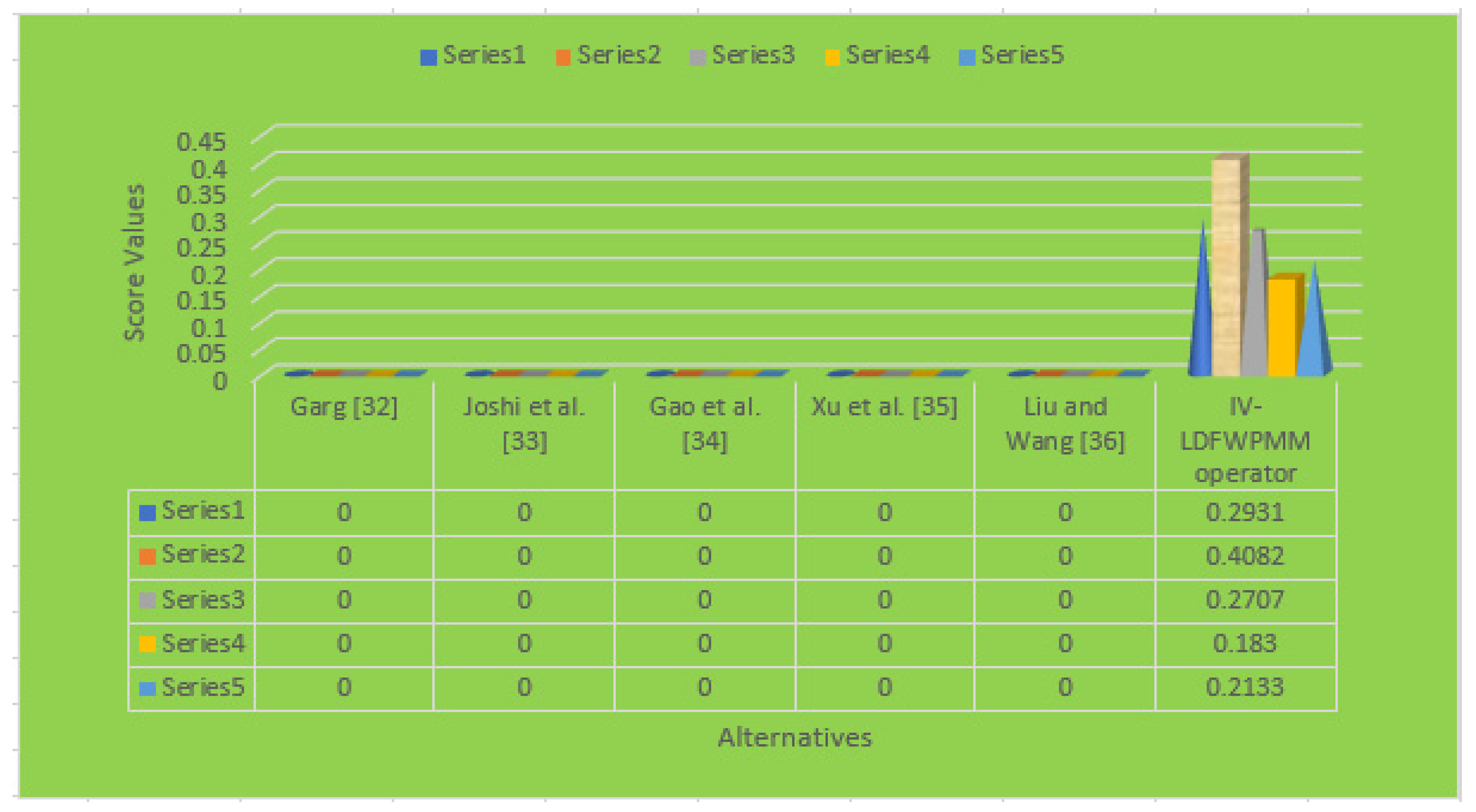
Garg [32]	Cannot be Formulated	Cannot be Formulated
Joshi et al. [33]	Cannot be Formulated	Cannot be Formulated
Gao et al. [34]	Cannot be Formulated	Cannot be Formulated
Xu et al. [35]	Cannot be Formulated	Cannot be Formulated
Liu and Wang [36]	Cannot be Formulated	Cannot be Formulated
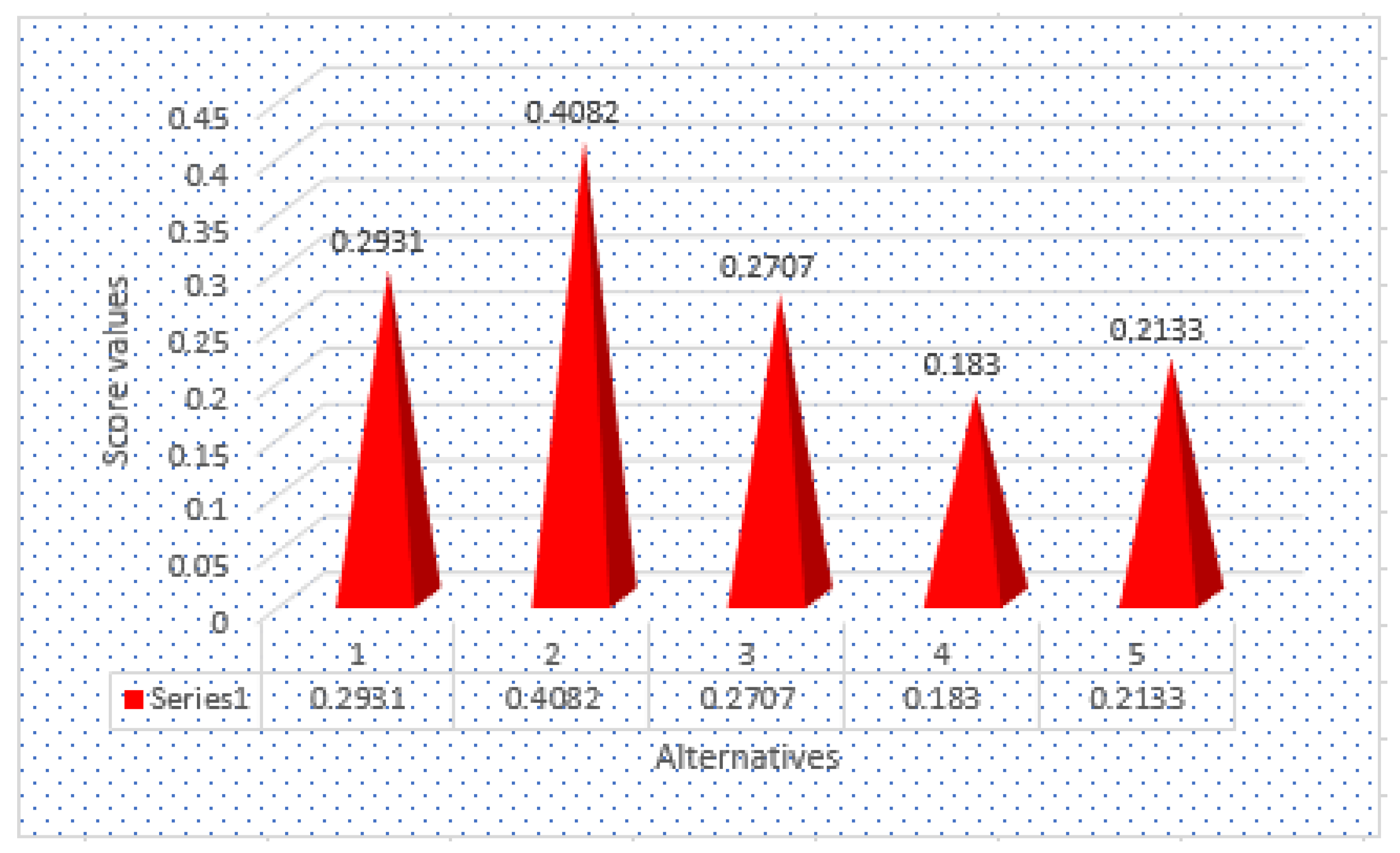
IV-LDFWPMM Operator	0.2931, 0.4082, 0.2707, 0.1830, 0.2133	AT− 2 > AT − 1 > AT − 3 > AT − 5 > AT − 4

gives a comparison with some existing operators [32,33,34,35,36], and the geometrical interpretation of the result is depicted in Figure 3.

Hence, it is obvious that the developments presented in the previous works [32,34,35] exhibit serous weaknesses due to their mathematically invented forms. Due to the demonstrated weaknesses of IV-IFSs, IV-PFSs, and IV-QROFSs, it is practically impossible to compare them with the tools proposed here.

6. Conclusions

Numerous authors dealt generally with the principles of fuzzy sets. The properties of IV-QROFSs and LDFS have also attracted a great deal of attention. Based on the presented work, the main achievements can be summarized as follows:

• The principle of IV-LDFS and its algebraic laws were introduced.
• The IV-LDFPMM and IV-LDFWPMM operators were introduced and their properties discussed to determine the strength and consistency of the operators.
• A MADM technique is presented in combination with the introduced operators, and the numerical examples demonstrated its advantages.
• Finally, a comparative analysis of the presented and other operators was discussed.

In the future, the presented work will be enriched by modifications of the principle of Pythagorean m-polar fuzzy sets [37,38], TOPSIS technique [39], T-spherical fuzzy sets [40], complex T-spherical fuzzy sets [41,42], complex neutrosophic sets [43,44], complex neutrosophic graph [45], complex neutrosophic lattice [46], non-cooperative behavior management [47,48], and decision-making procedures [49,50].

References

- Zadeh, L.A. Fuzzy sets. Infor. Control 1965, 8, 338–353. [Google Scholar] [CrossRef] [Green Version]
- Atanassov, K. Intuitionistic fuzzy sets. Fuzzy Sets Syst. 1986, 20, 87–96. [Google Scholar] [CrossRef]
- Bloch, I. Lattices of fuzzy sets and bipolar fuzzy sets, and mathematical morphology. Inf. Sci. 2011, 181, 2002–2015. [Google Scholar] [CrossRef]
- Muhammad, L.J.; Badi, I.; Haruna, A.A.; Mohammed, I.A. Selecting the Best Municipal Solid Waste Management Techniques in Nigeria Using Multi Criteria Decision Making Techniques. Rep. Mech. Eng. 2021, 2, 180–189. [Google Scholar] [CrossRef]
- Karamaşa, Ç.; Karabasevic, D.; Stanujkic, D.; Kookhdan, A.; Mishra, A.; Ertürk, M. An extended single-valued neutrosophic AHP and MULTIMOORA method to evaluate the optimal training aircraft for flight training organizations. Facta Univ. Ser. Mech. Eng. 2021, 19, 555–578. [Google Scholar] [CrossRef]
- Ramakrishnan, K.R.; Chakraborty, S. A cloud TOPSIS model for green supplier selection. Facta Univ. Ser. Mech. Eng. 2020, 18, 375–397. [Google Scholar] [CrossRef]
- Milosevic, T.; Pamucar, D.; Chatterjee, P. Model for selecting a route for the transport of hazardous materials using a fuzzy logic system. Mil. Tech. Cour. 2021, 69, 355–390. [Google Scholar]
- Milovanovic, V.R.; Aleksic, A.V.; Sokolovic, V.S.; Milenkov, M.A. Uncertainty modeling using intuitionistic fuzzy numbers. Mil. Tech. Cour. 2021, 69, 905–929. [Google Scholar]
- Yang, J.; Yao, Y. A three-way decision-based construction of shadowed sets from Atanassov intuitionistic fuzzy sets. Inf. Sci. 2021, 577, 1–21. [Google Scholar] [CrossRef]
- Jana, C.; Pal, M. Application of bipolar intuitionistic fuzzy soft sets in decision-making problem. Int. J. Fuzzy Syst. Appl. IJFSA 2018, 7, 32–55. [Google Scholar] [CrossRef]
- Yager, R.R. Pythagorean membership grades in multicriteria decision making. IEEE Trans. Fuzzy Syst. 2013, 22, 958–965. [Google Scholar] [CrossRef]
- Garg, H. A novel improved accuracy function for interval-valued Pythagorean fuzzy sets and their applications in the decision-making process. Int. J. Intell. Syst. 2017, 32, 1247–1260. [Google Scholar] [CrossRef]
- Peng, X.; Yang, Y. Fundamental properties of interval-valued Pythagorean fuzzy aggregation operators. Int. J. Intell. Syst. 2016, 31, 444–487. [Google Scholar] [CrossRef]
- Naeem, K.; Riaz, M.; Afzal, D. Pythagorean m-polar Fuzzy Sets and TOPSIS method for the Selection of Advertisement Mode. J. Intell. Fuzzy Syst. 2019, 37, 8441–8458. [Google Scholar] [CrossRef]
- Riaz, M.; Naeem, K.; Afzal, D. Pythagorean m-polar fuzzy soft sets with TOPSIS method for MCGDM. Punjab Univ. J. Math. 2020, 52, 21–46. [Google Scholar]
- Chen, T.Y. New Chebyshev distance measures for Pythagorean fuzzy sets with applications to multiple criteria decision analysis using an extended ELECTRE approach. Expert Syst. Appl. 2020, 147, 113164–113178. [Google Scholar] [CrossRef]
- Yager, R.R. Generalized orthopair fuzzy sets. IEEE Trans. Fuzzy Syst. 2016, 25, 1222–1230. [Google Scholar] [CrossRef]
- Garg, H. A new possibility degree measure for interval-valued q-rung orthopair fuzzy sets in decision-making. Int. J. Intell. Syst. 2021, 36, 526–557. [Google Scholar] [CrossRef]
- Liu, Z.; Wang, X.; Li, L.; Zhao, X.; Liu, P. Q-rung orthopair fuzzy multiple attribute group decision-making method based on normalized bidirectional projection model and generalized knowledge-based entropy measure. J. Ambient Intell. Humaniz. Comput. 2021, 12, 2715–2730. [Google Scholar] [CrossRef]
- Khan, M.J.; Kumam, P.; Shutaywi, M. Knowledge measure for the q-rung orthopair fuzzy sets. Int. J. Intell. Syst. 2021, 36, 628–655. [Google Scholar] [CrossRef]
- Papadakis, V.M.; Lioukas, S.; Chambers, D. Strategic decision-making processes: The role of management and context. Strateg. Manag. J. 1998, 19, 115–147. [Google Scholar] [CrossRef]
- Kushwaha, D.K.; Panchal, D.; Sachdeva, A. Risk analysis of cutting system under intuitionistic fuzzy environment. Rep. Mech. Eng. 2020, 1, 162–173. [Google Scholar] [CrossRef]
- Garg, H. CN-q-ROFS: Connection number-based q-rung orthopair fuzzy set and their application to the decision-making process. Int. J. Intell. Syst. 2021, 36, 3106–3143. [Google Scholar] [CrossRef]
- Sarkar, A.; Biswas, A. Dual hesitant q-rung orthopair fuzzy Dombi t-conorm and t-norm based Bonferroni mean operators for solving multicriteria group decision-making problems. Int. J. Intell. Syst. 2021, 36, 3293–3338. [Google Scholar] [CrossRef]
- Liu, D.; Huang, A. Consensus reaching process for fuzzy behavioral TOPSIS method with probabilistic linguistic q-rung orthopair fuzzy set based on correlation measure. Int. J. Intell. Syst. 2020, 35, 494–528. [Google Scholar] [CrossRef]
- Ali, M.I. Another view on q-rung orthopair fuzzy sets. Int. J. Intell. Syst. 2018, 33, 2139–2153. [Google Scholar] [CrossRef]
- Riaz, M.; Hashmi, M.R. Linear Diophantine fuzzy set and its applications towards multi-attribute decision-making problems. J. Intell. Fuzzy Syst. 2019, 37, 5417–5439. [Google Scholar] [CrossRef]
- Almagrabi, A.O.; Abdullah, S.; Shams, M.; Al-Otaibi, Y.D.; Ashraf, S. A new approach to q-linear Diophantine fuzzy emergency decision support system for COVID19. J. Ambient. Intell. Humaniz. Comput. 2021, 1–27. [Google Scholar] [CrossRef]
- Ayub, S.; Shabir, M.; Riaz, M.; Aslam, M.; Chinram, R. Linear Diophantine Fuzzy Relations and Their Algebraic Properties with Decision Making. Symmetry 2021, 13, 945. [Google Scholar] [CrossRef]
- Parimala, M.; Jafari, S.; Riaz, M.; Aslam, M. Applying the Dijkstra Algorithm to Solve a Linear Diophantine Fuzzy Environment. Symmetry 2021, 13, 1616. [Google Scholar] [CrossRef]
- Atanassov, K.T.; Gargov, G. Interval-valued intuitionistic fuzzy sets. Fuzzy Sets Syst. 1989, 31, 343–349. [Google Scholar] [CrossRef]
- Garg, H. A novel accuracy function under interval-valued Pythagorean fuzzy environment for solving multicriteria decision-making problems. J. Intell. Fuzzy Syst. 2016, 31, 529–540. [Google Scholar] [CrossRef]
- Joshi, B.P.; Singh, A.; Bhatt, P.K.; Vaisla, K.S. Interval-valued q-rung orthopair fuzzy sets and their properties. J. Intell. Fuzzy Syst. 2018, 35, 5225–5230. [Google Scholar] [CrossRef]
- Gao, H.; Ju, Y.; Zhang, W.; Ju, D. Multi-Attribute Decision-Making Method Based on Interval-Valued q-Rung Orthopair Fuzzy Archimedean Muirhead Mean Operators. IEEE Access 2019, 7, 74300–74315. [Google Scholar] [CrossRef]
- Xu, W.; Shang, X.; Wang, J.; Li, W. A novel approach to multi-attribute group decision-making based on interval-valued intuitionistic fuzzy power Muirhead mean. Symmetry 2019, 11, 441. [Google Scholar] [CrossRef] [Green Version]
- Liu, P.; Wang, P. Some improved linguistic intuitionistic fuzzy aggregation operators and their applications to multiple attribute decision making. Int. J. Inf. Technol. Decis. Mak. 2017, 16, 817–850. [Google Scholar] [CrossRef]
- Riaz, M.; Hashmi, M.R. Soft rough Pythagorean m-polar fuzzy sets and Pythagorean m-polar fuzzy soft rough sets with application to decision-making. Comput. Appl. Math. 2020, 39, 1–36. [Google Scholar] [CrossRef]
- Naeem, K.; Riaz, M.; Karaaslan, F. Some novel features of Pythagorean m-polar fuzzy sets with applications. Complex Intell. Syst. 2021, 7, 459–475. [Google Scholar] [CrossRef]
- Mahmoodzadeh, S.; Shahrabi, J.; Pariazar, M.; Zaeri, M.S. Project selection by using fuzzy AHP and TOPSIS technique. World Acad. Sci. Eng. Technol. 2007, 30, 333–338. [Google Scholar]
- Liu, P.; Zhu, B.; Wang, P. A multi-attribute decision-making approach based on spherical fuzzy sets for Yunnan Baiyao’s R&D project selection problem. Int. J. Fuzzy Syst. 2019, 21, 2168–2191. [Google Scholar]
- Karaaslan, F.; Dawood, M.A.D. Complex T-spherical fuzzy Dombi aggregation operators and their applications in multiple-criteria decision-making. Complex Intell. Syst. 2021, 7, 2711–2734. [Google Scholar] [CrossRef] [PubMed]
- Nasir, A.; Jan, N.; Yang, M.S.; Khan, S.U. Complex T-spherical fuzzy relations with their applications in economic relationships and international trades. IEEE Access 2021, 9, 66115–66131. [Google Scholar] [CrossRef]
- Ali, M.; Smarandache, F. Complex neutrosophic set. Neural Comput. Appl. 2017, 28, 1817–1834. [Google Scholar] [CrossRef] [Green Version]
- Dat, L.Q.; Thong, N.T.; Ali, M.; Smarandache, F.; Abdel-Basset, M.; Long, H.V. Linguistic approaches to interval complex neutrosophic sets in decision making. IEEE Access 2019, 7, 38902–38917. [Google Scholar] [CrossRef]
- Quek, S.G.; Broumi, S.; Selvachandran, G.; Bakali, A.; Talea, M.; Smarandache, F. Some results on the graph theory for complex neutrosophic sets. Symmetry 2018, 10, 190. [Google Scholar] [CrossRef] [Green Version]
- Singh, P.K. Complex neutrosophic concept lattice and its applications to air quality analysis. Chaos Solitons Fractals 2018, 109, 206–213. [Google Scholar] [CrossRef] [Green Version]
- Gao, Y.; Zhang, Z. Consensus reaching with non-cooperative behavior management for personalized individual semantics-based social network group decision making. J. Oper. Res. Soc. 2021, 1–18. [Google Scholar] [CrossRef]
- Zhang, Z.; Li, Z.; Gao, Y. Consensus reaching for group decision making with multi-granular unbalanced linguistic information: A bounded confidence and minimum adjustment-based approach. Inf. Fusion 2021, 74, 96–110. [Google Scholar] [CrossRef]
- Zhang, Z.; Guo, C.; Martínez, L. Managing multi granular linguistic distribution assessments in large-scale multiattribute group decision making. IEEE Trans. Syst. Man Cybern. Syst. 2016, 47, 3063–3076. [Google Scholar] [CrossRef] [Green Version]
- Zhang, Z.; Kou, X.; Yu, W.; Gao, Y. Consistency improvement for fuzzy preference relations with self-confidence: An application in two-sided matching decision making. J. Oper. Res. Soc. 2021, 72, 1914–1927. [Google Scholar] [CrossRef]