
Sources of Economic Growth in Zambia, 1970–2013: A Growth Accounting Approach


1
Department of Agricultural and Resource Economics, Colorado State University, Fort Collins, CO 80523, USA
2
Department of Agricultural Economics, Oklahoma State University, Stillwater, OK 74078, USA
3
Department of Agricultural Economics and Extension, The University of Zambia, Box 32379, Lusaka 10101, Zambia
*
Author to whom correspondence should be addressed.
Economies 2017, 5(2), 15; https://doi.org/10.3390/economies5020015
Submission received: 24 February 2017
/
Revised: 29 April 2017
/
Accepted: 4 May 2017
/
Published: 11 May 2017
Abstract
:Most empirical work on sources of economic growth for different countries lack country-specific empirical evidence to guide policy choices in individual developing countries and previous studies of factor productivity tend to focus on the entire economy or a single sector. This provides fewer insights about a country’s structural evolution. Unlike previous studies, our study builds on this by taking a more comprehensive approach in estimating Zambia’s sources of economic growth by sectors—agriculture, industry, and service—in a systematic manner that yields insights into the country’s sources of structural transformation. We use recently developed growth accounting tools to explicitly determine sources of economic growth at both national and sectoral levels in Zambia between 1970 and 2013. We use data from World Development Indicators and Zambia’s Central Statistical Office. Results indicate that, on average, total factor productivity (TFP) contributes about 5.7% to economic growth. Sectoral analysis shows that agriculture contributes the least to GDP and that, within each sector, factors that contribute to growth differ. Structural transformation has been slow and contributed to the observed inefficiency. We outline the implications of the observed growth and provide recommendations.
JEL Classification:
O40; O41; O551. Introduction
Economic growth, an important concept of development economics, is a crucial step in the development ladder and the achievement of a high and sustainable rate of economic growth remains a central theme for many world economies. Recent years have witnessed a growing debate on determinants of economic growth and income distribution across countries. Empirical studies have shown that economic growth rates differ among countries due to technology adoption (Romer 1986; Aghion and Howitt 1992), varying determinants of efficiency of savings and investment (World Bank 1990) and differing rates of accumulation of physical and human capital resources (Solow 1956; Mankiw et al. 1992). For least-developed countries (LDCs) in Sub-Saharan Africa (SSA), availability of natural resources, poor economic policies, access to the sea, tropical climate, volume of exports, a longer life expectancy and increased investment rates are some of the factors that drive economic growth (Sachs and Warner 1997; Upreti 2015).
Though the amount of empirical papers investigating the sources of economic growth for different countries has expanded significantly, country-specific empirical evidence to guide policy choices in individual developing countries remains arcane (Chirwa and Odhiambo 2016). Policy makers and political economists in LDCs strive to tackle the enigma of slow economic growth rates (or lack of it) recorded by their economies. For example, the empirical evidence of slow economic growth rate for African economies is generally sourced from cross-country regressions, which fail to take into account of individual country diversity of experiences (Altug et al. 2008; Anyanwu 2014; Chirwa and Odhiambo 2016). Such studies could be of vast importance at regional level, but not at individual country level. In addition, little empirical work has closely examined determinants of economic growth for most developing countries and Zambia is no exception. For example, we are aware only of Chirwa and Odhiambo (2016) that empirically determine Zambia’s macroeconomic determinants of economic growth. Their study does not reveal factor productivity of the Zambian economy or any of the broad economic sectors i.e. agriculture, industry and service. Determining factor productivity could be crucial to helping policy makers and government design evidence-based sectoral policy that requires data from both physical and social sciences.
Further, previous studies of factor productivity tend to focus on the entire economy or a single sector of the economy. As Herrendorf et al. (2013) and Johnston (1970) have pointed out, a fundamental feature of growth is a decline in the agriculture sector and labor share in total value-added, an increase in the service sector in value-added and labor, while industry’s share may rise or fall depending on a number of factors. Thus, this study aims to take a more comprehensive approach by estimating Zambia’s sources of economic growth by sectors—agriculture, industry, and service—in a systematic manner that yields insights into the country’s sources of structural transformation. Our integrated approach to measuring factor productivity provides insights into the sources of structural transformation not otherwise obtainable from just an economy-wide or a single sector approach. We do so by employing a sectoral analysis mainly separated into two time periods—before the structural adjustment programs (1970–1991) and post-reforms (1992–2013). This distinction allows us to capture underlying differences in sectoral contributions to economic growth, which is extremely important as pre- and post-reform periods have had important implications on Zambia’s economic growth (Ndulo and Mudenda 2010).
Zambia is a LDC located in SSA and agriculture is the mainstay of about 70% of the population (United Nations Development Programme 2015). Approximately the same fraction of people whose primary economic activity is agriculture live in the rural areas and about 77% of them are poor (Central Statistical Office 2016). Agriculture, further, contributes, on average, about 18% to GDP. For the industry sector, it has varied in magnitude since Zambia’s independence in 1964. Ndulo and Mudenda (2010) showed that industry sector contributed 6% to Gross Domestic Product (GDP) but its contribution rose significantly between 1964 and 1975. Its contribution to the share of exports is mainly concentrated in total non-traditional exports though it was quite volatile over the years (Ndulo and Mudenda 2010). The service sector is Zambia’s largest formal employment sector and its growth between 1965 and 2002 stood at 3% per annum and strong performance in the tourism, transport, and telecommunications sectors have contributed to the continued rise in the services sector (Central Statistical Office 2016).
Taken together, these facts briefly reflect the importance of the three sectors to Zambia’s economy. The achievement of the Zambian government’s goal of food security and efficiency in both industry and service sectors may have to rely on improved productivity in all three sectors. It follows that measurement and therefore a comparison of TFP in all the sectors is crucial for providing insightful answers to questions such as where has resource efficiency been concentrated among agriculture, industry, and the service-producing sectors? To the best of our knowledge, no empirical studies exist that provide TFP estimates in both industry and services sectors for Zambia, perhaps due in part to unavailability or considerable doubt of the how reliable existing data are. Some researchers have recently made considerable efforts to estimating productive efficiency in agriculture but none of them have explicitly incorporated estimates of agricultural TFP in Zambia. They have instead used partial measures such as technical efficiency in crop production in a selected region in Zambia (see: Chiona et al. 2014; Musaba and Bwacha 2014; Ng’ombe and Kalinda 2015; Abdulai and Abdulai 2015). Though these measures are useful for providing sub-sectoral perspectives, they do not provide a broad outlook of general productivity growth of the agricultural sector. Thus, the second objective of this study is to determine the sources of growth within each sector. Unlike some studies that consider only capital and labor, we include land in our analysis, which is a key resource for agriculture’s sectoral growth.
Our major contribution is the use of economic theory to guide estimation of sectoral resource stocks using secondary data sources, which in turn allows estimation of TFP. Unlike previous studies, this study mainly uses the recently developed growth accounting methods by Roe et al. (2014) to estimate total factor productivity underpinned by neoclassical growth theory. We use Roe et al. (2014)’s methodology because it facilitates the use of more easily available time series data than reliance on micro-level data that is seldom available across sectors of the economy.
In the following sections, we first present a brief background of the three sectors, the methodology and the data sources. We proceed to the results and discussion section and then the last section highlights the conclusions and policy implications.
2. Background
2.1. Agricultural Sector
Maize (Zea mays L.) dominates Zambia’s agriculture and its production dates back to the 16th Century, the period when Zambia’s main staple crops were sorghum (Sorghum bicolar L.) and millet (Eleusine coracana L.). Maize gradually replaced sorghum and millet as the country’s staple crops and by 1964, maize had already accounted for more than 60% of Zambia’s total planted area for major crops (Byerlee and Eicher 1997). Up to the early 1990s, the sector was still dominated by maize and lacked private sector participation in the areas of agricultural marketing, input supply and processing. In 1992, the Zambian government embraced agricultural sector policy reforms, as part of the general economic reforms that fell under pursuit of the structural adjustment programs. These were targeted at liberalizing the agricultural sector alongside promoting private sector participation in the agricultural supply chain (Ministry of Agriculture and Co-Operatives 2004). Since Zambia’s launch of the Comprehensive Africa Agricultural Development Program (CAADP) in 2006, the expectation has been that the agricultural sector would improve. CAADP is aimed at achieving and maintaining a higher path of agricultural-led economic growth in Africa and for Zambia; it is vital to supporting and strengthening implantation of national development plans such as the recent Sixth National Development Plan (SNDP) (Ministry of Agriculture 2017).
Zambia’s agriculture is dominated by smallholder farmers and is still underdeveloped (Chirwa and Odhiambo 2016). However, Zambia still has the potential to expand its agricultural production, owing to its massive resource endowment in arable land, labor and water resources. Bordered by eight countries and being a member of the Common Market for Eastern and Southern Africa (COMESA) and the Southern African Development Community (SADC) bolsters its market for agricultural produce. The country has access to the European Union agricultural markets through the Everything but Arms (EBA) initiative in addition to access to the U.S. market through the African Growth Opportunities Act (AGOA). By 2009, exports of agricultural products from Zambia to COMESA had reached a total of 125 million US$ and to the European Union a total of 147 million US$ (Ndulo and Mudenda 2010).
2.2. Industry Sector
After Zambia’s independence from Britain in 1964, the industry sector contributed about 6% to GDP and copper accounted for over 90% of foreign exchange. Between 1964 and 1975, the country experienced rapid economic growth relative to earlier periods and other countries in SSA. This growth rate was attributed to increased investments in industry sector whose proportion of total investment rose from about 7% in 1964 to about 12% in 1980 (Ndulo and Mudenda 2010). Between 1964 and 1991, the share of value added in the industry sector rose by 15% and manufactured goods also diversified.
Commonly manufactured commodities such as food and beverages reduced from 52% in 1970 to about 22% in 1980 while chemical products increased in the same period. However, manufactured commodities contributed about 0.7% to the total exports. These mainly comprised copper cable, menswear, sugar and molasses, cement, crushed stone and lime and explosives as of 1980 (Ndulo and Mudenda 2010). A summary of the contribution of output from the industry sector from 1992 to 2008 is presented in Table 1.
Following the structural adjustment programs in the 1990s, industry value added to GDP dropped from 15 to about 9.5% (Ndulo and Mudenda 2010). Inflation rose to 69% in the 1990s from about 11.6% in the 1980s. It averaged around 127% between 1990 and 1993. By 1995, inflation rate was about 25% and was maintained this way till 2000. The exchange rate rapidly depreciated and the real interest rates were negatively large (DiJohn 2010).
2.3. Services Sector
The Services sector captures the monetary value of such service as finance, communications, transport, distribution, health, education, tourism and foreign direct investment. We also consider trade services to encompass cross-border trade by both road and air transport. Between 1960 and 2002, about 90% of Zambia’s economic growth was attributed to service sector growth and since 2002, it has continued to contribute about 50% of GDP’s growth rate (Mattoo and Payton 2007).
The services sector’s growth rate was low before 2002 and Mattoo and Payton (2007) contend that government intervention and structural adjustment programs could be the causes. For example, the government had continued to regulate the telecommunications industry. The telecommunications sector had not been fully liberalized as the government continues to limit the number of players in the sector. In general, other changes in sub-sectors under the services sector have also contributed to changes in the services sector over the years. For example, the Consumer Unity and Trust Society (CUTS 2008) estimates that Zambia’s tourism sector’s contribution to GDP was about 2.4% from 2001 to 2006. The transport and communication sectors grew by 6.5% in 2004. CUTS (2008) attribute this growth rate to increased economic output and activities in sectors such as agriculture and mining, with value added arising from a relatively active tourism sector. Being such a large sector, it follows that determining its productivity is necessary to understanding its efficiency and contribution to overall economic growth.
3. Methodology
3.1. Alternative TFP Estimation Methods
Estimation of TFP dates back to studies by Solow (1957) and for more than a decade, a share of empirical studies on TFP has expanded significantly. These studies have estimated TFP using different methodologies. Available methods include indexing methods, non-parametric approaches such as the Malmquist-type index, data envelopment analysis (DEA) and the parametric stochastic frontier analysis (SFA). Many statistical agencies, such as the U.S. Bureau of Labor Statistics use the Growth Accounting Techniques based on Törnqvist indices to determine market sector multifactor productivity. Despite a variety of estimation methods, estimation of TFP has a common feature: it is founded on the theory of a production function, which is commonly specified as a real-valued function of capital (K), labor (L) and technology. Technology is typically assumed to be Hicks neutral, exogenous and homogenous across countries.
Studies by Hayami and Ruttan (1985) and Wen (1993) used index methods, while Coelli and Rao (2005) use a DEA framework—an approach that uses mathematical programming techniques to evaluate the relative performance of a set of peer entities called decision-making units (DMU) that convert (one or more) inputs into (one or more) outputs. While indexing methods might be simple to apply, Wang et al. (2009) note that their main difficulty is in determining the kind of index to use. The DEA framework is a powerful tool but has its shortcomings. For example, it is not based explicitly on an assumed statistical model and thus the properties of the efficiency estimates are ambiguous (Greene 2008). Greene (2008) noted that the estimators from DEA framework do not naturally produce standard errors for the coefficients which SFA is able to. SFA pioneered by Aigner et al. (1977) and Meeusen and van den Broeck (1977), has also extensively been used to determine productive efficiency.
Greene (2008) shows that SFA possesses an advantage over DEA framework in production efficiency studies because it possesses the ‘stochastic’ aspect that enables it to handle more appropriately measurement problems and other stochastic influences that would elsewhere show up as sources of inefficiency. Despite that strength, Wang et al. (2009), notes that SFA is not free from endogeneity of independent variables and there exists some difficulty of estimation by maximum likelihood estimation. Our study does not delve into constant quality price indices and dual approaches to growth accounting as used by many.
3.2. Neo-Classical Theory and TFP Estimation
Following Roe et al. (2014), the approach permits establishing whether a sector contributes its “fair share” to economic growth and also provides insights into the effects of intermediate factors of production on economic growth thereby identification of TFP from Solow residual.1 Let nominal economy GDP at equilibrium be defined as:
where the nominal values added in this two sector-two final good (for simplicity) economy are the price terms pj, j = 1,2; Yn is value added, Y1, Y2 are output values, K is physical capital, H is human capital, rk for K and w for H are factor rental prices equal to their marginal value products at equilibrium2. Human capital adjusted labor is Mincer specification and is H(t) = L(t)P(t)e0.1St, where L is working age population, P is labor market participation rate and St is years of schooling and 0.1 is the rate of return to schooling. A GDP function can therefore be defined for an economy producing any number of final goods and that the GDP function could help to distinguish the importance of imported intermediate factors of production, such as energy, chemicals and transportation services among others. Assuming an economy with both nominal and real GDP values and a two sector economy employing neoclassical technologies to produce two final goods, Y1 and Y2, using the services of capital K, labor H and ex, the labor service augmentation is as follows (Roe et al. 2014):
Economic theory postulates that holding p1 and p2 constant, say their values in period t*, real GDP can be interpreted, denominated in period t* constant prices as:
Letting be the equilibrium value of good j in a small and open Hecksher-Ohlin (H-O) economy, the GDP value obtained equals the value obtained by solving the following problem for each period t. For simplicity, dropping the (t) notation, we obtain the following:
A is constant and the function G(.) is homogenous of degree one in prices and AH and K. By envelope properties of G(.) (see Woodland 1982), and considering Equation (2) in real terms, the left-hand side of Equation (2) is an appropriate aggregator of individual sector technologies . In short, an aggregator of the sector production function with their production “competitive” market-determined levels of inputs K, AH yielding K, AH is Equation (2) which is the GDP function equivalent to an aggregate production function regardless of its functional form. Following Roe et al. (2014), allowing prices to vary, the nominal price effect on changes on Yn would be as follows:
where . The value of is determined from the firm’s optimization problem:
where
Therefore with , we have:
By additional simplification, we obtain Equation (3):
where Sj is the sector shares in GDP. The last term in Equation (3) is the Solow residual. In order to deal with the price terms, Equation (3) is expressed as follows:3
with these results, Roe et al. (2014) establish the proposition that growth accounting with a multi-sector GDP function as the underlying construct gives identical results as an aggregate production function albeit without an aggregation problem. Further analytical illustrations to derive sectoral TFPs are presented in the appendix.
4. Data
Data used in this study come from the World Bank’s World Development Indicators (WDI) and Central Statistical Office (CSO)4—the national statistics bureau in Zambia. WDI did not have data on employment by sector. This is the only variable we supplement with CSO data on employment by each sector for the years that CSO conducted the labor survey. However, because CSO did also not have the employment data for all the years, we had to reconstruct and estimate for the missing years. Another series that had to be reconstructed was the Gross Fixed Capital Formation (details of the reconstruction and estimation are in the next sub-section). The rest of the series were complete. Finally, for economy-wide and sectoral level factor shares, we use the Global Trade Analysis Project (GTAP) values for 2007. There were no other credible estimates we could find for Zambia except these provided by GTAP as shown in Table 2. In total, our data have 29 variables observed over a period of 44 years (from 1970 to 2013).
Data Issues
Gross Fixed Capital Formation (or investment): Gross Fixed Capital Formation data were available in constant and current local currency units (LCU) as well as in percentage of GDP. However, the LCU data were missing for the period 1994–2009 and 2011–2013, whereas the percentage data are available for the entire period. Besides, for the years when both LCU and percentage data are available, these two categories of data do not add up. For instance, the percentage data suggest 21.1% of GDP is used for investment in 2010, while the LCU data suggest the investment amounts to 25.9% of GDP (174 million LCU out of 97,216 million LCU). For consistency, the percentage data were chosen instead of the LCU data, since the former are available for the entire period. That is, the investment data were re-constructed using the data on GDP and the percentage of investment in GDP.
Employment Share by Sector: The data on sectoral employment share is available only for the four years of 1990, 1998, 2000, and 2005 from the central statistical office. However, the data for the year of 1990 does not sum up to unit. Hence, the agricultural labor share in 1990 is reconstructed as a residual of other sectors’ labor share. Labor employment share in agriculture is regressed on the rural population ratio for the available four years, with R-squared value being 0.542. In addition, the industrial labor share is regressed on the urban population ratio, with R-squared value being 0.968. The missing labor share data for agriculture and industrial sectors are then estimated using the regression equations for, respectively, the rural and urban population ratios, which are available for the entire period. Finally, the labor share of the service sector is estimated as the residual of other sectors’ labor shares. While this could be a shortcoming, we used the best available approach to estimate the labor shares by sector, which we believe underprops our study’s novelty.
5. Results and Discussion
5.1. Economy-Wide Analysis
Table 3 shows economy-wide growth accounting results for different periods between 1971 and 2013. We separate the analysis into 5 time periods to capture the trend at shorter intervals as a way of describing the economy. Growth accounting analysis at the economy-wide level was implemented in a theoretical framework with exogenous rate of capital depreciation (δ = 0.035) for the period 1971–2013. An exogenous rate of depreciation is chosen mainly because we assume, plausibly so, that capital depreciation is not related to growth. Secondly, we estimated the model with an endogenous rate of capital depreciation without success in getting plausible results. Over the period, the economy grew, on average, by 3.2% annually, of which productivity increase (TFP) accounted for only 5.7% (0.0018/0.0319). This implies that most of GDP growth for the same period is attributed to the increases in input use.
Increase in labor force accounts for nearly half (49.8%) of the growth of GDP. Capital accumulation also plays an important role as its contribution (44.5%) to growth is closely behind that of labor. The growth of labor, in turn, can come from such factors as an increase in population and more people joining the labor force. Agricultural land growth contributed the least to GDP growth in this period (1970–2013) at around 0.3%. This is probably because new marginal lands that are less fertile are being brought into production as opposed to changes in land quality.
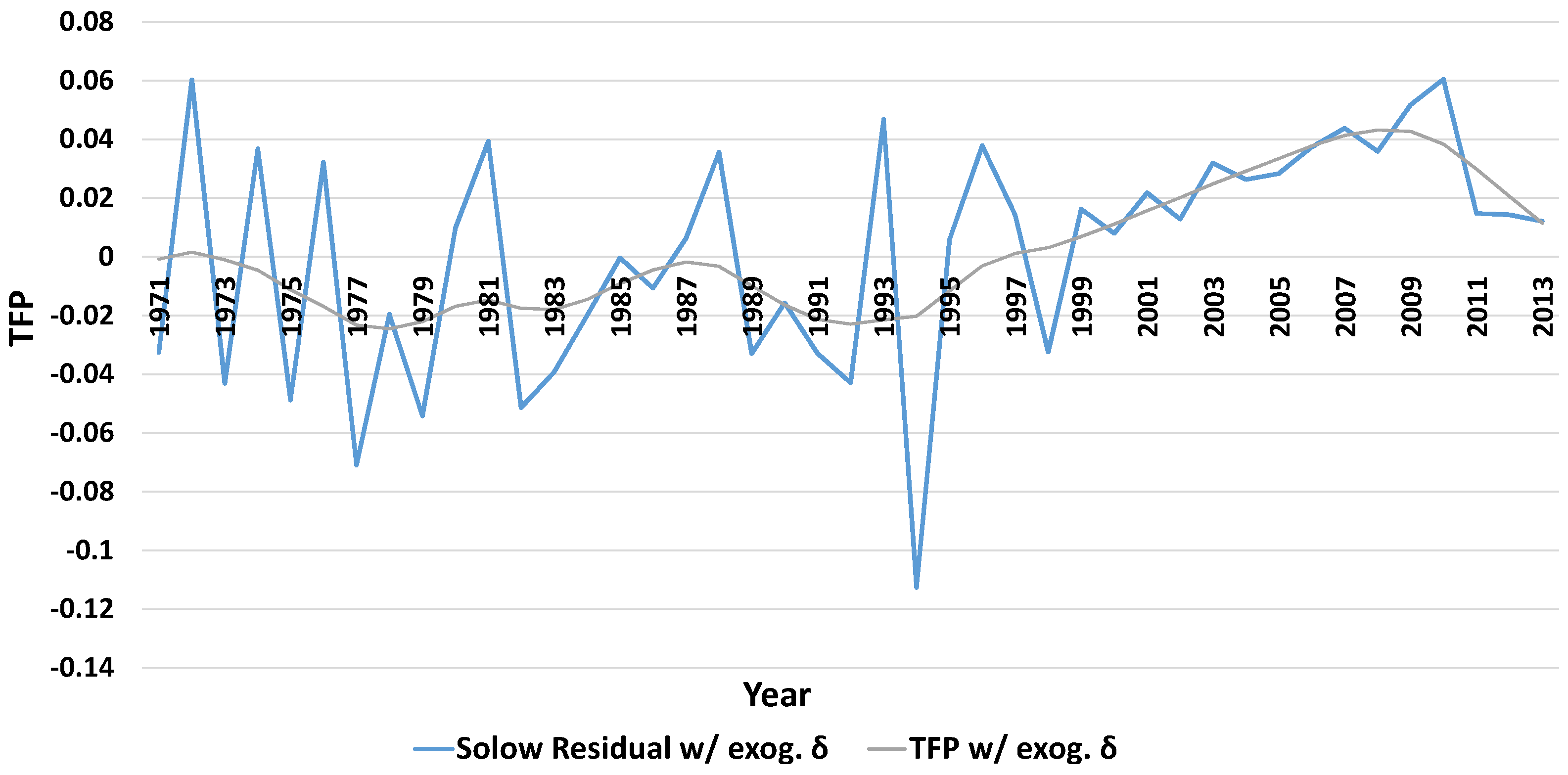
As indicated in Table 3, breaking the period into four intervals (1971–1980, 1981–1990, 1991–2000, and 2001–2013) shows the rising trend of productivity growth, captured by TFP. Between 1970 and 2000, TFP is negative indicating technological regress. This regress could have happened for several reasons among them government distortions in the market (Ndulo and Mudenda 2010), and the impact of HIV Aids in the 1990s (Haacker 2002). The mean TFP before 2000 is 0.001, implying that most of the growth is attributed to the increase in input use (mostly labor). However, productivity growth begins to accelerate from the year 2000. TFP growth amounts to 0.03 for the period 2001–2013. That is, 41% (GDP growth divided by Solow residual) of total GDP growth during the period is attributed to the improvement in resource productivity (TFP). This is also confirmed in Figure 1, which shows the trend of Solow residual and TFP over time. One reason for the low TFP before 2000 and high TFP after that could be increased education levels raising the workers’ skills (our labor variable does not have skills dimension, this is captured through TFP). This could the case for Zambia as the education sector was the focus of the first regime and the number of locally trained graduates increased sharply from independence in 1964 (Carmody 2004). During the same period (2001–2013), we see for the first-time capital stock growing tremendously and its contribution to growth surpassing that of labor. Some industries, perhaps, benefited from foreign direct investment and plausibly some of this capital that started flowing in came with state of the art technology to allow the country become more efficient—allowing for an increase in resource productivity.
Figure 2 illustrates the evolution of the economy in terms of capital deepening, defined as the capital to labor ratio with exogenous depreciation rate (δ). Before 2000, its trend was rather decreasing; implying economic growth (or lack thereof) during the same period was due to the growth of labor force and insufficient capital investment.
Capital deepening begins to accelerate, albeit slowly in the late 1990s and at a faster rate in the 2000s, increasing labor productivity and significantly improving growth performance during the period, as seen also in Table 3. During this same period (2000–2013), the economy in terms of GDP grew at 7.3% per annum, capital stock grew by 7.1% per annum and the labor force grew by 2.6% per annum. The capital contribution to GDP was highest in this same period at 2.7%, while labor growth rate and contribution to GDP declined slightly during the same period.
5.2. Sectoral Analysis
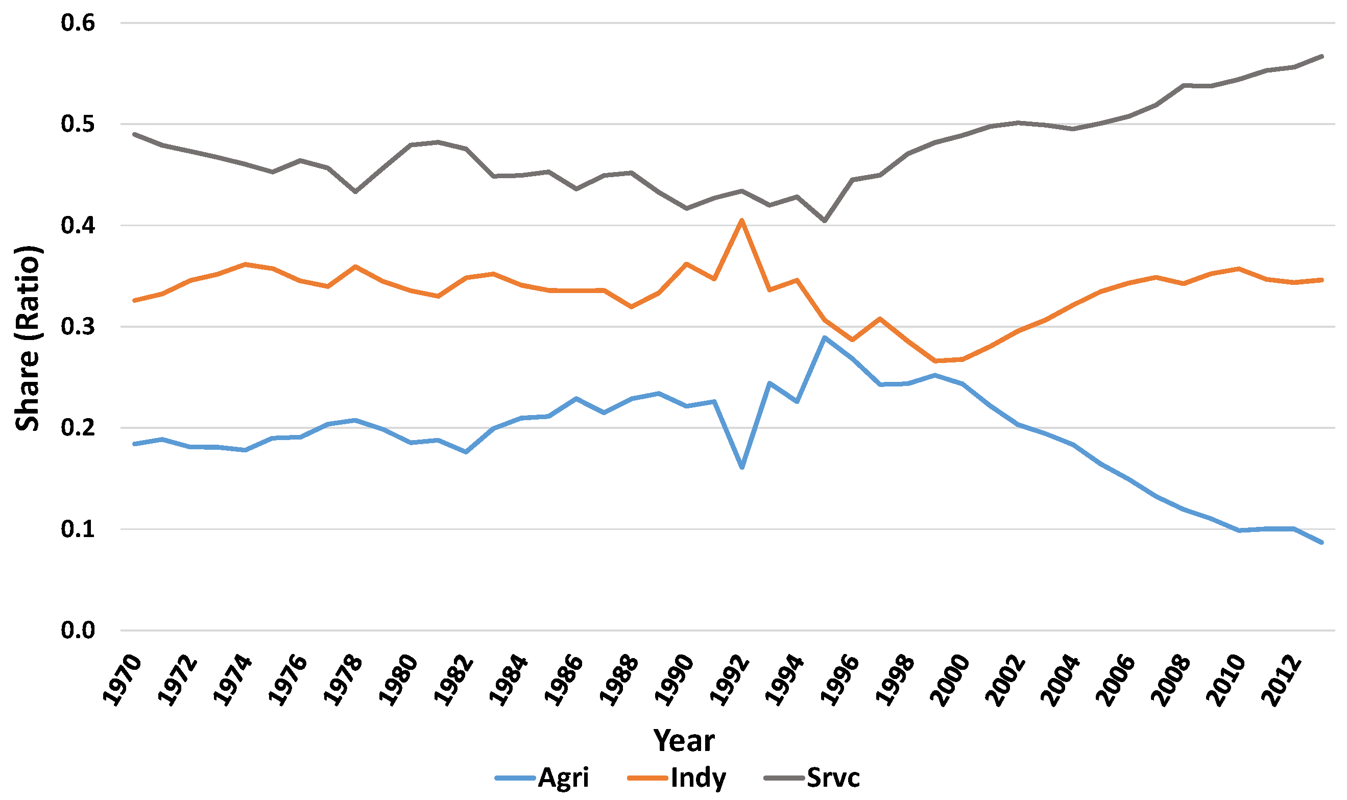
Next, we address whether the features of growth of the aggregate economy emanated from all sectors of the economy or they are specific to a particular sector. We disaggregate the data and analyze each sector’s contribution to GDP as well as the contribution to employment. Figure 3 shows the trend of GDP share by each sector for the period 1970–2013. Note that the typical structural transformation experienced by developing countries is observed only after 1995. Since 1995, agriculture’s of GDP shrunk, while the shares of other sectors are on the rise. Before 1995, however, little trend is observed in sector GDP shares.
Agriculture’s share of GDP also shrunk immediately after the 1990 attempted structural adjustment reforms, while industry’s share to GDP rose. However, this trend is reversed when the government changed most of its liberalization policies before starting them again in 1994. Most economies take a development path where industry and services sectors are expected to contribute more while agriculture declines as the country moves to a more technologically advanced level (Byerlee et al. 2009; Cervantes-Godoy and Brooks 2008; Herrendorf et al. 2013). Zambia seems to be on course in this line with both services and industry sectoral share contribution rising since 1999 while that of agriculture is falling. However, other authors argue that even industry begins to decline as the economy moves “traditional industry-intensive ‘Machine Age’ economy to a more services-intensive ‘Information Age’” (Rodrik 2015).
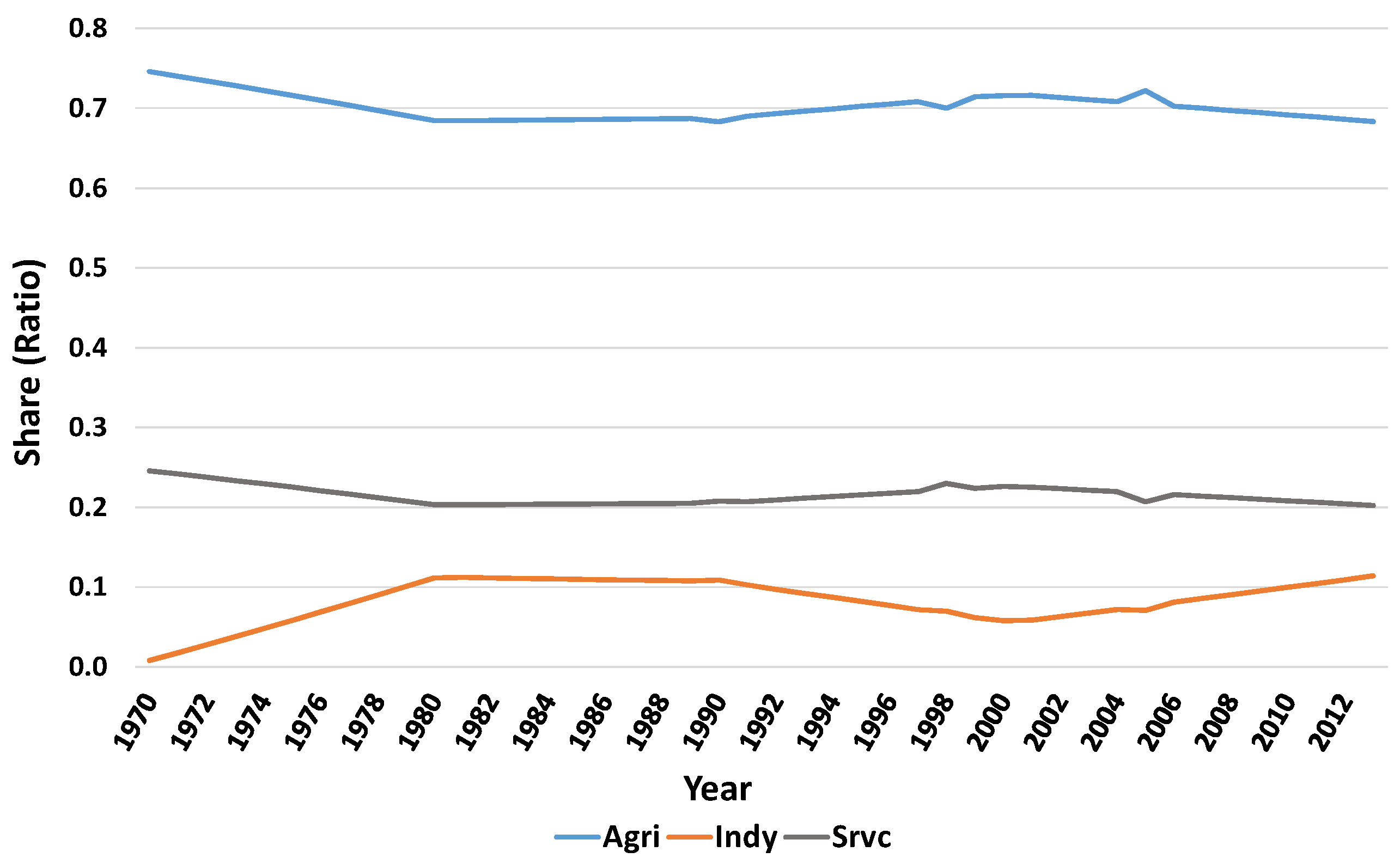
Figure 4 illustrates the trends of employment shares by each sector, which we find to be quite stable over time. It is noted, however, that the labor shares in agriculture and services have been gradually declining, while the labor share of the industrial sector has been increasing—these trends are non-monotonic. Particularly noteworthy is the extremely low productivity of agricultural labor. The agriculture sector accounts nearly for 70% of the labor force, but only produces 10% to 30% of value added. This is probably because more than 46% of the people engaged in agriculture have other sources of income or jobs that mainly include owning a business, non-agricultural wage and supplying labor to other farms (Bigsten and Tengstam 2008). This suggests that agriculture is a repository to which labor goes when it cannot find income elsewhere. In Table 4, we use the knowledge that a sector’s contribution, in percentage to growth in GDP should equal its share in GDP—“fair” share—if the economy is in long-run equilibrium. The “fair share” contribution is calculated as that sector’s mean contribution to GDP expressed as a proportion of the sum of the sectors’ contribution from 1971 to 2013.
Over the same period (1971–2013), GDP grew by 3.2% while agriculture, industry, and services grew by 2.1%, 3.4% and 3.7% respectively. The service sector grew the most, followed by industry and lastly agriculture with a difference of almost 10 percentage points between each of the two sectors (services and industry) and agriculture. Annual sector shares are 19.3% for agriculture, 33.3% for industry and 47.4% for services. Industry’s slow growth in the 1970s and 1980s was as result of the underdeveloped industrial base (Ndulo and Mudenda 2010). Mean contribution to GDP growth is 1.89% for services, 1.16% for industry and 0.6% for agriculture in declining order. The figures in parentheses are ‘fair share’ contribution. In theory, we expect that if the economy is in long-run equilibrium (steady state), labor and capital should grow at the same rate, since the capital per worker is constant (Abel et al. 2008).
Agriculture is contributing less than its fair share since its contribution of 16.4% is less than its share of 19.3% in economy GDP. The same applies for industry, while service is contributing more than its fair share with a contribution of 51.8% compared to its share of 47.4%. Agriculture lags by about 3% (19.3 − 16.4 = 2.9) while industry lags by 1.5% (33.3 − 31.8 = 1.5) in terms of contributing its fair share. Fair share is what we would expect in long-run equilibrium. We might call a sector contributing less than its share as a laggard sector. From this, we clearly see that agriculture is a laggard sector
5.3. Sectoral TFP Analysis
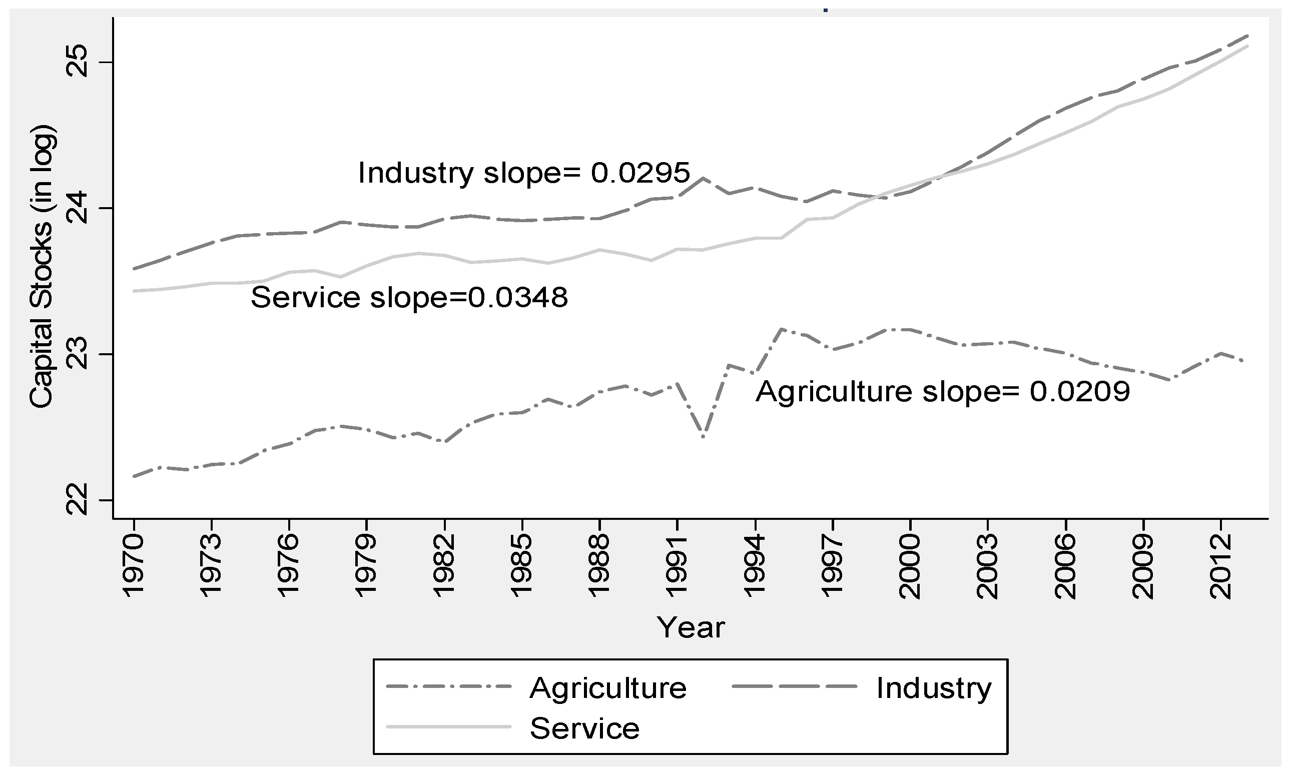
In Figure 5, sectoral capital stocks are plotted against time. The y-axis is capital stocks in natural logarithm and the slopes of the fit lines represent the annual compound rate of growth in the capital stock. As indicated by the slopes, all three sectors have different capital growth rates. From about 1998 the growth rates in service and industry sectors have almost been similar but agriculture capital stock has declined. Compound rate of growth (average slope) in the service sector is about 3.5% while for the industry sector, it is about 3%. Compound rate of growth in agriculture sector has been the slowest at about 2.1%. The fall in agriculture capital stocks coincided with government’s involvement in the output market through the Food Reserve Agency (FRA), which started buying maize in 1997, and the input subsidy program (Farmer Input Support Program) which started in 2002.
Studies by Mason and Myers (2013), and Mulungu and Chilundika (2016) have shown that this kind of government involvement crowded out the private sector and reduced investments in both the input and output markets. Sometimes economic growth may not be observed directly from labor and capital changes and two measures, capital deepening (capital stock per worker) and TFP capture such growth. In Table 5, we present capital deepening results for each sector. Capital deepening for agriculture is positive from 1971 to 1991, the period when Zambia had its first Republican President. From 1992 to 2013, capital deepening was declining. This could, among other factors, be due to an increase in the number of people employed in agriculture as confirmed by Figure 4 while the capital stock per agricultural worker has been decreasing from 1995 (Figure 5).
Capital deepening in industry decreased at 16% per annum during the period 1971 to 1991 and increased at about 2% per annum during the period 1992 to 2013. The low capital deepening in the first period could be a result of an economy that depended heavily on labor with outdated capital stock. Low savings and poor mechanisms of transferring the savings to investors is another plausible explanation. In that period, skilled labor, which is more efficient was scarce as higher education was still limited to only a few citizens. For example, at independence, Zambia only had 100 African educated graduates. Zambia, therefore, faced a critical shortage of skilled manpower in the years following independence.
This shortage was noticed by the first Republican president who we quote: “Expanding our Secondary School Education and paying greater attention to the requirements of university education, in order to produce qualified personnel… and help establish sound administrative cadres for upper and middle grades in government, commerce and industry, agriculture extension schemes and public works, for which good education is a must–has no substitute.”6
A close inspection of the data shows that this happened in the year 1972 when labor force grew by about 124% from the year 19707. Overall, we find capital deepening in industry during the period 1971–2013 to be declining at 6.8%. Service sector overall witnessed a rise in capital deepening of approximately 2% per annum over the same period (1971–2013). However, when separated into two time periods, capital deepening before 1991 is declining and increasing from 1992 to 2013. The number of people employed by the service sector rose steadily while capital stocks rose faster, at a rate almost equal to the rate in the industry sector.
Overall, growth rates in the labor force have not been so different between agriculture and service sectors (2.5% compared to 2.2%) while labor growth rate in the industry sector has been high at around 11% per annum. This increase in labor observed in the industry sector could possibly be arising from the increased production in the mining industry and the opening of new industries processing food items (Ndulo and Mudenda 2010; Carmody 2009). Industry and service sectoral capital stocks have been growing almost at the same rate of about 4%.
Table 6 shows results from the sectoral growth accounting. For each sector, we show the contribution of capital, labor, and TFP to the growth of the sector. For agriculture, we include the contribution of land. We divide time into three periods: (i) the pre-reform period of 1971–1991; (ii) the post-reform period from 1992 to 2013; and (iii) the overall (1970–2013). We do this so as to observe differences in the sectoral TFPs between the two periods. The first column in each period reports the point contribution to a sector’s growth and the second column reports the share of the factor’s contribution to the sector growth.
From the GTAP factor shares in Table 2, industry is the most capital-intensive sector followed by service sector while service is the most labor-intensive sector followed by agriculture. If a sector uses more capital, then capital should contribute more than labor combined with labor augmenting technological change in long-run equilibrium (Roe et al. 2014; Abel et al. 2008). In transition, however, this simply means capital should grow faster than Harrod plus labor force.
For instance, labor should account for the highest share of the growth in the services sector as should capital in the industry sector, assuming a long-run equilibrium. A close look at each sector’s growth rate in the first period shows that agriculture had the highest growth rate at approximately 2.4% per annum, compared to about 1.6% for the industry sector. The services sector has had the slowest growth in terms of value added, at about 0.7% per annum. In the post-reform era, following market liberalization, the private sector was allowed to stimulate economic gains and agriculture value added slowed down (to about 2% per annum) while the service sector made the highest gains (at 6.5% growth per annum). The industry sector was then growing at about 5.2% per annum.
Overall, we find that the service sector had grown more from 1971 to 2013, at about 3.7% per annum, than the industry sector, at 3.4% per annum, while agriculture has lagged behind on an average of 2.1% per annum. For agriculture, instead of only the two traditional inputs of labor and capital, there was growth in agricultural land contribution, which is minimal at 3.5%. Capital did not follow the pattern. Its contribution to sectoral growth matches the order of intensity of use across the sectors. Capital accounted for 65% of the growth in industry overall, followed by service where it accounted for about 37% while accounting for only a paltry (paltry because the cost of capital goods in this sector was still high) 30% in the agriculture sector.
When disaggregated into two time periods, we see that in the first-period industry’s growth is still mainly accounted for by capital but followed by service and not agriculture. In the second period, the pattern is the same. As for the overall period, capital contributes about 59% of the growth witnessed in the industry sector and about 44% and 33% of the growth in agriculture and service sectors, respectively.
Labor does not follow the theorized long-run pattern of intensity of use and contribution to growth equally. While the service sector is most labor-intensive, followed by agriculture, the contribution of labor to service sector growth is only 41% compared to about 132% contribution to the industry sector and lastly about 67% to agriculture. In the first period, labor contributes more to services but still less than the contribution to industry, which is at a staggering close to 500%8. This pattern changes from 1992 to 2013 as labor contributes more to agriculture followed by industry and then the service sector.
A closer look at the respective sectoral TFPs shows that only service sector has had a positive TFP with industry and agriculture having below zero TFPs. Industry has the lowest TFP at −0.033, followed by agriculture at −0.004 while service sector has the highest at 0.008. These TFPs account for −97%, 18% and 22.5% for industry, agriculture, and service sectors growth, respectively. Low TFPs for agriculture in developing countries are common in the literature (see, for example, Ogundari (2014), or El-Hadj (2013) for multi-country study). As can be seen from Figure 4, industry’s labor share in total employment has increased while those of agriculture and services have marginally declined during the period under review. Focusing on industry, we see that labor contributes more to industry growth than capital.
One plausible explanation for this low TFP in industry has to do with inefficiency in the sector. As shown from literature (for example El-Hadj 2013), openness in the economy leads to efficiency in the industry sector as non-efficient firms are pushed out of the production and the remaining ones are more efficient. However, with the protectionist policies of the 1970s–1990s, most firms that were government owned were inefficient and it is only after the liberalization and privatization of state-run parastatal institutions that the efficiency in the sector began to improve. This is matched by a positive TFP for industry in the second period (post-reform), in which it accounted for about 14% of the growth in the sector.
The second period (1992–2014) is also the time when the world experienced a commodity boom and rise in exports of minerals, which could explain the increase in productivity. Lack of openness also meant that the level of competition the firms were exposed to was low. The McKinsey Global Institute through its study of different countries finds a link between the level of competition that firms are exposed to and the productivity of the sector as measured by TFP (Manyika et al. 2010).
Service outperforming other sectors in the economy is not equally new. For example, Mukherjee (2013) finds that the service sector has had the highest TFP in India. The service sector—especially the telecommunications and transport sub-sectors—have continued to perform well, benefiting heavily from foreign direct investment.
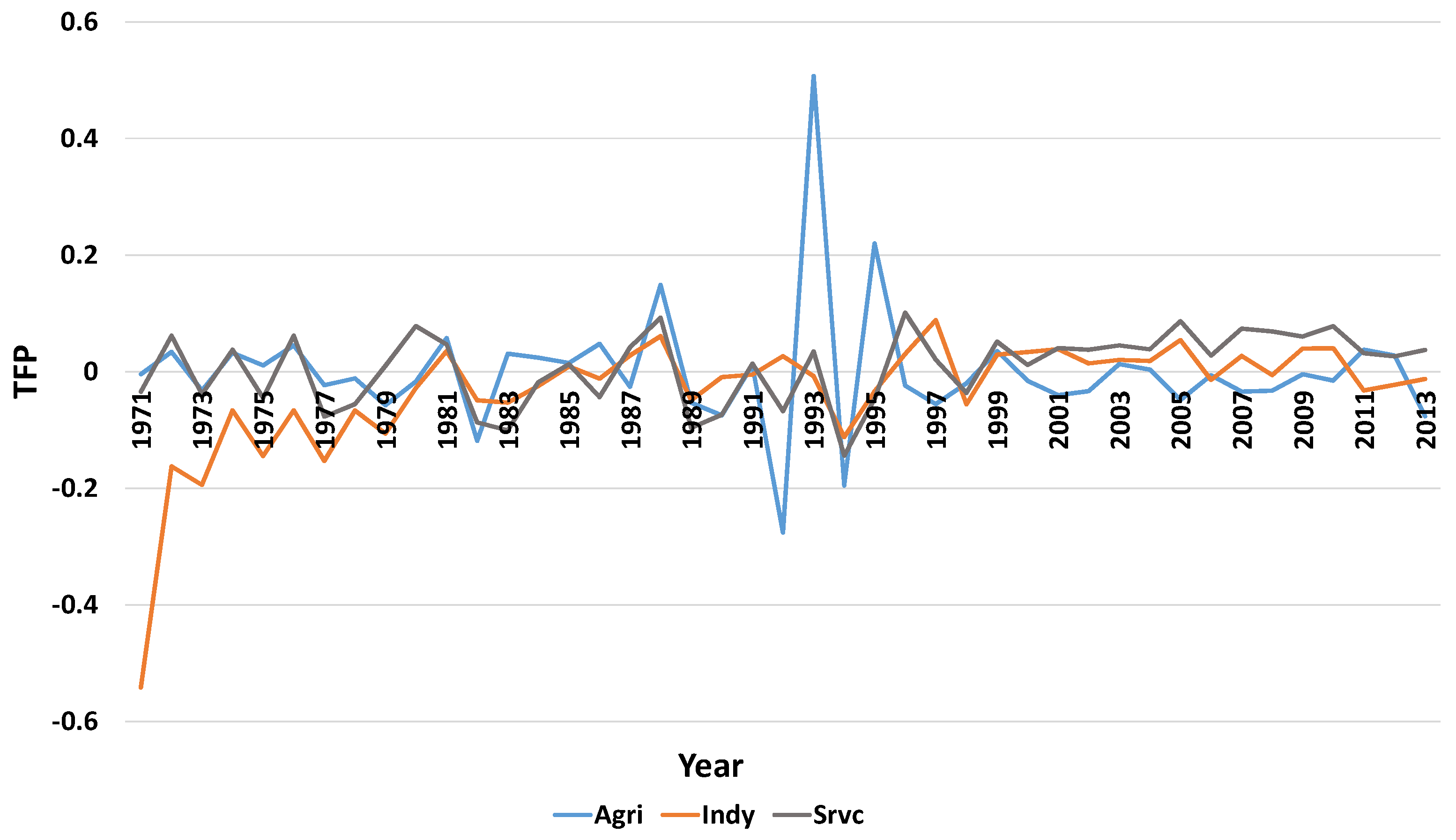
From Figure 6, we see that agricultural TFP has been the most volatile, especially around the early 1990s, at the inception of the structural adjustment programs and other reforms. Service TFP has been the most stable over time while industry TFP is extremely low in the 1970s and only improving around 1996 and stabilizing in the positive region from then on. According to Roe et al. (2014), it is expected of agriculture to have quite a volatile TFP given that it is dependent on weather. A case in point for Zambia is 1992 when it is lowest in the whole series. This is the year in which Zambia experienced the worst drought ever recorded to date.
Agriculture is generally considered a low labor productivity sector in developing countries and is used to measure the pace of development by focusing on the share of labor employed by the sector. In developed countries, the share of labor in agriculture is small while in developing countries almost everyone is employed in agriculture. Multiple reasons, which are also plausible in the case of Zambia, have been advanced for this low TFP (see, for example, Isaksson 2007; Aguiar et al. 2016). These include investment-dependent growth, differences in productivity arising from differences in economy-wide productivity, barriers to the use of modern intermediate inputs in agriculture, and policies that impact negatively on agriculture. These barriers reduce the incentives for farmers in poor countries to use modern inputs that are crucial for improving agricultural productivity. There is need for a more nuanced analysis to understand why TFP in agriculture has remained this low by probably understanding the underlying factors in the years it was high. The agricultural TFP has virtually remained stable around zero for much of the time except when it was very volatile. This low TFP includes recent years when Zambia has experienced increased agricultural production because of good weather.
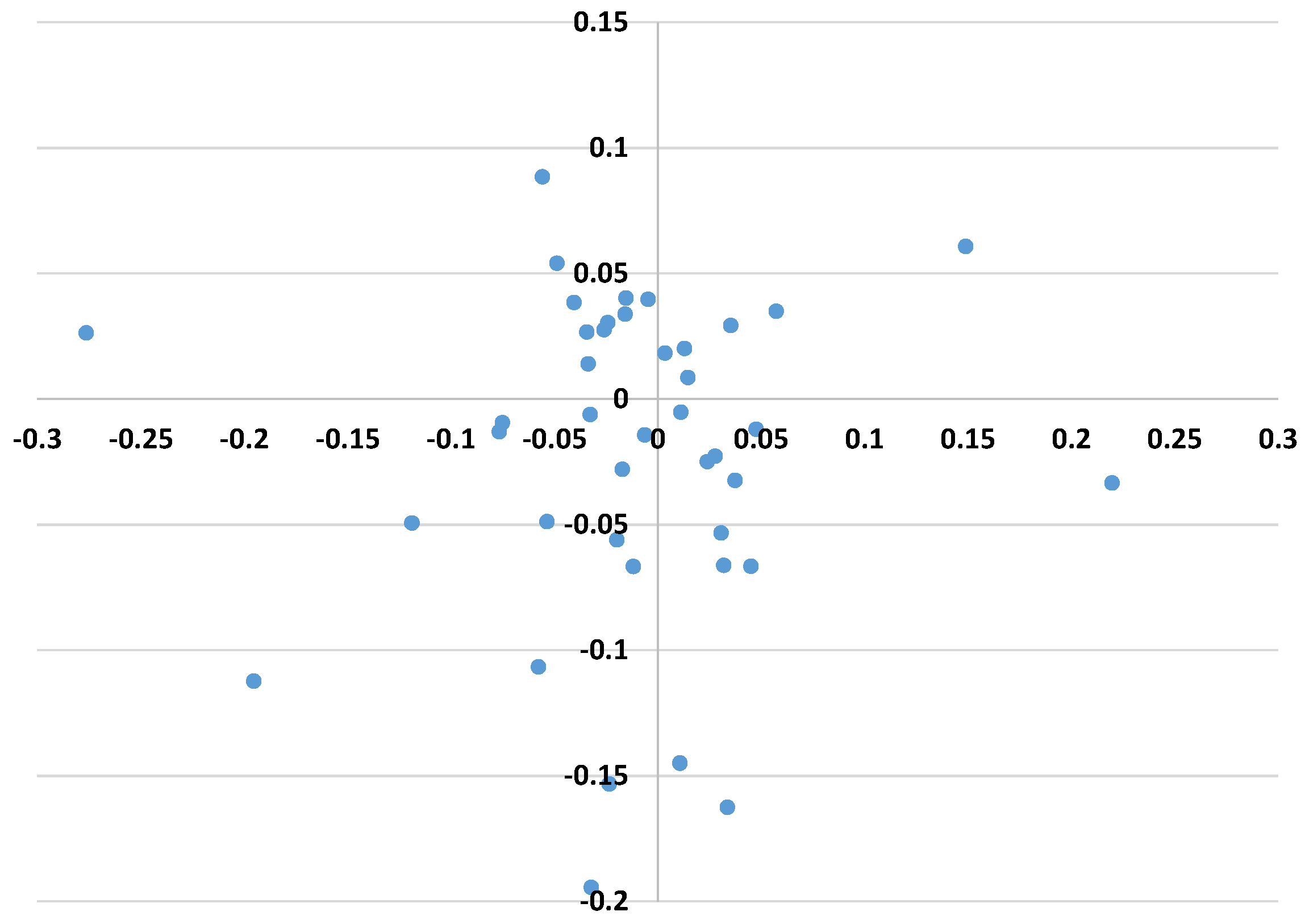
Figure 7 shows the scatter plots for agriculture TFP against industry while Figure 8 shows scatter plots for agriculture and service TFPs. From the graphs, observations appearing in the first and third quadrant suggest that TFP in one sector may spillover to TFP in the other sector. This means that there could be positive spillover effects from service to agriculture—for example a technological change in services spills over to TFP in agriculture, through, for example, lower cost transport services, more efficient marketing facilities and so on that could have improved under services. The positive relationship between agriculture and industrial sectors could come from the fact that as the industrial sector develops, it demands from the agriculture sector inputs and raw materials that go into manufacturing. Koo and Lou (1997) find that industry growth contributes to growth in the agriculture sector even though they model a two-sector economy. Even though this analysis on spillover is not conclusive, we feel it is a logical question to pose. As structural transformation continues and more labor is moved from agriculture to industry and services, there will be positive benefits for agriculture through the spillover effects.
6. Conclusions
This study uses the recently developed growth accounting tools by Roe et al. (2014) to determine the sources of growth in Zambia’s agriculture, industry and service sectors during the period 1970 and 2013. We use data from World Development Indicators and Zambia’s Central Statistical Office. Our results suggest that overall, capital and labor growth have been the main drivers of growth. TFP over the period 1970–2013 accounts for only 5.7% of the growth compared to labor growth, which accounts for around 50% of the growth. Agriculture employs more people than the two sectors with about 70% of the labor force employed in agriculture. This huge number also means that with low capital investments in the sector, capital deepening has been the lowest among the three sectors. Even though capital stocks have been rising, the rise cannot be compared to that observed in industry and services sectors.
Our results from sectoral analysis covering the pre-reform and the post-reform time periods tell two different stories. First, the pre-reform era was characterized by below zero TFP. Service TFP was below zero. Industry TFP was below zero as well. Second, the post-reform era saw services TFP increase significantly contributing about 22.5% to the growth of the sector probably because labor productivity increased in this sector. Industry TFP changed from negative in the pre-reform period to being positive in the post-reform period. Though industry was immediately hit hard after the reforms in the 1990s, there was a considerable gain in the 2000s that offsets this negative effect (Resnick and Thurlow 2014). Agriculture TFP stayed almost the same in both time-periods at around zero in the pre-reform years and just above zero after the reforms. Capital deepening in the sectors also differed across the two periods. Agriculture capital deepening was very low in both periods. Industry and services had negative capital deepening in pre-reform but had positive capital deepening in the post-reform era.
Overall, we find agriculture TFP as the most volatile especially around the early 1990s when there was a change of government and the new government began implementing structural adjustment programs. The volatility is also attributed to weather as more than 90% of the agricultural production in Zambia is rain-fed (Ministry of Agriculture and Co-Operatives 2004). In terms of analysis of contribution to growth and share of GDP, we find that agriculture contributes less than its fair-share to growth while service contributes more than its fair share despite the positive correlation with services and industry sectors. This low contribution to GDP combined with a low capital deepening (lower than services but higher than industry) suggests that there are factors that could be slowing down structural transformation. One factor that could be slowing down structural transformation is the land rights and tenure system in rural Zambia where 93% of the land is customary land without a title for the smallholder farmers who use it (Adams 2003). This tends to affect the reallocation of labor from agriculture to other sectors (De Janvry et al. 2015). Service seems to be the only sector performing well on contribution and productivity measures.
From our results, we suggest the following. Growth in agricultural sector could be attributed to mainly labor growth. There is need to attract capital in agriculture. Deliberate efforts must be made to allow farmers adopt new technologies and encourage the use of machinery. Even though there is zero tax on agricultural equipment, credit constraints have left most farmers unable to take advantage of this measure. Despite employing about 70% of the labor, agriculture contributes less to the economy and does not meet its fair share contribution. Labor productivity in a sector filled mainly with smallholder farmers is low. Policies to educate the population and reduce illiteracy levels, and encourage labor reallocation to more efficient sectors like services would help improve resource use in the economy overall. Resnick and Thurlow (2014) show that during the post-reform period, labor moved into agriculture which has low value-added per worker and this reduced the value added in the whole economy. Further, we suggest institutional and economic reforms as potential sources of sectoral productivity growth and that more research and development should be encouraged for perhaps a more detailed understanding of the factors affecting the growth of these sectors and determining the factors influencing the productivity at sector and national levels.
For efficient structural transformation, reforming land rights for farmers to allow them title deeds for security of ownership even without their presence is important. De Janvry et al. (2015) show that the key constraint imposed by insecure property rights is the requirement of continued presence and cultivation even when one is not productive. These secure lands would increase the efficiency of labor allocation by allowing and inducing less productive farmers to migrate into other sectors of the economy leaving more productive farmers to cultivate more land. The smallholder farmers who migrate would also receive benefits in the sectors that they migrate to (Adamopoulos and Restuccia 2014; De Janvry et al. 2015). When less productive smallholder farmers leave for other sectors, this would allow agricultural TFP to rise faster than in non-agriculture, so productivity will tend to rise and converge (Ranis and Fei 1961).
Acknowledgments
The authors would like to thank Forum for Agricultural Research in Africa (FARA) for financial support and University of Minnesota for technical support. We also thank Terry Roe for taking time to review an earlier draft of this paper. The authors also sincerely appreciate the comments of the editor, Ralf Fendel, and three anonymous reviewers.
Author Contributions
The paper is a joint contribution of the two authors.
Conflicts of Interest
The authors declare no conflict of interest.
Appendix A. Sectoral Output Contributions to GDP and TFPs adapted from Roe et al. (2014)
A.2. Estimation of Sectoral TFP
Following Roe et al. (2014), we first focus on theory used to guide our estimation of sectoral capital stocks. We then draw upon similar economic conditions underlying our growth accounting assumptions utilizing a sectoral version of the GDP function. To determine each sector’s TFP in a three-sector economy, we add to the H-O model another final good sector that employs labor capital and for a general case where a given factor, land denoted Z is fixed. The capital market clearing equation is:
As observed in Equation (A2), the term is the derivative of the indirect sector level profit function with respect to where:
where pa is agriculture’s output price and is assumed exogenous and like other prices, normalized to unity, while . Following Roe et al. (2014) and assuming neoclassical Cobb-Douglas production technologies, the capital market clearing equation becomes:
The rental share of land in total sector revenue is while agricultural sector’s supply function is . By substituting into the capital market clearing equation, we obtain the following
whose equivalence is
for the case where land, Z is constant. For our case where Z is variable, we the agricultural sector’s cost function
which results in the capital market clearing equation shown below9
Equation (A5) is identical to Equations (A3) and (A4). The equivalence is shown in Equation (A6)
where sectoral is calculated as follows
Consequently
Once the LHS terms of Equation (A5) are known, implicit rate of return on capital can be computed. Roe et al. (2014) observe that we require no knowledge of the fixed factor other than its shadow or rental value used in the calculation of or utilize the value reported in the Global Trade Analysis Project (GTAP) data set. Therefore, the Solow’s residual for the sector employing the fixed factor H with technology is
If data on land, Z(t) are unavailable, the effects of would be embodied in our estimate of Solow’s residual.
References
- Abdulai, Abdul Nafeo, and Awudu Abdulai. 2015. Allocative and scale efficiency among maize farmers in Zambia: A zero efficiency stochastic frontier approach. Applied Economics 48: 5364–78. [Google Scholar] [CrossRef]
- Abel, Andrew B., Ben S. Bernanke, and Dean Croushore. 2008. Macroeconomics, 6th ed. New York: Addison Wesley Longman. [Google Scholar]
- Adamopoulos, T., and D. Restuccia. 2014. The size distribution of farms and international productivity differences. The American Economic Review 104: 1667–97. [Google Scholar] [CrossRef]
- Adams, Martin. 2003. Land Tenure Policy and Practice in Zambia: Issues Relating to the Development of the Agricultural Sector. Draft Document for DFID. Lusaka: DFID. [Google Scholar]
- Aghion, Philippe, and Peter Howitt. 1992. A Model of Growth through Creative Destruction. Econometrica 60: 323–51. [Google Scholar] [CrossRef]
- Aguiar, Diana, Leonardo Costa, and Elvira Silva. 2016. An Attempt to Explain Differences in Economic Growth: A Stochastic Frontier Approach. Bulletin of Economic Research. [Google Scholar] [CrossRef]
- Aigner, Dennis J., C. A. Knox Lovell, and Peter Schmidt. 1977. Formulation and Estimation of Stochastic Frontier Production Function Models. Journal of Econometrics 6: 21–37. [Google Scholar] [CrossRef]
- Altug, Sumru, Alpay Filiztekin, and Pamuk Sevket. 2008. Sources of Long-Term Economic Growth for Turkey, 1880–2005. European Review of Economic History 12: 393–430. [Google Scholar] [CrossRef]
- Anyanwu, John C. 2014. Factors Affecting Economic Growth in Africa: Are There Any Lessons from China? African Development Review 26: 468–93. [Google Scholar] [CrossRef]
- Bigsten, Arne, and Sven Tengstam. 2008. Smallholder Income Diversification in Zambia: The Way Out of Poverty. Lusaka: Food Security Research Project. [Google Scholar]
- Byerlee, Derek, and Carl K. Eicher. 1997. Africa’s Emerging Maize Revolution. Boulder: Lynne Rienner Publishers. [Google Scholar]
- Derek Byerlee, Alain de Janvry, and Elisabeth Sadoulet. 2009. Agriculture for Development: Toward a New Paradigm. Annual Review of Resource Economics 1: 15–35. [Google Scholar] [CrossRef]
- Carmody, Brendan Patrick. 2004. The Evolution of Education in Zambia. Lusaka: Bookworld Publishers. [Google Scholar]
- Carmody, Brendan Patrick. 2009. An Asian-driven economic recovery in Africa? The Zambian case. World Development 37: 1197–207. [Google Scholar] [CrossRef]
- Central Statistical Office. 2016. Zambia’s 2015 Living Conditions and Monetary Survey; Lusaka: Ministry of Finance.
- Cervantes-Godoy, Dalila, and Jonathan Brooks. 2008. Smallholder Adjustment in Middle-Income Countries: Issues and Policy Responses. OECD Food, Agriculture and Fisheries Working Papers No. 12. Paris: OECD. [Google Scholar]
- Chiona, Susan, Thomson Kalinda, and Gelson Tembo. 2014. Stochastic Frontier Analysis of the Technical Efficiency of Smallholder Maize Farmers in Central Province, Zambia. Journal of Agricultural Science 6: 108–18. [Google Scholar] [CrossRef]
- Chirwa, Themba G., and Nicholas M. Odhiambo. 2016. Sources of Economic Growth in Zambia: An Empirical Investigation. Pretoria: University of South Africa. [Google Scholar]
- Coelli, Tim J., and D. S. Prasada Rao. 2005. Total Factor Productivity Growth in Agriculture: A Malmquist Index Analysis of 93 Countries, 1980–2000. Agricultural Economics 32: 115–34. [Google Scholar] [CrossRef]
- Consumer Unit Trust Society (CUTS). 2008. Evolution of Service Sector in Zambia towards Greater Trade Orientation: An Overview. Briefing Paper No. 1/2008. Jaipur: CUTS. [Google Scholar]
- De Janvry, Alain, Kyle Emerick, Marco Gonzalez-Navarro, and Elisabeth Sadoulet. 2015. Delinking land rights from land use: Certification and migration in Mexico. The American Economic Review 105: 3125–49. [Google Scholar] [CrossRef]
- DiJohn, Jonathan. 2010. The Political Economy of Taxation and State Resilience in Zambia since 1990. London: Crisis States Research Centre, DESTIN, LSE. [Google Scholar]
- El-Hadj, M. Bah. 2013. Sectoral Productivity in Developing Countries. Available online: http://www.iariw.org/papers/2013/BahPaper.pdf (accessed on 17 December 2016).
- Greene, William H. 2008. The Econometric Approach to Efficiency Analysis. In The Measurement of Productive Efficiency and Productivity Change. Oxford: Oxford University Press, pp. 92–250. [Google Scholar]
- Haacker, Markus. 2002. The Economic Consequences of HIV/AIDS in Southern Africa. IMF Working Paper. Available online: https://ssrn.com/abstract=879415 (accessed on 14 December 2016).
- Hayami, Yujiro, and Vernon W. Ruttan. 1985. Population Growth and Agricultural Productivity. In Population Growth and Economic Development: Issues and Evidence. Edited by D. Gale Jonson and Ronald D. Lee. Madison: University of Wisconsin Press, pp. 57–101. [Google Scholar]
- Herrendorf, Berthold, Richard Rogerson, and Ákos Valentinyi. 2013. Growth and Structural Transformation (No. w18996). Cambridge: National Bureau of Economic Research. [Google Scholar]
- Isaksson, Anders. 2007. Determinants of Total Factor Productivity: A literature Review. Vienna: Research and Statistics Branch UNIDO. [Google Scholar]
- Jerven, Morten. 2010. Random Growth in Africa? Lessons from an Evaluation of the Growth Evidence on Botswana, Kenya, Tanzania and Zambia, 1965–1995. The Journal of Development Studies 46: 274–94. [Google Scholar] [CrossRef]
- Johnston, Bruce F. 1970. Agriculture and Structural Transformation in Developing Countries: A Survey of Research. Journal of Economic Literature 8: 369–404. [Google Scholar]
- Koo, Won W., and Jianqiang Lou. 1997. The Relationship between the Agricultural and Industrial Sectors in Chinese Economic Development. Fargo: Department of Agricultural Economics, Agricultural Experiment Station, North Dakota State University. [Google Scholar]
- Ministry of Agriculture and Co-Operatives. 2004. National Agricultural Policy; Lusaka: Ministry of Agriculture and Co-Operatives.
- Mankiw, N. Gregory, David Romer, and David N. Weil. 1992. A Contribution to the Empirics of Economic Growth. The Quarterly Journal of Economics 107: 407–37. [Google Scholar] [CrossRef]
- Manyika, James, Lenny Mendonca, Jaana Remes, Stefan Klubmann, Richard Dobbs, Kuntala Karkun, Vitaly Klintsov, Christina Kükenshöner, Mikhail Nikomarov, Charles Roxburgh, and et al. 2010. How to Compete and Grow: A Sector Guide to Policy. San Francisco: McKinsey Global Institute. [Google Scholar]
- Mason, Nicole M., and Robert J. Myers. 2013. The effects of the Food Reserve Agency on maize market prices in Zambia. Agricultural Economics 44: 203–16. [Google Scholar] [CrossRef]
- Mattoo, Aaditya, and Lucy Payton. 2007. Services Trade and Development: The Experience of Zambia. Washington: World Bank Publications. [Google Scholar]
- Meeusen, Wim, and Julien van Den Broeck. 1977. Efficiency Estimation from Cobb-Douglas Production Functions with Composed Error. International Economic Review 18: 435–44. [Google Scholar] [CrossRef]
- Ministry of Agriculture. 2017. CAADP in Zambia. Available online: http://www.agriculture.gov.zm/index.php?option=com_content&view=article&id=127:caadp-in-zambia&catid=88&Itemid=1626 (accessed on 8 May 2017).
- Mukherjee, A. 2013. The Service Sector in India. Asian Development Bank Economics Working Paper Series 352; Mandaluyong City: Asian Development Bank. [Google Scholar]
- Mulungu, Kelvin, and Natasha Chilundika. 2016. Zambia Food Reserve Agency Pricing Mechanisms and the Impact on Maize Markets. Jaipur: CUTS. [Google Scholar]
- Musaba, Emmanuel, and Isaac Bwacha. 2014. Technical Efficiency of Small Scale Maize Production in Masaiti District, Zambia: A Stochastic Frontier Approach. Journal of Economics and Sustainable Development 5: 104–11. [Google Scholar]
- Mwanakatwe, J. M. 1971. The Growth of Education in Zambia since Independence. Lusaka: Zambia Education Publishing House. [Google Scholar]
- Ndulo, Manenga, and Dale Mudenda. 2010. Trade Policy Reform and Adjustment in Zambia. In United Nations Conference on Trade and Development. Geneva: United Nations Conference on Trade and Development, Available online: http://www.saipar.org:8080/eprc/handle/123456789/224 (accessed on 20 October 2016).
- Ng’ombe, John, and Thomson Kalinda. 2015. A Stochastic Frontier Analysis of Technical Efficiency of Maize Production under Minimum Tillage in Zambia. Sustainable Agriculture Research 4: 31. [Google Scholar] [CrossRef]
- Ogundari, Kolawole. 2014. The paradigm of agricultural efficiency and its implication on food security in Africa: What does meta-analysis reveal? World Development 64: 690–702. [Google Scholar] [CrossRef]
- Ranis, Gustav, and John C. H. Fei. 1961. A theory of economic development. The American Economic Review 51: 533–65. [Google Scholar]
- Resnick, Danielle, and James Thurlow. 2014. The Political Economy of Zambia’s Recovery: Structural Change without Transformation? IFPRI Discussion Paper Number 01320. Washington: IFPRI. [Google Scholar]
- Rodrik, Dani. 2015. From welfare state to innovation state. Project Syndicate, January 14. [Google Scholar]
- Roe Terry, L., Rodney Smith, and Choi Donggul. 2014. Introduction to Growth Accounting as a Diagnostic. Minnesota: University of Minnesota. [Google Scholar]
- Romer, Paul M. 1986. Increasing Returns and Long-Run Growth. Journal of Political Economy 94: 1002–37. [Google Scholar] [CrossRef]
- Sachs, Jeffrey David, and Andrew M. Warner. 1997. Fundamental Sources of Long-Run Growth. The American Economic Review 87: 184–88. [Google Scholar]
- Solow, Robert M. 1956. A Contribution to the Theory of Economic Growth. The Quarterly Journal of Economics 70: 65–94. [Google Scholar] [CrossRef]
- Solow, Robert M. 1957. Technical Change and the Aggregate Production Function. The Review of Economics and Statistics 39: 312–20. [Google Scholar] [CrossRef]
- United Nations Development Programme. 2015. Human Development Report for Zambia 2015. Lusaka: United Nations Development Programme. [Google Scholar]
- Upreti, Parash. 2015. Factors Affecting Economic Growth in Developing Countries. Available online: http://business.uni.edu/economics/themes/Upreti.pdf (accessed on 29 December 2016).
- Wang, Jintian, Feng Gao, and Xuezhen Wang. 2009. Estimation of Agricultural Total Factor Productivity in China: A Panel Cointegration Approach. Paper presented at the International Association of Agricultural Economists Conference, Beijing, China, August 16–12; pp. 16–22. [Google Scholar]
- Wen, Guanzhong James. 1993. Total Factor Productivity Change in China’s Farming Sector: 1952–1989. Economic Development and Cultural Change 42: 1–41. [Google Scholar] [CrossRef]
- Woodland, A. D. 1982. International Trade and Resource Allocation. Amsterdam: Elsevier. [Google Scholar]
- World Bank. 1990. Adjustment Lending Policies for Sustainable Growth. Washington: World Bank. [Google Scholar]
| 1 | By “fair share”, we refer to the competitive rate of return on sector’s investment. |
| 2 | Upon this model, we build a three sector model and to reserve space, we present it in the appendix. |
| 3 | For more details on computation of percentage points, see Roe et al. (2014). |
| 4 | We are aware of the challenges arising from differences in national and WDI data. But Zambia, as shown by Jerven (2010) has more credible and highly correlated national and WDI data than most countries in SSA. This means we can combine CSO and WDI data without losing much accuracy. |
| 5 | The industry sector as considered in WDI data comprises manufacturing, mining, construction and utilities. Where necessary however, we use the terms industry and manufacturing interchangeably. |
| 6 | Former Zambia Republican President: Foreword to Mwanakatwe (1971), The Growth of Education in Zambia since Independence. |
| 7 | This could be as a result of the method we have used to estimate the labor shares in each sector, i.e. regressing the years for which data are available on urban population for industry and rural population for agriculture with the residual being service. |
| 8 | Again, we suspect this conspicuous contribution of labor could be rooted in the data problems. |
| 9 | See Roe et al. (2014) for cases where firms face different rk. |
Figure 1.
Solow residual and TFP.

Figure 2.
Evolution of capital stocks.

Figure 3.
GDP share by sector.

Figure 4.
Labor share by sector.

Figure 5.
Evolution of sectoral capital stocks.

Figure 6.
Sectoral TFPs.

Figure 7.
Scatter plot of agriculture vs. industry TFPs.

Figure 8.
Scatter plot of agriculture vs. service TFPs.


Table 1.
Proportion of Manufactured Products Exported from Zambia by Year.
| Product | 1992 | 1995 | 2001 | 2005 | 2006 | 2007 | 2008 |
|---|---|---|---|---|---|---|---|
| Building materials (%) | 6.2 | 4.9 | 5.6 | 3.2 | 2.9 | 1.7 | 5.5 |
| Chemical products (%) | 3.2 | 1.9 | 4.7 | 7.9 | 4.1 | 8.3 | 14.3 |
| Engineering products (%) | 40.2 | 32.8 | 16.7 | 36.9 | 58.7 | 45.5 | 46.3 |
| Textiles and garments (%) | 24.3 | 29.0 | 27.0 | 10.5 | 4.0 | 4.8 | 4.1 |
| Leather (%) | 0.6 | 1.0 | 3.1 | 1.5 | 1.0 | 1.3 | 1.6 |
| Petroleum oils (%) | 1.8 | 9.0 | 1.3 | 5.5 | 2.7 | 4.4 | 4.0 |
| Processed foods (%) | 23.0 | 21.3 | 33.8 | 25.6 | 21.1 | 24.8 | 18.8 |
| Other manufactures (%) | 0.6 | 0.0 | 7.2 | 8.5 | 5.0 | 8.4 | 4.4 |
| Non-metallic (%) | 0.1 | 0.1 | 0.7 | 0.4 | 0.5 | 0.7 | 1.1 |
| Total manufactures (%) | 100.0 | 100.0 | 100.0 | 100.0 | 100.0 | 100.0 | 100.0 |
Source: Ndulo and Mudenda 2010.
Table 2.
Economy-wide and Factor Shares (%) in Value Added.
| 2007 Factor Share (from GTAP) | Economy | Agriculture | Industry5 | Services |
|---|---|---|---|---|
| Labor share | 0.590 | 0.577 | 0.425 | 0.672 |
| Capital share | 0.381 | 0.245 | 0.575 | 0.328 |
| Land share | 0.030 | 0.177 |
Table 3.
Economy-wide Growth Accounting Results.
| 1971–1980 | 1981–1990 | 1991–2000 | 2001–2013 | 1971–2013 | |
|---|---|---|---|---|---|
| Mean | Mean | Mean | Mean | Mean | |
| GDP growth rate (%) | 1.45 | 1.08 | 1.75 | 7.26 | 3.19 |
| L force growth rate (%) | 2.96 | 2.54 | 2.64 | 2.63 | 2.69 |
| L contribution to growth (%) | 120.69 | 138.89 | 89.14 | 21.35 | 49.84 |
| K stock growth rate (%) | 2.66 | 1.27 | 2.93 | 7.09 | 3.74 |
| K contribution to growth (%) | 69.66 | 44.44 | 62.00 | 37.19 | 44.51 |
| Z growth (%) | −0.01 | 0.48 | 0.78 | 0.42 | 0.42 |
| Z contribution to growth (%) | 0.00 | 0.93 | 1.14 | 0.14 | 0.31 |
| Solow Residual (TFP) (%) | −90.34 | −83.33 | −53.14 | 41.46 | 5.64 |
Notes: L = Labor, K = Capital and Z = Agricultural land. Share contribution to growth is calculated as percentage points contribution to growth divided by growth in GDP, expressed as a percent. For example: K share contribution = K growth contribution/GDP growth = (1.42/3.19) × 100 = 44.5%.
Table 4.
Sectoral Growth Contribution to Growth and “Fair Share” Contribution Analysis of the Three Sectors (1971–2013).
Table 4.
Sectoral Growth Contribution to Growth and “Fair Share” Contribution Analysis of the Three Sectors (1971–2013).
| Sector | Arithmetic Mean |
|---|---|
| Sector Growth (%) | |
| GDP | 0.0323 |
| Agriculture | 0.0214 |
| Industry | 0.0344 |
| Services | 0.0367 |
| Sector Shares (%) | |
| Agriculture | 19.25 |
| Industry | 33.35 |
| Services | 47.40 |
| Sector % Point Contribution to GDP growth * | |
| Agriculture | 0.0060 (16.44) |
| Industry | 0.0116 (31.77) |
| Services | 0.0189 (51.78) |
| Sector Growth Contribution to GDP Growth in % | |
| Agriculture | 37.57 |
| Industry | 10.40 |
| Services | 0.86 |
| SUM | 48.84 |
| Contribution departure from share in % | |
| Agriculture | 75.2243 |
| Industry | −85.2911 |
| Services | −103.0619 |
* Numbers in parentheses are sectoral % contribution to growth.
Table 5.
Sectoral Capital Deepening for Different Periods.
| Annual Mean 1971–1991 | Annual Mean 1992–2013 | Annual Mean 1971–2013 | |
|---|---|---|---|
| Agriculture | |||
| K stock growth | 0.032 | 0.020 | 0.026 |
| L growth | 0.024 | 0.026 | 0.025 |
| Capital Deepening | 0.008 | −0.006 | 0.001 |
| Industry | |||
| K stock growth | 0.024 | 0.053 | 0.039 |
| L growth | 0.184 | 0.033 | 0.107 |
| Capital Deepening | −0.160 | 0.020 | −0.068 |
| Service | |||
| K stock growth | 0.015 | 0.066 | 0.041 |
| L growth | 0.019 | 0.026 | 0.022 |
| Capital Deepening | −0.005 | 0.040 | 0.018 |
Notes: K is capital, L is labor.
Table 6.
Factor Contribution to Sector Growth.
| Period | 1971–1991 | 1992–2013 | 1971–2013 | |||
|---|---|---|---|---|---|---|
| Sector | Annual Mean Growth Rate (%) | Factor Contribution to Sector Growth (%) | Annual Mean Growth Rate | Factor Contribution to Sector Growth (%) | Annual Mean Growth Rate | Factor Contribution to Sector Growth (%) |
| Agriculture | ||||||
| Output growth | 0.0236 | 0.0192 | 0.0214 | |||
| L’s share | 0.0137 | 57.87 | 0.0150% | 77.85 | 0.0143 | 67.07 |
| K’s share | 0.0079 | 33.36 | 0.0049% | 25.42 | 0.064 | 29.71 |
| Z’s share | 0.0004 | 1.69 | 0.0011% | 5.52 | 0.007 | 3.46 |
| Solow residual | 0.0017 | 7.07 | −0.0017 | −8.79 | 0.00 | −0.23 |
| Industry | ||||||
| Output growth | 0.0157 | 0.0522 | 0.0344 | |||
| L’s share | 0.0781 | 498.75 | 0.0142 | 27.15 | 0.0454 | 132.13 |
| K’s share | 0.0138 | 88.37 | 0.0307 | 58.76 | 0.0224 | 65.35 |
| Solow residual | −0.0763 | −487.12 | 0.0074 | 14.09 | −0.0335 | −97.47 |
| Service | ||||||
| Output growth | 0.0073 | 0.0648 | 0.0367 | |||
| L’s share | 0.0129 | 176.39 | 0.0172 | 26.48 | 0.0151 | 41.06 |
| K’s share | 0.0048 | 65.41 | 0.0216 | 33.34 | 0.0134 | 36.46 |
| Solow residual | −0.0104 | −141.80 | 0.0260 | 40.18 | 0.0083 | 22.48 |
Notes: L’s, K’s and Z’s shares are labor, capital and agricultural land contributions to sectoral growth respectively.
© 2017 by the authors. Licensee MDPI, Basel, Switzerland. This article is an open access article distributed under the terms and conditions of the Creative Commons Attribution (CC BY) license (http://creativecommons.org/licenses/by/4.0/).
Share and Cite
MDPI and ACS Style
Mulungu, K.; Ng’ombe, J.N. Sources of Economic Growth in Zambia, 1970–2013: A Growth Accounting Approach. Economies 2017, 5, 15. https://doi.org/10.3390/economies5020015
AMA Style
Mulungu K, Ng’ombe JN. Sources of Economic Growth in Zambia, 1970–2013: A Growth Accounting Approach. Economies. 2017; 5(2):15. https://doi.org/10.3390/economies5020015
Chicago/Turabian StyleMulungu, Kelvin, and John N. Ng’ombe. 2017. "Sources of Economic Growth in Zambia, 1970–2013: A Growth Accounting Approach" Economies 5, no. 2: 15. https://doi.org/10.3390/economies5020015
Note that from the first issue of 2016, this journal uses article numbers instead of page numbers. See further details here.