
Compression Tests of ABS Specimens for UAV Components Produced via the FDM Technique


Department of Mechanical and Aerospace Engineering, Politecnico di Torino, corso Duca degli Abruzzi 24, 10129 Torino, Italy
*
Author to whom correspondence should be addressed.
Technologies 2017, 5(2), 20; https://doi.org/10.3390/technologies5020020
Submission received: 5 April 2017
/
Revised: 2 May 2017
/
Accepted: 3 May 2017
/
Published: 5 May 2017
(This article belongs to the Special Issue Additive Manufacturing Technologies and Applications)
Abstract
:Additive manufacturing has introduced a great step in the manufacturing process of consumer goods. Fused Deposition Modeling (FDM) and in particular 3D printers for home desktop applications are employed in the construction of prototypes, models and in general in non-structural objects. The aim of this new work is to characterize this process in order to apply this technology in the construction of aeronautical structural parts when stresses are not excessive. An example is the construction of the PoliDrone UAV, a multicopter patented, designed and realized by researchers at Politecnico di Torino. For this purpose, a statistical characterization of the mechanical properties of ABS (Acrylonitrile Butadiene Styrene) specimens in compression tests is proposed in analogy with the past authors’ work about the tensile characterization of ABS specimens. A desktop 3D printer, including ABS filaments as the material, has been employed. ASTM 625 has been considered as the reference normative. A capability analysis has also been used as a reference method to evaluate the boundaries of acceptance for both mechanical and dimensional performances. The statistical characterization and the capability analysis are here proposed in an extensive form in order to validate a general method that will be used for further tests in a wider context.
1. Introduction
Unmanned Aerial Vehicles (UAVs) or Remotely-Piloted Vehicles (RPVs) are a group of airplanes and helicopters that can fly autonomously or remotely controlled. Nowadays, most scientists and technicians are writing the rules to integrate in a yet crowded airspace the new subject, which potentially can cause severe damages to civilian airplanes [1,2] or can violate the privacy of people [3]. The Italian Authority for Civil Aviation regulates the capability of such aircraft in relation to the VLOS (Visual Line Of Sight) operations, and it limits the MTOW (Maximum Take Off Weight) to 25 kg (approximatively 50 lbs) [4]. The Civil Authority also defines the differences between critical operations (above people or in ATZ (Aerodrome Traffic Zone)) and no-critical operations (e.g., no-crowded areas). The market of so-called drones has had a enormous growth due to their simplicity of piloting, low cost and expansion of the applications from package delivering to farming or monitoring [5]. Nowadays, the most diffused type of RPVs is the multi-rotor, a sort of helicopter with three, four, six or eight arms which can hover above a place and can have vertical take-off and landing. Different applications (e.g., patrol, package delivering, aerial photography) usually require different types of multi-copters forcing the end-user to have in its disposal several machines. In order to reduce the cost of maintenance and purchase, the multipurpose and modular drone called PoliDrone has been patented as an innovative solution [6], which allows reconfiguring the machine in different ways changing the number of arms and propellers and the geometry of the vehicle.
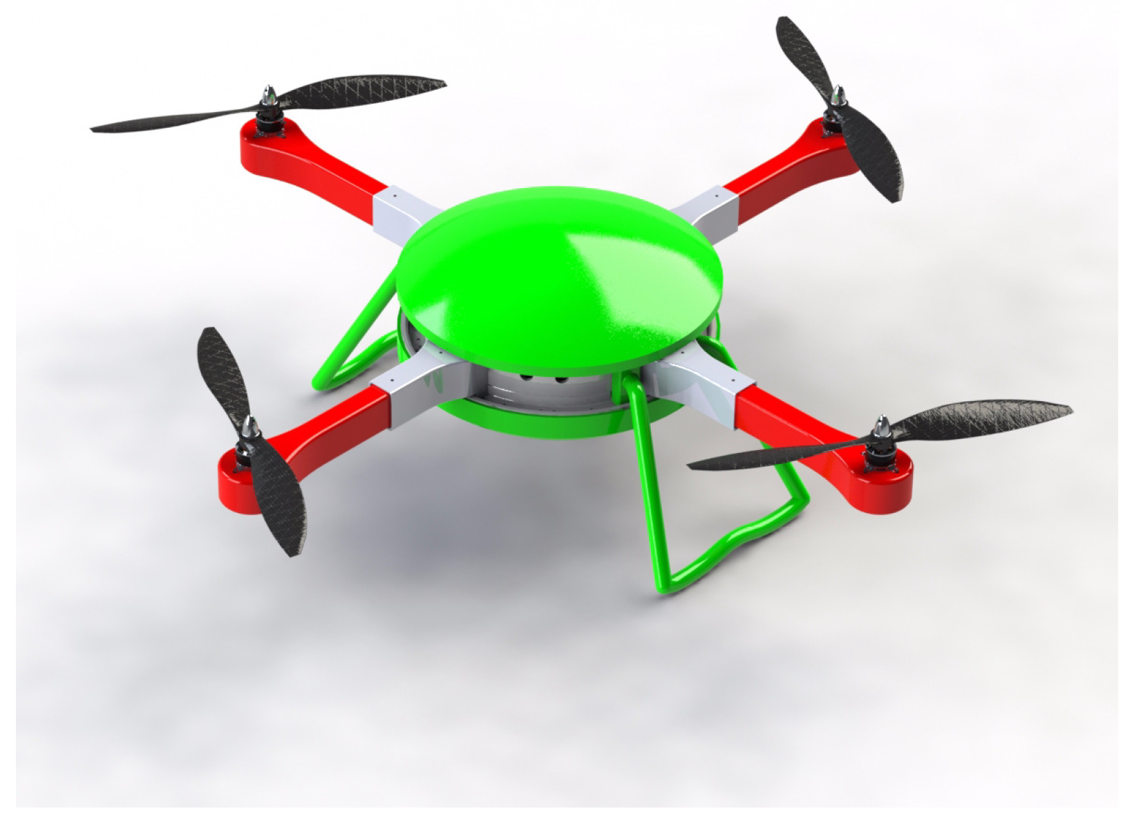
In order to emphasize the diffusion of this platform, Fused Deposition Modeling (FDM) has been chosen as the construction technique to allow anyone with a 3D desktop printer to construct a prototype in a fast and economical way [7]. Using a low-cost building technology, it is possible to build each part of the flying machine at home reducing the spare parts’ cost and the supply chain management; see the comparison with a drone factory such as Parrot or DJI. The model of part replacements and improvements on the main frame will be delivered as reported in [8]. A render of the prototype, which successfully flew for the first time on 4 July 2016, can be seen in Figure 1. PoliDrone is a multipurpose modular drone with adjustable arms produced via the FDM additive manufacturing process [9]. The combination of only eight basic constituent elements used in different ways and number allows 12 different configurations. These configurations are 3-, 4-, 6- and 8-arm configurations with the possibilities of single rotor, double rotor or system rotor + inflatable element per arm. This idea is completely new if compared with other modern drones proposed in [10,11,12,13].
The first PoliDrone prototype has been produced, via the 3D FDM printing process, using PLA (PolyLacticAcid) for all of the elements [9]. PLA is a green and recyclable material. It is quite easy to print. The main aim of the project is the construction of a second prototype with a total weight (including a pay load of 0.5 kg) less than 2 kg. In this way, we can take advantage of the facilities provided by the ENAC (Ente Nazionale Aviazione Civile or National Authority for Civil Aviation) regulation. In order to obtain this aim, three main steps must be followed. The first step is the definition of a new geometry for the prototype where some parts are redesigned. The second step is the use of a new material in combination with the FDM technique: ABS (Acrylonitrile Butadiene Styrene) in place of PLA. ABS is lighter than PLA (better specific properties), and it does not have deterioration of its properties through time (PLA has deterioration). However, the FDM printing process is not so easy if combined with the use of ABS [14,15]. The third step is the appropriate Finite Element (FE) analysis of the prototype and the relative structural optimization. In order to perform such an analysis, the ABS properties must be known. We know the properties of the ABS filament, but after the FDM process, such properties change and become unknown. We need these properties in order to perform a correct FE analysis. ABS has been chosen due to its good mechanical properties combined with a reduced weight. In order to design and optimize the primary structure of the multi-copter, knowing the applied loads, it is mandatory to have the material properties with a statistical level of confidence. This feature is necessary because during the extrusion process, there are several machine parameters that can influence the mechanical properties of the finished pieces [14]. Moreover, for a flying product, not only the mechanical properties are requested, but also the dimensional capabilities of the machine must be investigated in order to design the correct machine drawing, allowing perfect joints between different subparts [15].
It is important to notice that ABS can be polymerized in varying proportions and that the manufacturing process and machine precision can influence its properties. In general, three different directions of building are possible in the case of the FDM 3D printing process. For each building direction, the raster orientation can also be selected (e.g., / in our study cases). For these reasons, a complete characterization is necessary for each building direction. In order to have a first satisfactory ABS characterization, a possible and general work plan could be:
- Tensile characterization for building Direction 1 for the specimen production
- Compressive characterization for building Direction 1 for the specimen production
- Bending characterization for building Direction 1 for the specimen production
- Tensile characterization for building Direction 2 for the specimen production
- Compressive characterization for building Direction 2 for the specimen production
- Bending characterization for building Direction 2 for the specimen production
- Tensile characterization for building Direction 3 for the specimen production
- Compressive characterization for building Direction 3 for the specimen production
- Bending characterization for building Direction 3 for the specimen production
The tensile characterization for the first building direction has been performed by the same authors in [16]. Some preliminary information about the compressive characterization for the first building direction has already been proposed in [17]. The complete and exhaustive compressive test for ABS specimens built in Direction 1 is the topic of this new work. Interesting studies and characterization tests of structural elements including ABS and produced via additive manufacturing have been proposed in [18,19,20,21,22].
A capability study focused on the compression analysis of specimens built with a Sharebot NG 3D Printer will be presented. Furthermore, a capability analysis on the dimensional properties, which measures the dimensional characteristics of the same specimens, will also be performed. The proposed statistical theory is based on the the Six Sigma Process.
2. The Compression Test
The aim of this experimental campaign is to determine the compressive properties of ABS specimens produced with the FDM technique implemented in a home desktop Sharebot NG printer with a single extruder. The reference standard for the determination of the compressive properties of plastic materials (reinforced or not) is the ASTM D695 [23]. In the case of isotropic materials, at least five specimens must be tested. For this reason, nine specimens have been employed in the present test.
This standard proposes two types of specimen, depending on the properties to be determined. When compressive strength is desired, the specimens must have the form of a right cylinder or prism where the length is twice its principal width or diameter. However, when compressive elastic modulus and offset yield-stress data are investigated, the geometrical dimensions of the specimens are expressed in terms of the slenderness ratio. The slenderness ratio is defined as the ratio between the length of a column of uniform cross-section and its least radius of gyration (0.25-times the diameter for specimens of a uniform circular cross-section or 0.289-times the smaller cross-sectional dimension for specimens of a uniform rectangular cross-section). The proposed slenderness ratio should be in the range from 11:1 to 16:1. The second kind of specimen, with a rectangular section, has been chosen for the present study of the compressive properties. The reasons have been explained in Section 2.1.
2.1. Specimen Characteristics
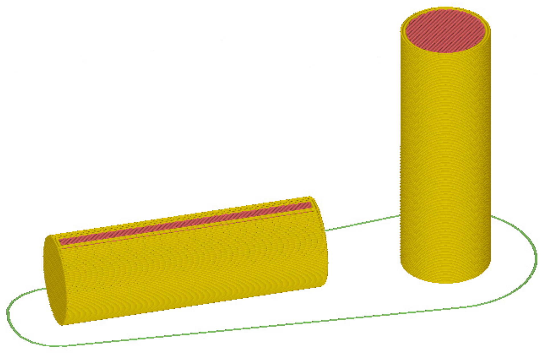
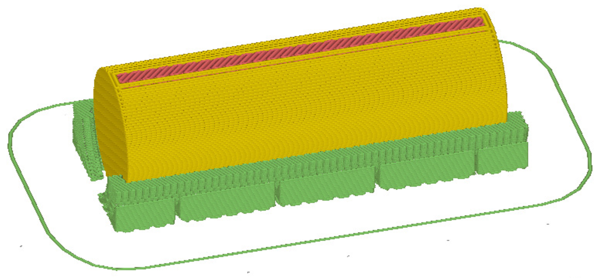
The specimen proposed by the standard evolves along a principal direction. Figure 2 shows two of the three different possible building directions. The first one would be preferable, being coherent with the direction chosen in the tensile test performed by the authors in [16]. However, the choice of a circular cross-section specimen creates some differences in the printing process, and the fused material needs an appropriate support. For this reason, a support material basin could be planned as shown in Figure 3.
For the first printing direction, the support material does not completely adhere, and the specimens separate from the printing floor. For the second building direction, there are some difficulties, such as the small contact section between the specimen and the floor and the presence of high vibrations. These vibrations induce the separation of some specimens during the printing process. For all of these reasons, square cross-section specimens have been chosen here. The contact area of a square section is greater than that of a circle section with the same principal dimensions. Therefore, this type of specimen provides a greater adhesion. The dimensions were set to have a slenderness ratio, close to the lower values (from 11:1 to 16:1) proposed in the previous section, which avoids similar issues to the ones previously mentioned. The use of a square cross-section allows the use of the same printing direction employed for the tensile ABS characterization proposed in the work [16]; this direction and the specimen are indicated in Figure 4.
2.2. Printing Parameters
The mechanical properties of 3D printed pieces are influenced by several printing parameters. These values must be chosen before generating the file containing the instructions to be followed by the printer. In the case of specimens for compression tests, Ahn et al. [24] examined only the building direction as a printing parameter, determining that a specimen with a building direction transverse to the compression direction would have shown a higher compressive strength. Since the influence of the other parameters was not investigated in the literature, it was chosen to set the printing parameters consistently with the tensile test already performed in [16]. Hereinafter, these parameters will be presented, together with their numerical values chosen by the authors. A specific explanation for each of these parameters can be found in [16]:
- Bead/Raster width: It is related to the nozzle gap as it represents the transverse dimension of the extruded bead. The nozzle size of the Sarebot NG is 0.35 mm [25]. Therefore, this fixed value was set.
- Perimeters: It represents the peripheral beads to be deposited. Two perimeter walls were used in the present work.
- Air gap: It is used to set the distance between two adjacent deposited beads in order to specify the internal infill density, which was set to 100%. The aim is to obtain solid specimens without overlapping beads.
- Bed temperature: The print plane was heated to 90 °C to prevent the deformation of specimens after a quick cooling.
- Build temperature: ABS is commonly extruded in a temperature range between 220 °C and 250 °C. Therefore, a nozzle temperature of 245 °C was set here.
- Raster orientation/angle: When the fill-pattern is rectilinear, it indicates the orientation angle of the filling beads. Crisscross specimens were here printed with a lamination sequence of 45°/°.
- Layer height: it measures the vertical dimension of each extruded bead. It was set to 0.2 mm.
2.3. Test Setup
Before starting the experimental campaign, it is compulsory to measure the width and thickness of each specimen to the nearest 0.01 mm, at several points along its length, recording the minimum value of the cross-sectional area. The length of each specimen must be also measured. Beyond the specific reasons for which such measurements are made, they can be useful in determining some “best practices” for the design phase to ensure the dimensional compatibility of the pieces to be printed, taking into account the errors introduced in the printing process. The measurements shown in Table 1 were made using a Burg Wachter PRECISE PS 7215 digital caliper, whose measuring range and accuracy are 150 mm and 0.01 mm, respectively [26]. Thickness and width values refer to the smallest section. The first specimen has been discarded because it has not given satisfactory results.
An MTS QTEST 10 testing machine [27] (see the example in Figure 5 proposed for the tensile test) was used; each specimen was placed between an upper and a lower planar support taking care of the fact that the surfaces of the compression tools were parallel with the end surfaces of the specimen and aligning the center line of its long axis with the center line of the machine. As the common testing machines can be controlled in speed or in load, the standard requires that the test takes place in speed control, with a constant speed of the movable support of 1.3 mm/min. It is also suggested to increase the speed after the yield point, but only if the machine has a weighing system with rapid response and the material is ductile. However, it was preferred to maintain constant the load application speed for simplicity. In the specific case of this testing machine, the absolute position is that of the upper support.
3. Numerical Analysis
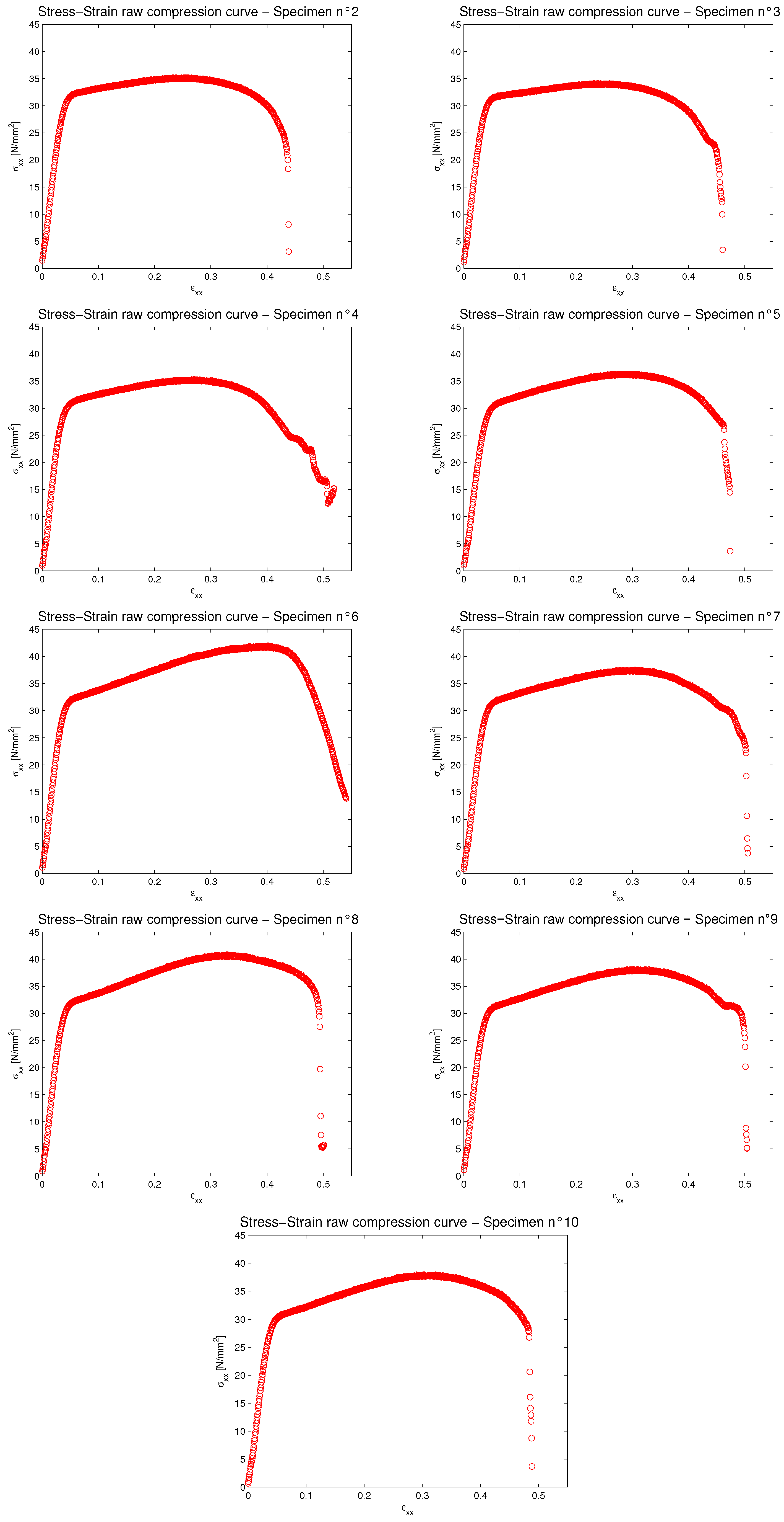
The raw stress-strain curves for the nine selected specimens are shown in Figure 6 where the compression behavior of each specimen is provided.
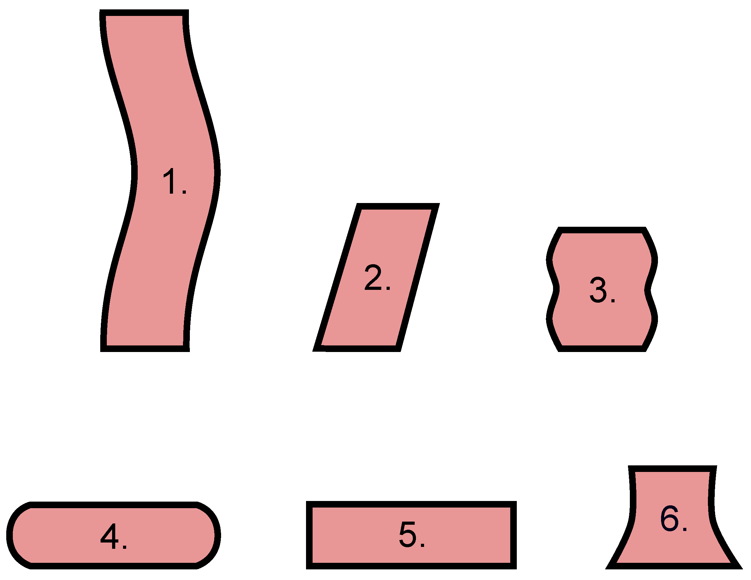
All of the proposed specimens show the common linear-elastic region, followed by a non-linear zone. Until about the proportional limit, the specimens show no macroscopically appreciable deformations. Subsequently, a first bulge of the central section appeared, followed by a progressive buckling of the specimen. Figure 7 shows the different modes of deformation that can occur in a compression test.
- typical buckling mode: it happens when the ratio between the sample length and its width exceeds five;
- shearing mode: it may happen when the ratio between the sample length and its width is about five;
- double barreling mode: it may happen when the ratio between the sample length and its width exceeds two and friction is present at the contact surfaces;
- barreling mode: it happens when the ratio between the sample length and its width is less than two;
- homogenous compression mode: it happens when the ratio between the sample length and its width is between 2.0 and 1.5;
- compression instability mode.
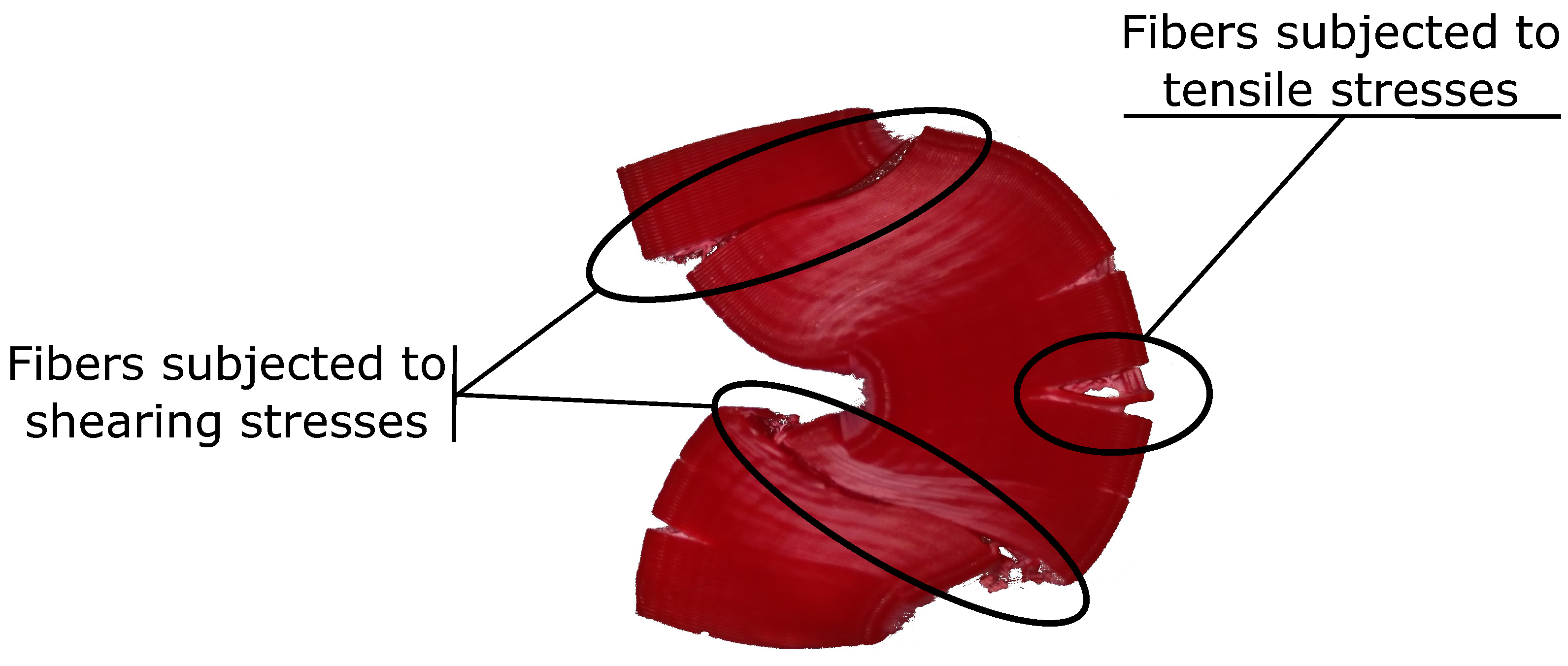
The tested specimens have a slenderness ratio of 12 (as will be calculated in Section 3.2). The ratio between the length and the width is 3.5. For this type of specimen, the standard [23] does not provide for the use of a support jig to avoid the buckling of the specimen. Even if the ratio between the length and the width is 3.5, all of the specimens, after an initial deformation, which can be assumed as Mode 4, moved to the typical buckling mode. After reaching a maximum stress value in buckling mode, all of the specimens started to break up into zones with fibers subjected to tensile and shearing stresses. Figure 8 details the deformation evolution during the compression test. Figure 9 shows a typical broken specimen where fibers subjected to tensile and shearing stresses are mentioned.
3.1. Post Processing According to ASTM 695
Each datum collected from the compression test has been treated according to ASTM 695 (technically equivalent to the ISO 604) [23] in absence of a specific normative for FDM 3D printed objects. ASTM 695 norms collect the standard methods of test for the compressive properties of rigid plastics, un-reinforced or reinforced, including also composites, when loaded in compression at low uniform rates. Each of the stress-strain curves shows in the linear-elastic region a horizontal tangent point, spacing two sections with slightly different slopes. This toe region is an artifact caused by the take up of slack and alignment or seating of the specimen. As it does not represent a property of the material, it was compensated drawing a continuation of the linear region of the curve until the zero-stress is reached and considering the intersection of this straight line with the strain axis as the correct zero strain point. The compressive properties that can be determined by this experimental campaign are:
- Compressive modulus of elasticity: The coefficients of the linear regressions based on point-by-point increasing ranges of values were averaged. This procedure had as the starting point the one next to the graph change of slope and as the ending point the one at which the new regression coefficient differed by more than 5% from the averaged one.
- Compressive proportional limit: From the previously found modulus of elasticity, it was possible to identify the stress value, which differed by more than 5% from the expected value; this was conventionally identified as the proportional limit
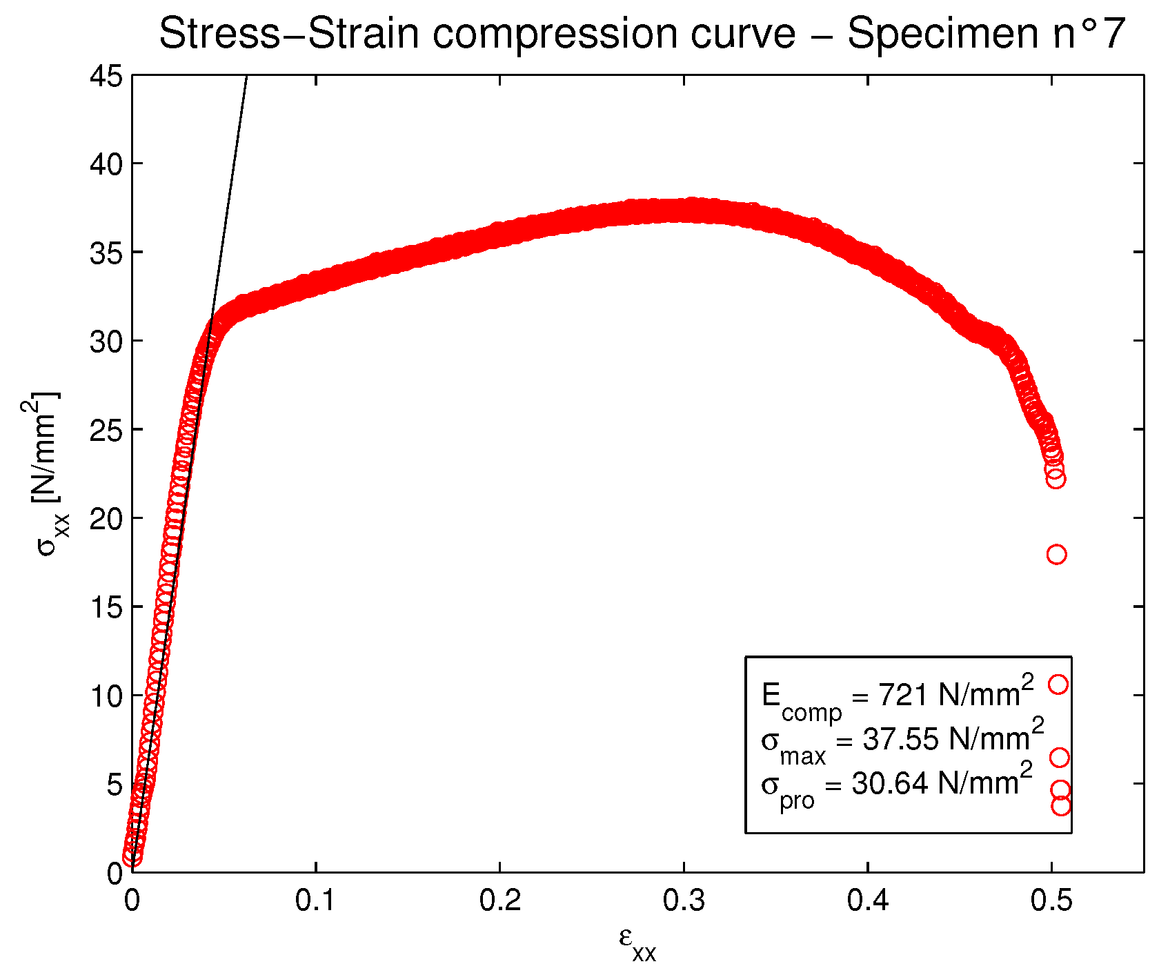
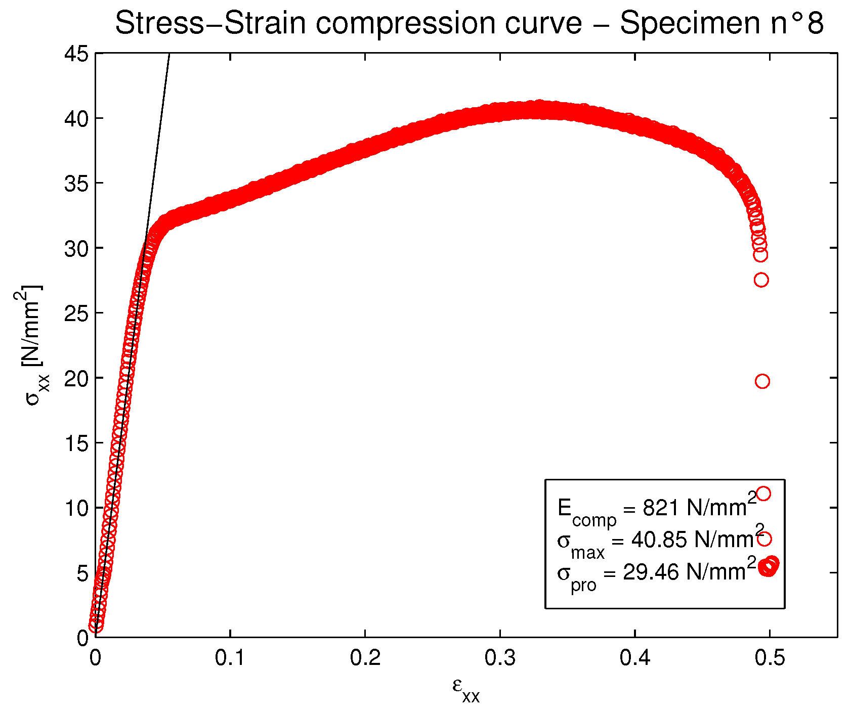
- Maximum compressive stress: It was calculated by dividing the maximum load by the minimum cross-sectional area value. However, as all of the specimens suffered buckling, it is not advisable to take account of these values as compressive strength, and it will be necessary to repeat the test with more stubby specimens in accordance with the standard. The results are reported in any case to be thorough.
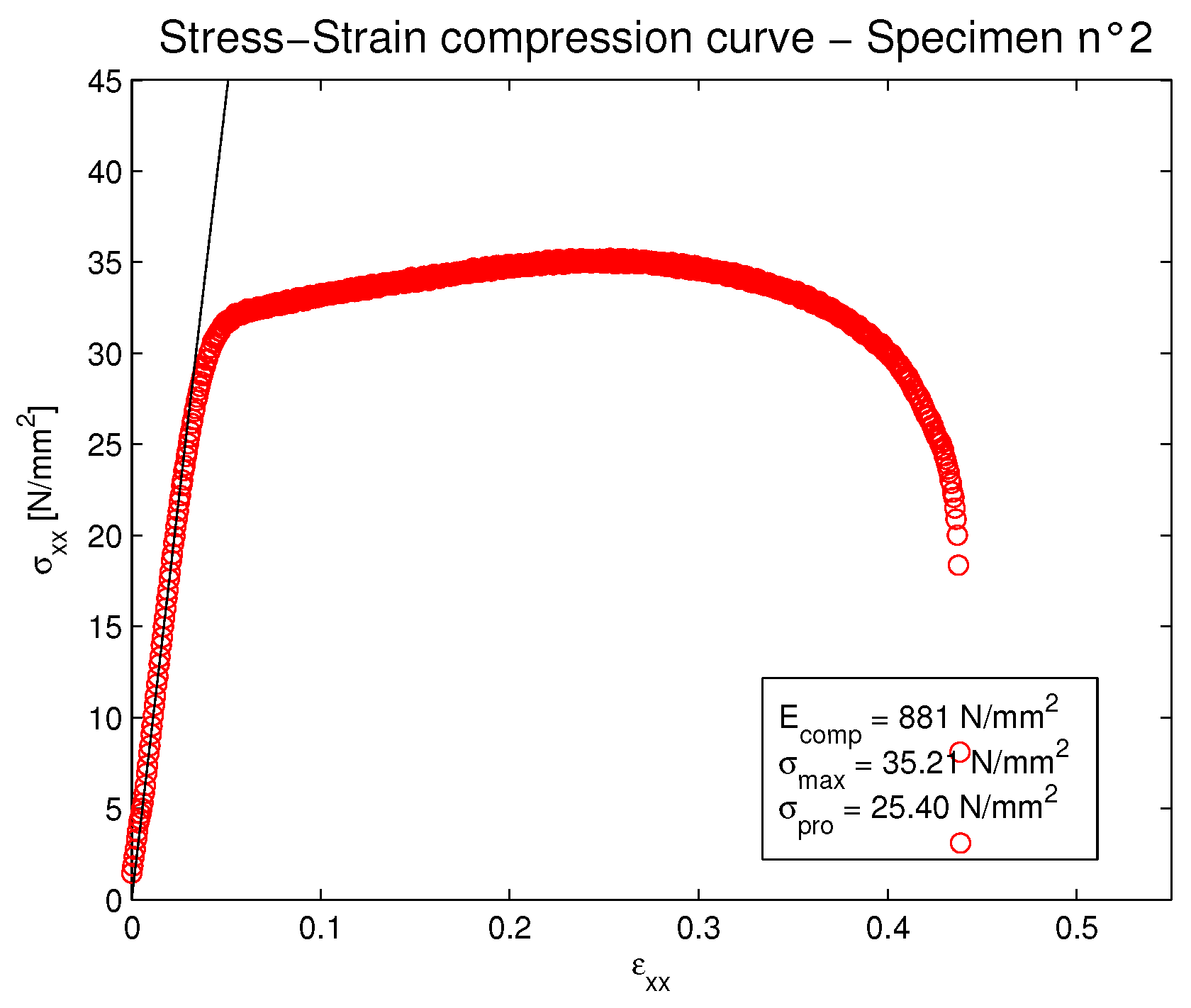
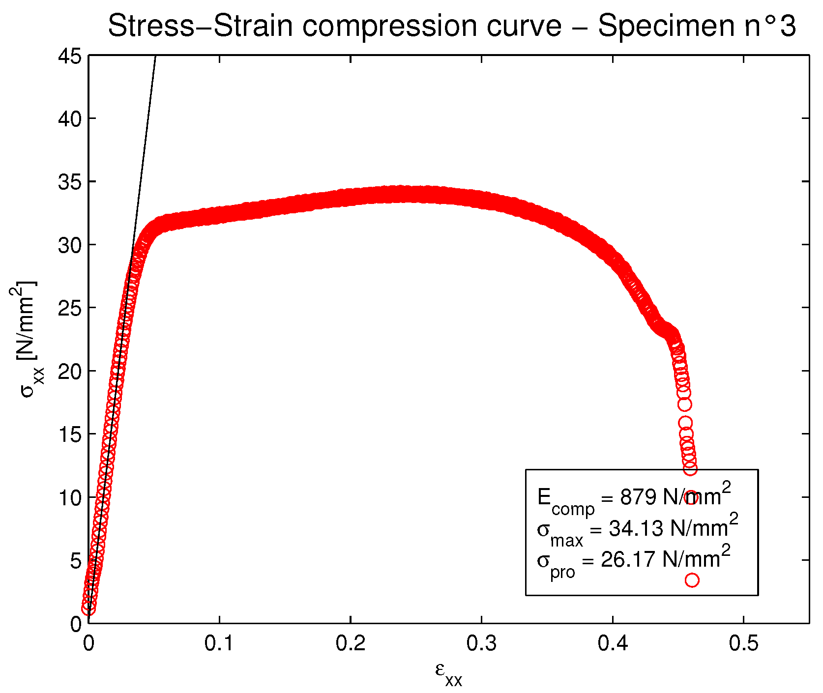
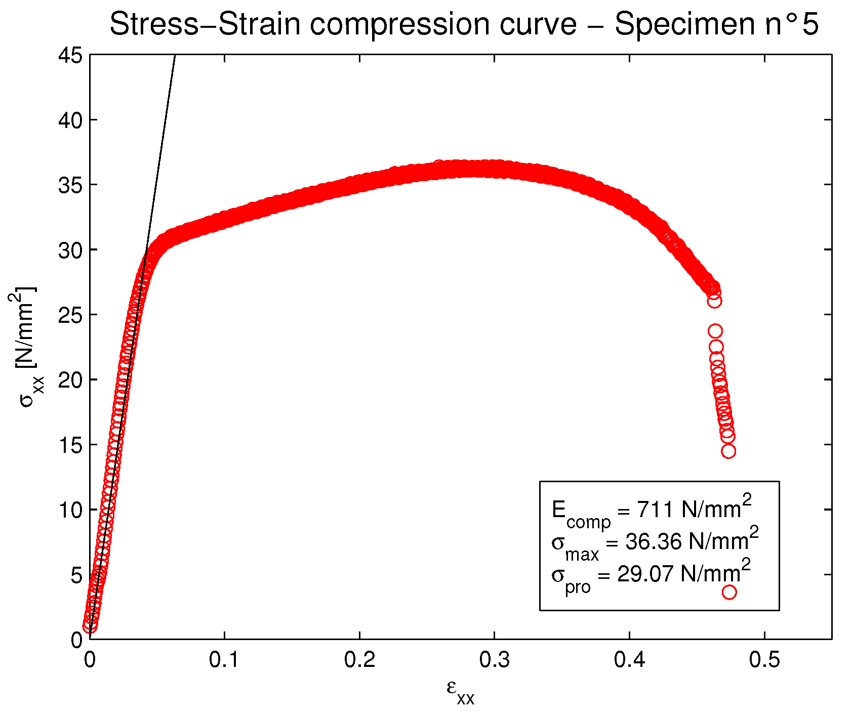
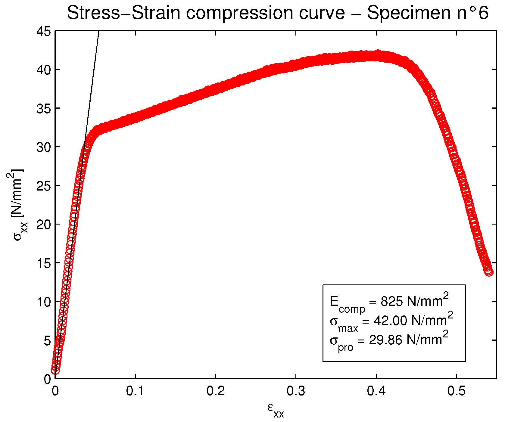
The application of corrections to the the linear portion of the stress-strain curve was not necessary in this work. The plots for each of the nine specimens are presented in Figure 10, Figure 11, Figure 12, Figure 13, Figure 14, Figure 15, Figure 16, Figure 17 and Figure 18. Table 2 gives the collected results already shown in Figure 10, Figure 11, Figure 12, Figure 13, Figure 14, Figure 15, Figure 16, Figure 17 and Figure 18.
3.2. Compression Critical Load
The critical load is defined as the maximum load that a column can bear while staying straight. As before buckling, the specimens show no macroscopic deformations, it was interesting to investigate the theoretical value of the compression critical load to verify that it is higher than the proportional limit. As the slenderness ratio of a column increases, the critical load first follows the parabolic Johnson formula, then the hyperbolic Euler one [30]; the transition point can be expressed in the form of the slenderness ratio, imposing the tangency between the two curves [30]. The slenderness ratio can be calculated as:
where is the effective length, the radius of gyration, E the tensile elastic modulus and the tensile maximum stress (it is obtained from past authors’ work [16] where it is clear how the maximum tensile stress is very close to the tensile yield stress; this last stress has not been calculated in [16]).
The specimens will be analyzed as approximating pinned-pinned columns. Therefore, the effective length coincides with the real one, making A coincide with the slenderness ratio defined at the beginning. Taking into account the ABS tensile elastic modulus and the maximum stress found in [16], this formula leads to a slenderness ratio of . As the specimens’ slenderness ratio (calculated as ) is 12, they can be interpreted as intermediate length columns, so the Johnson parabolic transition formula should be used:
This calculation, using a maximum tensile stress of in place of the yield stress (see the past authors’ work [16]), gives a critical stress of , which is slightly higher than the proportional limit and lower than the compressive strength. This feature means that all specimens collapsed for buckling reasons. However, results for elastic modulus E and proportional limit are valid. On the contrary, new specimens with a different A value must be produced to obtain a higher value for the critical stress in order to correctly identify the maximum compressive stress. In Equations (1) and (2), the employed Young modulus is the mean value obtained in the tensile test performed in [16]. This choice has been made because it is more conservative for the calculation of . The tensile test in [16] proposed a proportional limit equal to (mean value).
3.3. Statistical Analysis
As already done for the tensile properties determined in [16], the mechanical and dimensional experimental values are here evaluated for compressive tests setting up a capability analysis. Since the mechanical properties and the geometrical values (in the sense of the printing deviations from the nominal values) are determined, the capability analysis is implemented to determine the upper and lower limits of these quantities, which can limit in a statistically stable way the experimental values.
As a precondition, it is necessary to verify if the investigated quantities could be approximated with a normal distribution. The Anderson–Darling hypothesis test [31,32] measures how well the data follow a particular distribution considering the values of two indices, which are the AD (Anderson–Darling statistic) and the p-value. For a specific set of data and a number of different distributions, the better fit is obtained for the smaller value of AD. The probability index should be as high as possible. A reference value of 0.05 or 0.1 usually allows excluding or considering a certain distribution.
A goodness of fit test is set up for all of the experimental quantities shown in Table 1 and Table 2. These results are given in Table 3 and Table 4. It is necessary to verify if the Anderson–Darling statistic of a certain distribution was substantially smaller than the ones of the others and that, simultaneously, the correspondent p-value is higher than the reference value. The normal distribution does not always seem to be the best fit. However, both the indices allow its use. This analysis is discussed in detail in the next section.
4. Results
This section proposes the results for the capability analysis. Such an analysis has been performed for the three investigated mechanical properties and for the dimensional characteristics, including also the weight of the produced specimens.
4.1. Capability Analysis for Mechanical Properties
In this section, the mechanical properties are investigated. The quantities which are taken into account are those presented in Section 3.1: the compression elastic modulus (E), the compression proportional limit () and the compression strength (). The sample was composed by 10 specimens, but the first one was used as a sacrificial specimen to understand the machine operation. Therefore, the experimental values of the nine employed specimens are reported in Table 2. The analysis is carried out by means of the control chart, the probability plot and the capability analysis, which are proposed for each quantity.
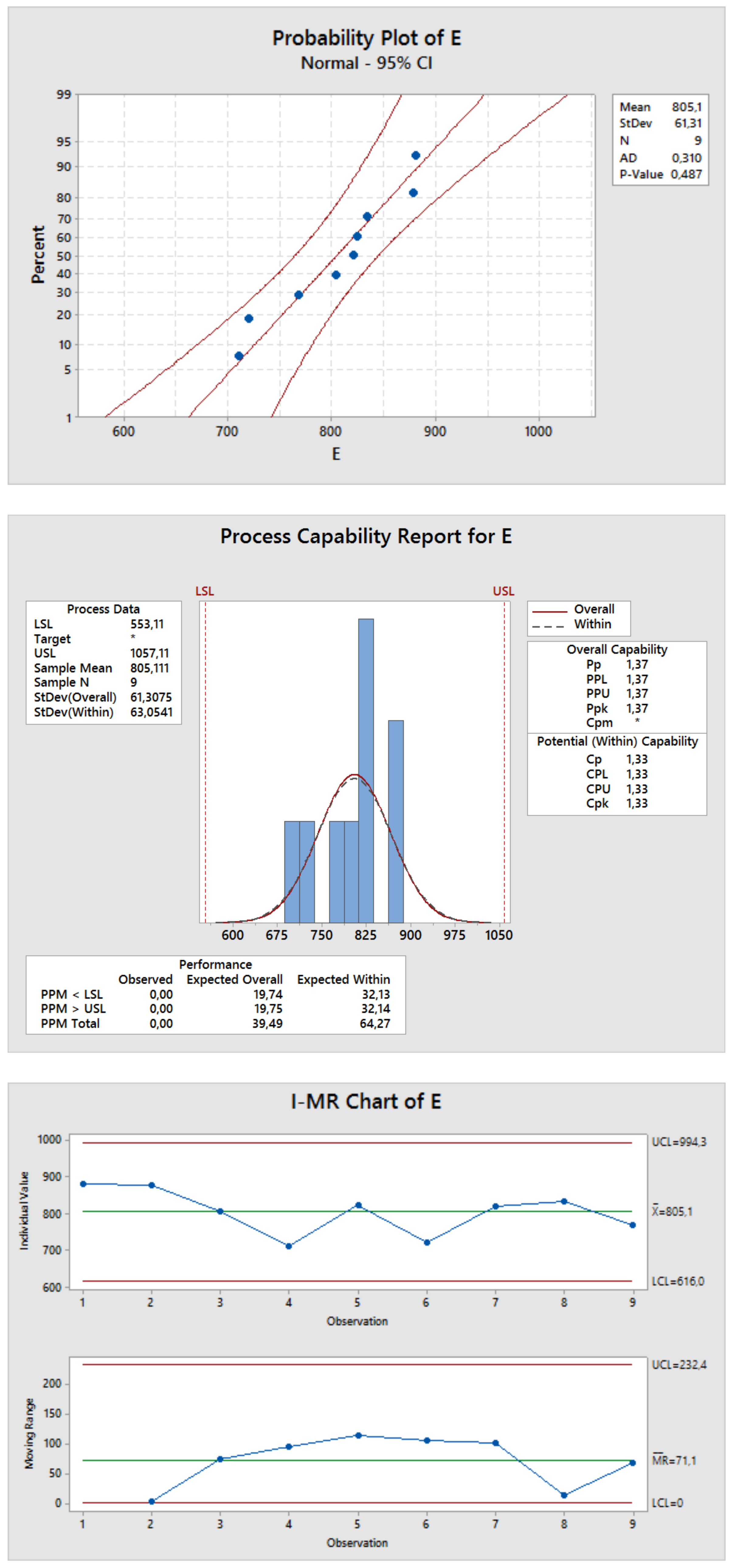
The first line of Table 2 shows the experimental collected values for the Young modulus E. The probability plot in Figure 19 shows that the average value of the overall sample is equal to , and the standard deviation is 61.31. The Anderson–Darling statistic value is equal to 0.310, which is not the smallest one among the considered distributions. However, being the p-value equal to 0.487, it is considerably higher than the threshold one (see Table 3). Therefore, the normal distribution can be considered a good fit for this set of data. Indeed, the data seem to follow approximately a straight line. The lower limit is , and the upper limit is . To identify the upper and lower limits delimiting in a statistically stable way the percentage corresponding to the Sigma Level 4, a P (Process Performance Adjusted for Process Shift index) equal to 1.33 was imposed; this would lead to a more conservative approach as it takes into account the long term variability, generally higher than the short one. However, as may happen while working with a small data sample size, P appeared to be lower than the corresponding C (Process Capability Adjusted for Process Shift index). Therefore, in this case, a C equal to 1.33 was imposed. This feature results in a lower limit equal to ; at least 99.38% of the specimens will have a higher compression modulus of elasticity. The I-MR (Individuals (I) chart and Moving Range (MR) chart) chart presented in Figure 19 shows that the process is globally stable and performs inside of the limits of acceptance of the Sigma Level 4.
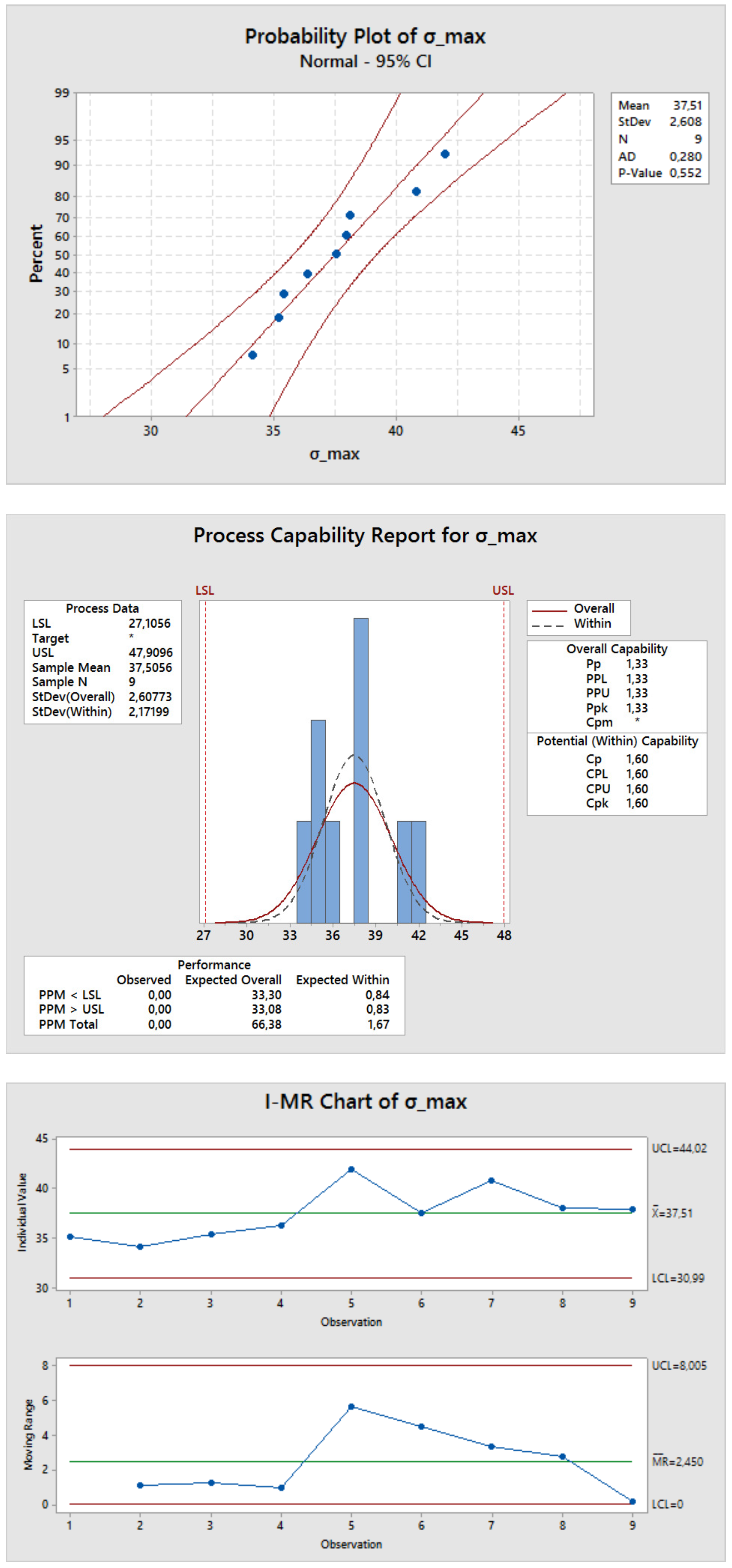
The experimental collected values for the compressive stress at rupture are given in the second line of Table 2. The overall sample mean is 37.51 , while the standard deviation is 2.608. From the probability plot in Figure 20, it can be deduced that the normal distribution can approximate this set of data well, as the Anderson–Darling statistic is 0.280 and the p-value is 0.552 (see Table 3). The capability report shows that the boundary limits for a P index equal to 1.33 are 27.1056 MPa and 47.9096 MPa. The graph is quite symmetrical, although the left part is more populated. This capability analysis has been proposed anyway even if the critical load is smaller than the compression stress at rupture . This study has been reported only to be thorough.
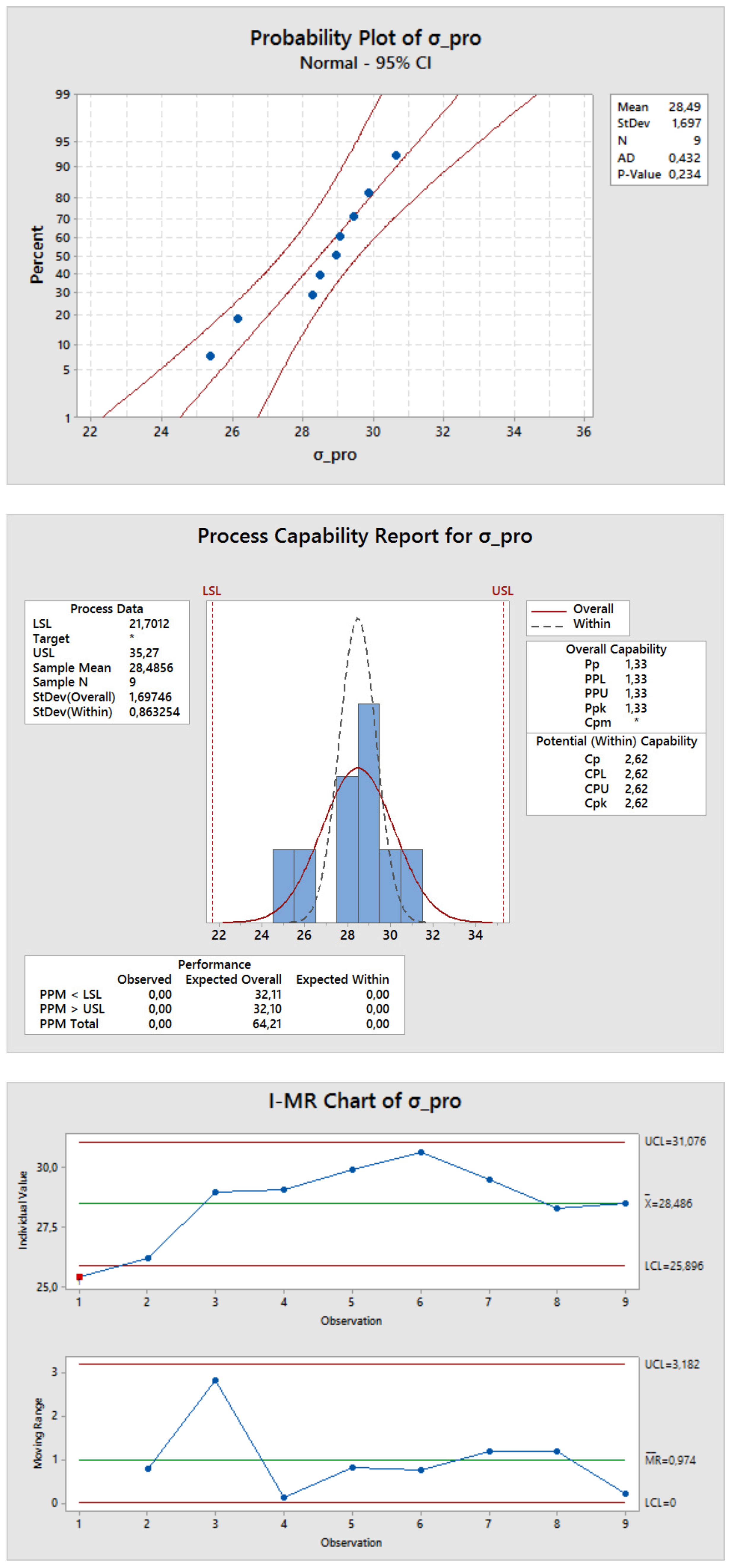
The compressive proportional limit is the last investigated mechanical characteristic. The experimentally-collected values are shown in the third line of Table 2. As can be seen in the probability plot of Figure 21, the data seem to follow a straight line, except for the the two smaller values. Indeed the Anderson–Darling statistic and the p-value suggest that the normal distribution approximates the difficulties of this dataset (see Table 3). The process capability report in Figure 21 underlines an important variability of this quantity, characterized by an average value of 28.49 MPa and a standard deviation of 1.697. The boundary limits were identified in 21.7012 MPa and 35.27 MPa imposing a Ppk index (Process Performance Adjusted for Process Shift index) equal to 1.33. The last graph of Figure 21 shows that, except for the first two specimens, the process is stable and inside of the boundaries.
4.2. Capability Analysis for Dimensional Characteristics
In this section, the dimensional characteristics are investigated. Four quantities are taken into account: the X dimension and the Y dimension of the smallest section, the overall length and the weight (which shows the variability of the amount of extruded material). The sample was composed by nine specimens; all of the experimental values are given in Table 1. The analysis is carried out by means of the control chart, the probability plot and the capability analysis, which are presented for each of the four considered quantities.
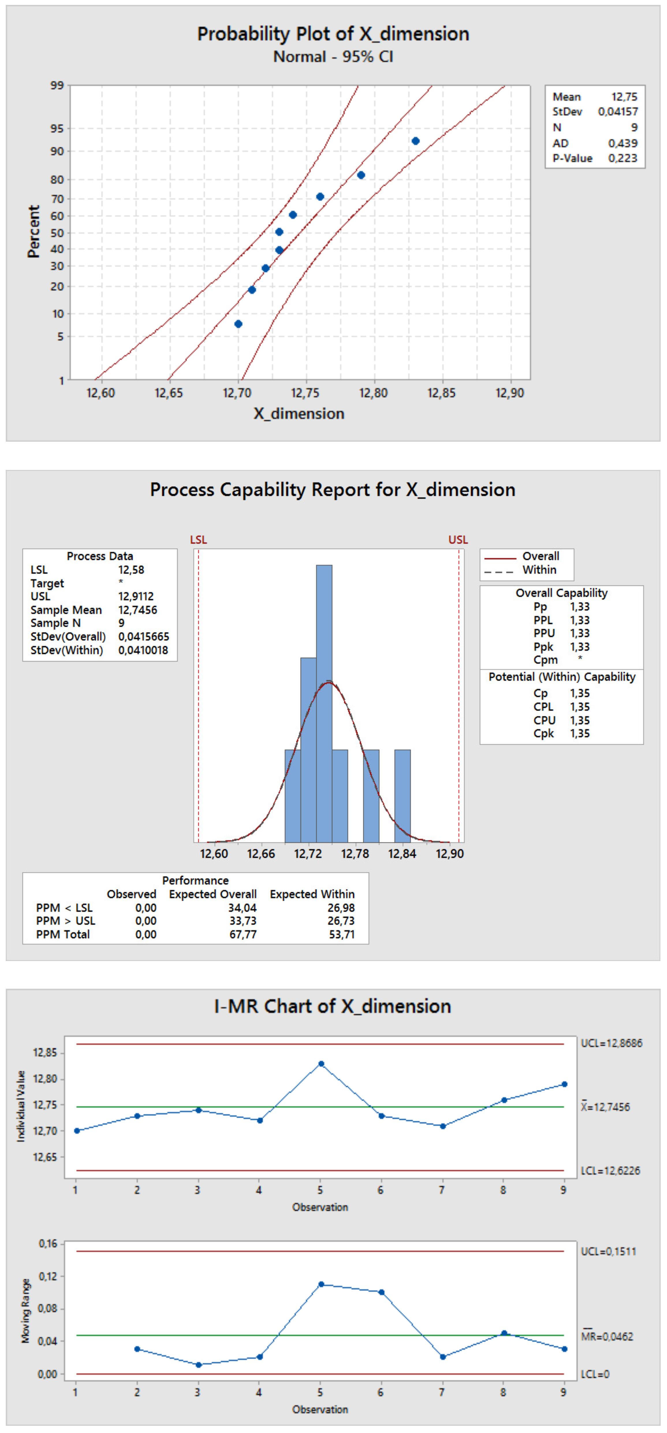
The nominal value of the X dimension is 12.70 mm. The average real value is 12.75 mm, with a standard deviation of 0.04157. From the probability plot of Figure 22, it can be seen that the measurements seem to be shifted towards values higher than the nominal value. As the Anderson–Darling statistic is not so low and the p-value is 0.223, the normal distribution shows some difficulties in approximating this data distribution (see Table 4). However, the average percentage error on the X axis is just 0.4%, and this information can be introduced as a re-scaling factor. The lower and upper limits, delimiting the specimens’ percentage corresponding to the Sigma Level 4, were identified, respectively, imposing a P equal to 1.33, in 12.58 mm and 12.9112 mm. This approach takes into account the long-term variability, and it is, therefore, conservative, as it leads to a C equal to 1.35.
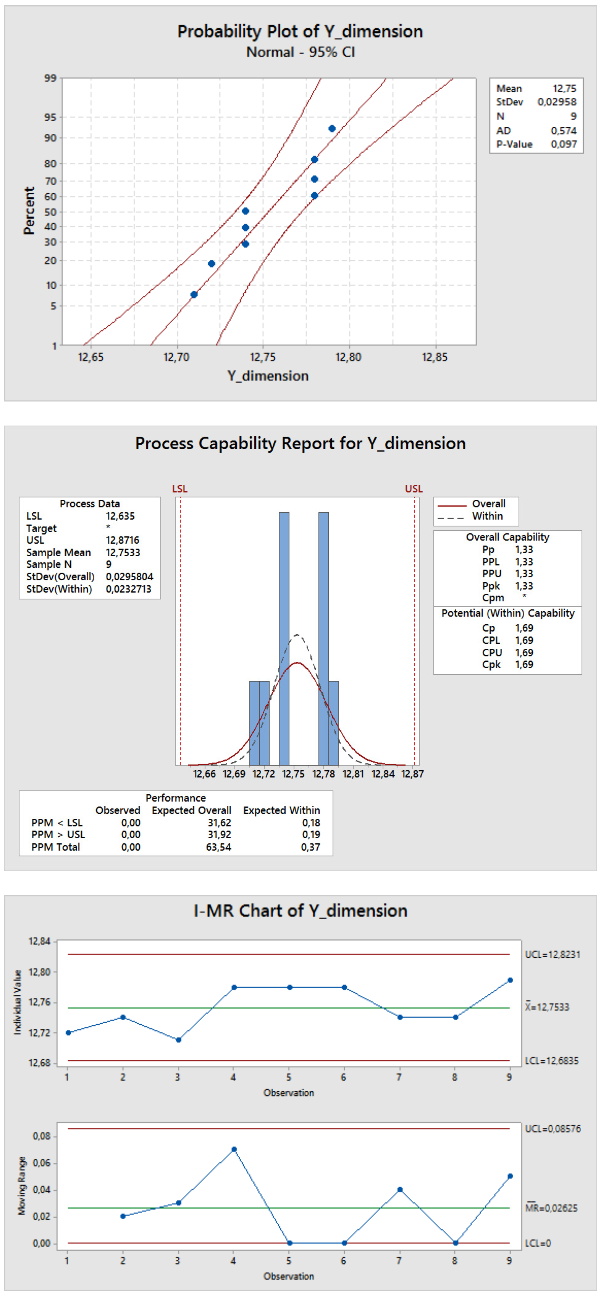
The Y dimension parameter allows evaluating the printer’s behavior along the Y axis. As for the X dimension, the nominal value is 12.70 mm. The average value is also 12.75 mm, as can be seen in the probability plot of Figure 23. This figure shows that also in this direction the printer manifests an average percentage error of 0.4%. However, the collected values do not follow a normal distribution, as can be seen from the extremely low p-value (see Table 4). Furthermore, the largest number of measures tends to be focused on values of 12.74 mm and 12.78 mm. It is therefore advisable to repeat the study on this axis, to better understand this behavior, trying to identify the possible existence of external effects. A P value (Process Performance Adjusted for Process Shift index) of 1.33 was imposed, leading to a lower specification limit of 12.635 mm and an upper specification limit of 12.8716 mm. The capability histogram in Figure 23 shows an equally-spaced distribution. The in-plane performance of the printer seems to have the same percentage deviations from the nominal ones. However, further analysis should be carried out to identify the sources of the random behavior manifested in the Y dimension before taking into account a scale factor when the printing instructions are sent to the printer. The printer’s behavior in the printing peripheral areas should also be deepened, as the specimens, having small dimensions, were always printed in the central area.
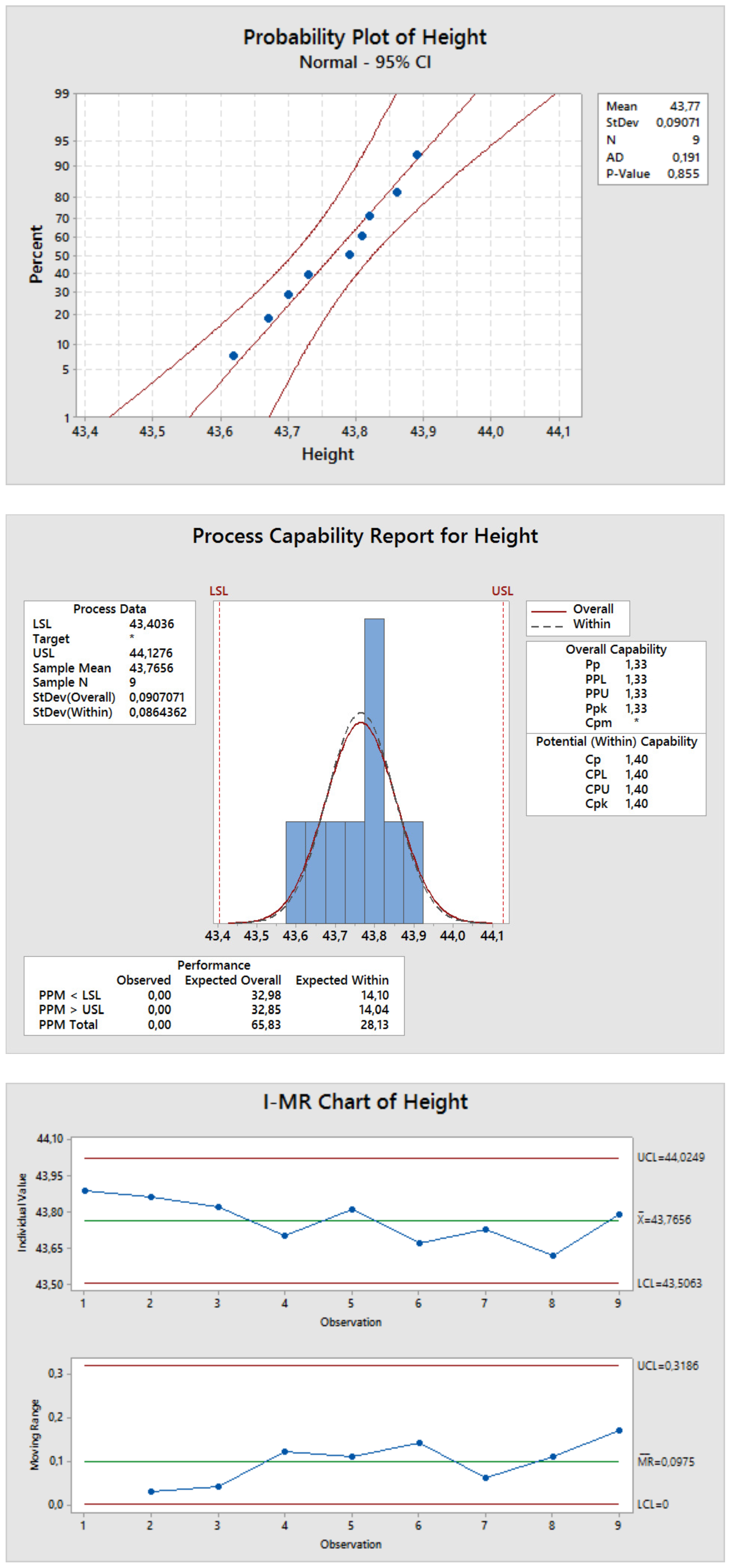
The length of the specimens allows evaluating the out-of-plane behavior of the printer. The design value is 44.00 mm. The probability plot of Figure 24 shows that the real dimension is always smaller than the nominal one. The average real value is 43.77 mm with a standard deviation of 0.09071. In this case, the process seems to be stable and controlled, as the Anderson–Darling statistic is significantly low, and the p-value is 0.855 (see Table 4). The capability histogram reveals that the process is well centered on the average value; indeed a lower specification limit of 43.4036 mm and an upper one of 44.1276 mm lead to similar P and C indices, respectively 1.33 and 1.40. The average error introduced in the printing process can be evaluated in −0.5%. This information is stable, and it can be used as a re-scaling factor with confidence. However, also in this case, the printer’s behavior in printing peripheral areas should be studied.
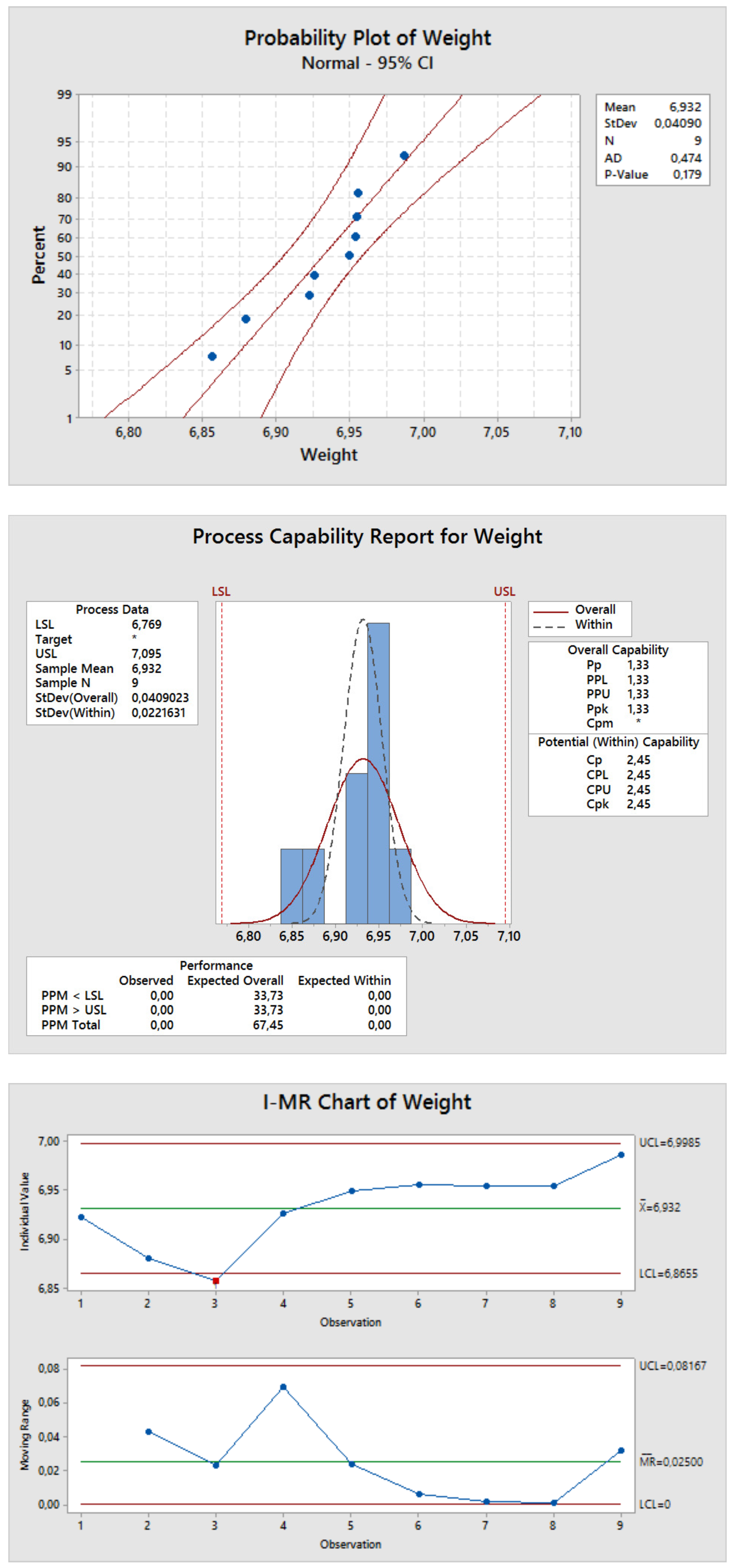
The capability analysis on specimens’ weight is made to determine how the amount of extruded material varies during the process. The specimen’s volume was evaluated through its nominal dimensions; it should be equal to 7096.76 mm. The density of ABS filament declared by the vendor is 0.0011 g/mm. Therefore, a weight of 7.806 g is expected. Values shown in the last line of Table 1 indicate that the printer underestimated the amount of material to be extruded; indeed an average value of 6.932 g was found. This is consistent with what was found in the previous authors’ work about the tensile characterization of ABS [16]. The behavior reported in Figure 25 is quite random, as the values do not seem to follow the straight line. Therefore, the Anderson–Darling statistic is low, and the p-value is just over the reference value (see Table 4). However, the lower limit is 6.769 g, and the upper limit is 7.095 g.
5. Conclusions and Further Developments
The tensile properties of ABS specimens, printed with a desktop 3D printer, were studied in [16]. In order to fully characterize the mechanical properties of 3D-printed ABS, further analyses are necessary. One of these further analyses, here proposed, is the study of the compressive properties. A capability analysis, to evaluate if the 3D printing process is adequately stable for the self-production of flying components, has also been performed. A Sigma Level of 4 is chosen, so the lower limits for compressive elastic modulus, proportional limit and maximum stress were identified in 553.11 MPa, 21.7012 MPa and 27.1056 MPa, respectively. The found proportional limit and maximus stress are consistent with the compressive strength found in [24]. Being sufficiently conservative, these values can be used with confidence as input for a structural analysis. It is interesting to note that the critical load value is consistent with the experimental evidence. As stated before, the specimen shows some macroscopically appreciable deformation at a load level higher than the proportional limit. The ideal critical load resulted in being higher than the proportional limit. It is advisable to repeat the compression test with more stocky specimens (in order to avoid the buckling mode), to correctly evaluate the compressive maximum stress here wrongly calculated as 27.1056 MPa. This experimental campaign can be completed with the bending test and with the repetition of tensile, compressive and bending tests for the other two printing directions.
Acknowledgments
The authors thank Raffaella Sesana for the assistance with the testing of the specimens and for advice that greatly improved the manuscript. We would also like to give our gratitude to all of the members of the PoliDrone team for their support and constant work.
Author Contributions
All authors contributed equally to this work.
Conflicts of Interest
The authors declare no conflict of interest.
References
- Wright, D. Drones: Regulatory challenges to an incipient industry. Comput. Law Secur. Rev. 2014, 30, 226–229. [Google Scholar] [CrossRef]
- Clarke, R.; Moses, L.B. The regulation of civilian drones’ impacts on public safety. Comput. Law Secur. Rev. 2014, 30, 263–285. [Google Scholar] [CrossRef]
- Clarke, R. The regulation of civilian drones’ impacts on behavioural privacy. Comput. Law Secur. Rev. 2014, 30, 286–305. [Google Scholar] [CrossRef]
- ENAC Regulation, Remotely Piloted Aerial Vehicles. Available online: https://www.enac.gov.it/repository/ContentManagement/information/N122671512/Reg_APR_Ed202_2.pdf (accessed on 26 July 2015).
- Montgomery, A. The Drone Economy Moves Beyond Science Fiction. Available online: https://www.forbes.com/sites/mikemontgomery/2015/11/05/the-drone-economy-moves-beyond-science-fiction/#3828b9022aa3 (accessed on 4 May 2017).
- Brischetto, S.; Ciano, A.; Raviola, A. A Multipurpose Modular Drone with Adjustable Arms. Patent Temporary Number 102015000069620, 5 November 2015. [Google Scholar]
- Ferro, C.G.; Grassi, R.; Seclì, C.; Maggiore, P. Additive Manufacturing Offers New Opportunities in UAV Research. Procedia CIRP 2015, 41, 1004–1010. [Google Scholar] [CrossRef]
- Khajavi, S.H.; Partanen, J.; Holmstro, J. Additive manufacturing in the spare parts supply chain. Comput. Ind. 2014, 65, 50–63. [Google Scholar] [CrossRef]
- Brischetto, S.; Ciano, A.; Ferro, C.G. A multipurpose modular drone with adjustable arms produced via the FDM additive manufacturing process. Curved Layer. Struct. 2016, 3, 202–213. [Google Scholar] [CrossRef]
- Rossi, G.; MORETTI, S.; CASAGLI, N. An Improved Drone Structure. Patent WO2015036907A1, 19 March 2015. [Google Scholar]
- Choe, J.P. The Rotor Arm Device of Multi-Rotor Type Drone. Patent KR101456035B1, 4 November 2014. [Google Scholar]
- Guilhot-Gaudeffroy, M. Gyroptere a Securite Renforcee. Patent WO2004113166A1, 29 December 2014. [Google Scholar]
- Desaulniers, J.-M. Amphibious Gyropendular Drone for Use in e.g., Defense Application, has Safety Device Arranged in Periphery of Propulsion Device for Assuring Floatability of Drone, and Upper Propulsion Device for Maintaining Drone in Air During Levitation. Patent FR2937306A1, 23 April 2010. [Google Scholar]
- Krache, R.; Debbah, I. Some mechanical and thermal properties of PC/ABS blends. Mater. Sci. Appl. 2011, 2, 404–410. [Google Scholar] [CrossRef]
- Nunez, P.J.; Rivas, A.; Garcia-Plaza, E.; Beamud, E.; Sanz-Lobera, A. Dimensional and surface texture characterization in fused deposition modelling (FDM) with ABS plus. Procedia Eng. 2015, 132, 856–863. [Google Scholar] [CrossRef]
- Ferro, C.G.; Brischetto, S.; Torre, R.; Maggiore, P. Characterisation of ABS specimens produced via the 3D printing technology for drone structural components. Curved Layer. Struct. 2016, 3, 172–188. [Google Scholar]
- Brischetto, S.; Ferro, C.G.; Torre, R.; Maggiore, P. Tensile and compression characterization of 3D printed ABS specimens for UAV applications. In Proceedings of the 3rd International Conference on Mechanical Properties of Materials (ICMPM 2016), Venice, Italy, 14–17 December 2016. [Google Scholar]
- Bellini, A.; Guceri, S. Mechanical characterization of parts fabricated using fused deposition modeling. Rapid Prototyp. J. 2003, 9, 252–264. [Google Scholar] [CrossRef]
- Anitha, R.; Arunachalam, S.; Radhakrishnan, P. Critical parameters influencing the quality of prototypes in fused deposition modelling. J. Mater. Process. Technol. 2001, 118, 385–388. [Google Scholar] [CrossRef]
- Weng, Z.; Wang, J.; Senthil, T.; Wu, L. Mechanical and thermal properties of ABS/montmorillonite nanocomposites for fused deposition modeling 3D printing. Mater. Des. 2016, 102, 276–283. [Google Scholar] [CrossRef]
- Torrado, A.R.; Shemelya, C.M.; English, J.D.; Lin, Y.; Wicker, R.B.; Roberson, D.A. Characterizing the effect of additives to ABS on the mechanical property anisotropy of specimens fabricated by material extrusion 3D printing. Addit. Manuf. 2015, 6, 16–29. [Google Scholar] [CrossRef]
- Faes, M.; Ferraris, E.; Moens, D. Influence of inter-layer cooling time on the quasi-static properties of ABS components produced via fused deposition modelling. Procedia CIRP 2016, 42, 748–753. [Google Scholar] [CrossRef]
- ASTM D695-02. Standard Test Method for Compressive Properties of Rigid Plastics. ASTM International: West Conshohocken, PA, 2002. Available online: www.astm.org (accessed on 4 May 2017).
- Ahn, S.-H.; Montero, M.; Odell, D.; Roundy, S.; Wright, P.K. Anisotropic material properties of fused deposition modeling ABS. Rapid Prototyp. J. 2002, 8, 248–257. [Google Scholar] [CrossRef]
- Sharebot srl. Sharebot Next Generation User Manual. 2015. Available online: https://www.sharebot.it/downloads/NG/Manuale_NG.pdf (accessed on 4 May 2017).
- Burg Wachter PRECISE PS 7215 Digital Caliper User Manual. Available online: https://www.burg.biz/.../BUW-0621-15-PRECISE-Web-EN.pdf (accessed on 30 September 2016).
- QTest 10, Artisan Technology Group. Available online: https://www.artisantg.com/info/PDF__4D54535F51746573745F446174617368656574.pdf (accessed on 27 April 2016).
- Kuhn, H.; Medlin, D. Mechanical Testing and Evaluation. 2000. Available online: http://app.knovel.com/hotlink/toc/id:kpASMHVMT2/asm-handbook-volume-08/asm-handbook-volume-08 (accessed on 4 May 2017).
- Altenaiji, M.; Schleyer, G.K.; Zhao, Y.Y. Characterisation of Aluminium Matrix Syntactic Foams Under Static and Dynamic Loading. In Composites and Their Properties; Hu, N., Ed.; InTech: Rijeka, Croatia, 2012; ISBN 978-953-51-0711-8. [Google Scholar]
- Schmid, S.R.; Hamrock, B.J.; Jacobson, B.O. Fundamentals of Machine Elements, 3rd ed.; CRC Press: Boca Raton, FL, USA, 2014. [Google Scholar]
- Anderson, T.W.; Darling, D.A. Asymptotic theory of certain “Goodness of Fit” criteria based on stochastic processes. Ann. Math. Stat. 1952, 23, 193–212. [Google Scholar] [CrossRef]
- Anderson, T.W.; Darling, D.A. A test of goodness of fit. J. Am. Stat. Assoc. 1954, 49, 765–769. [Google Scholar] [CrossRef]
Figure 1.
Render of PoliDrone, a multipurpose and modular UAV.

Figure 2.
Possible building directions for ABS cylindrical specimens used in compression tests. First printing direction on the left and second printing direction on the right.
Figure 2.
Possible building directions for ABS cylindrical specimens used in compression tests. First printing direction on the left and second printing direction on the right.

Figure 3.
The support material basin for the construction of ABS cylindrical specimens along the first printing direction.
Figure 3.
The support material basin for the construction of ABS cylindrical specimens along the first printing direction.

Figure 4.
First printing direction and dimensions of the employed specimen with a square section.
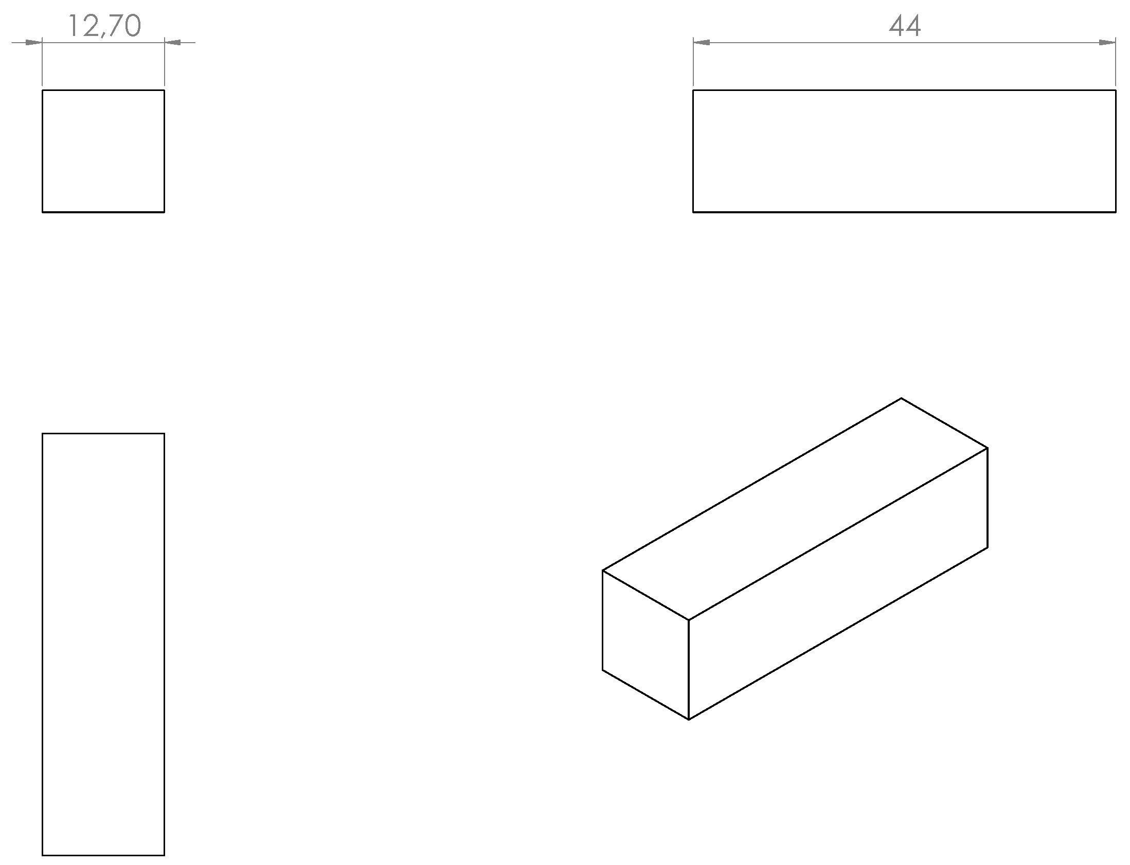
Figure 5.
Artisan QTest10 [27] testing machine during an experimental tensile test.
Figure 5.
Artisan QTest10 [27] testing machine during an experimental tensile test.
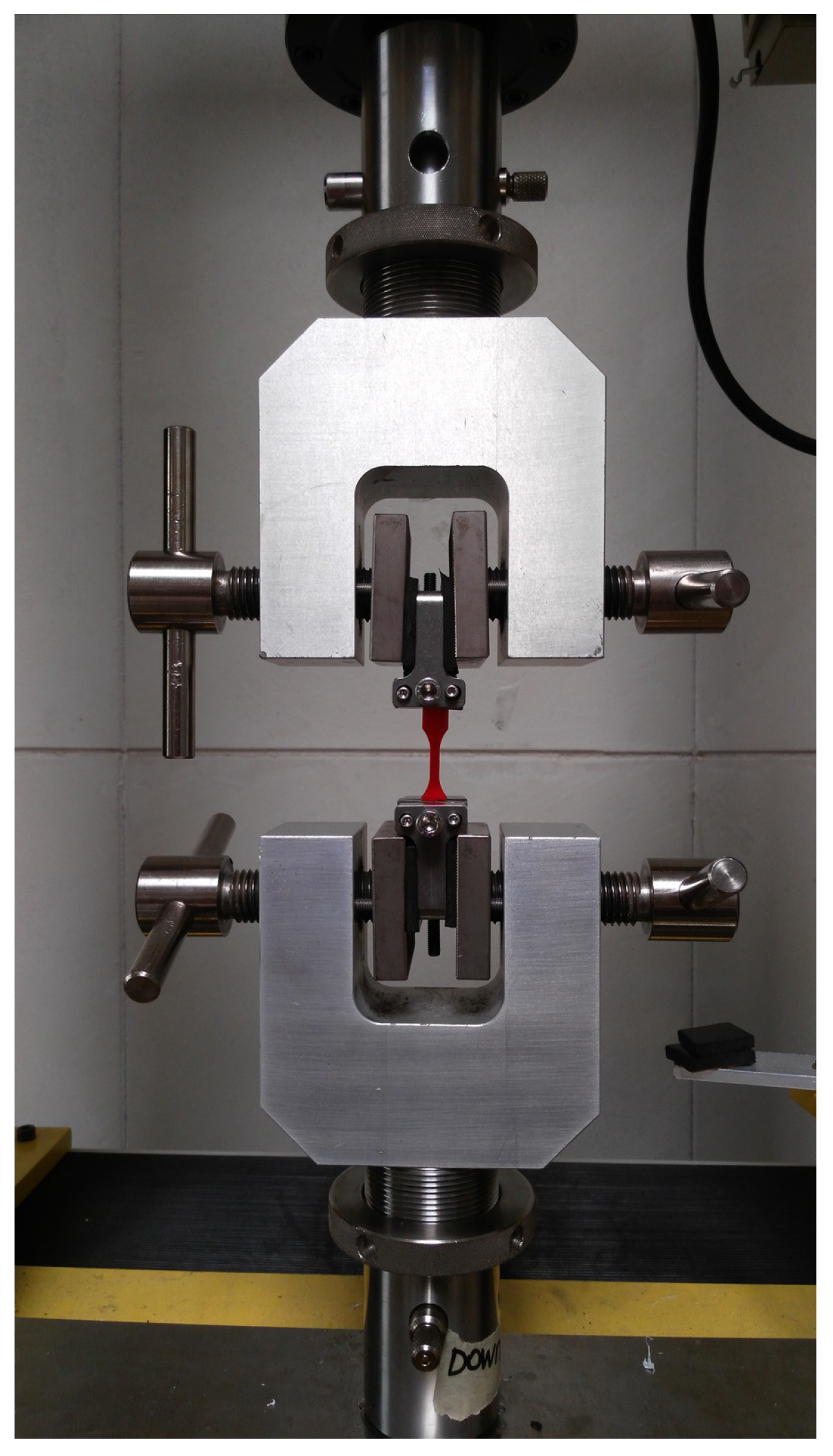
Figure 6.
Raw stress-strain curves for the nine produced specimens.

Figure 7.
The possible deformation modes in a compression test.

Figure 8.
The behavior of the fourth specimen during the compression test.
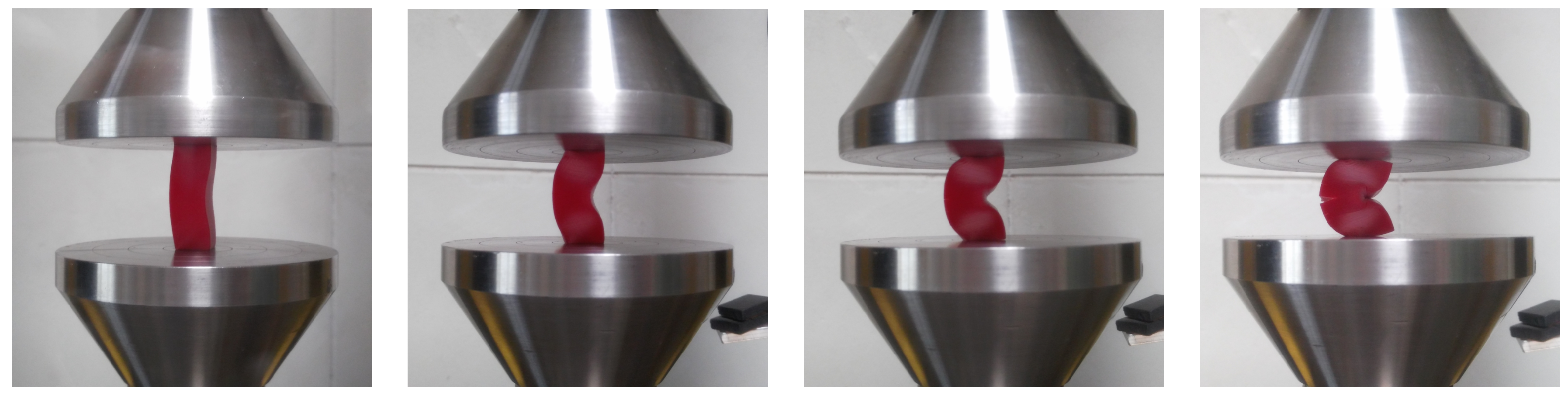
Figure 9.
Condition of the fourth specimen after the compression test.

Figure 10.
Actual stress-strain curve for the produced Specimen 2.

Figure 11.
Actual stress-strain curve for the produced Specimen 3.

Figure 12.
Actual stress-strain curve for the produced Specimen 4.
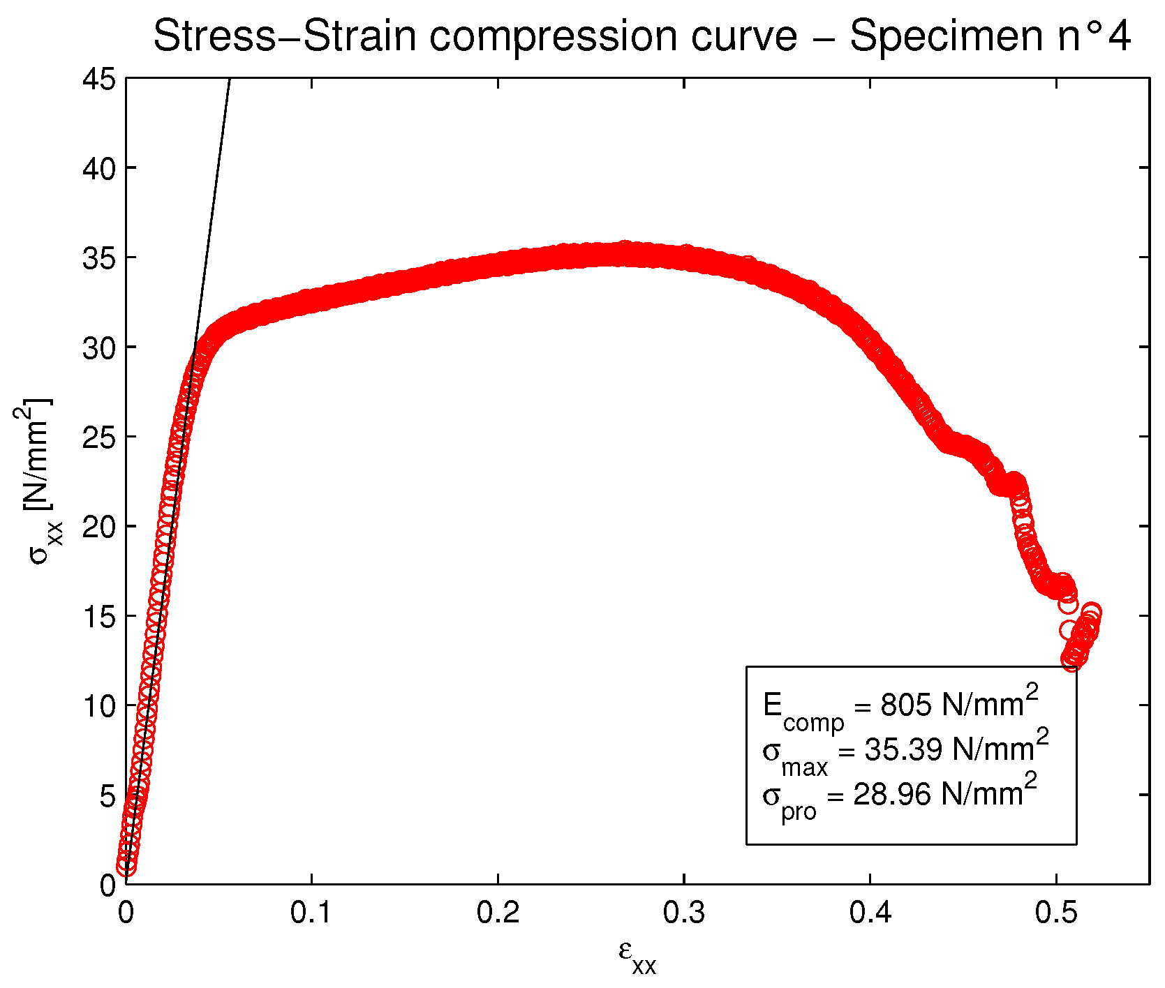
Figure 13.
Actual stress-strain curve for the produced Specimen 5.

Figure 14.
Actual stress-strain curve for the produced Specimen 6.

Figure 15.
Actual stress-strain curve for the produced Specimen 7.

Figure 16.
Actual stress-strain curve for the produced Specimen 8.

Figure 17.
Actual stress-strain curve for the produced Specimen 9.
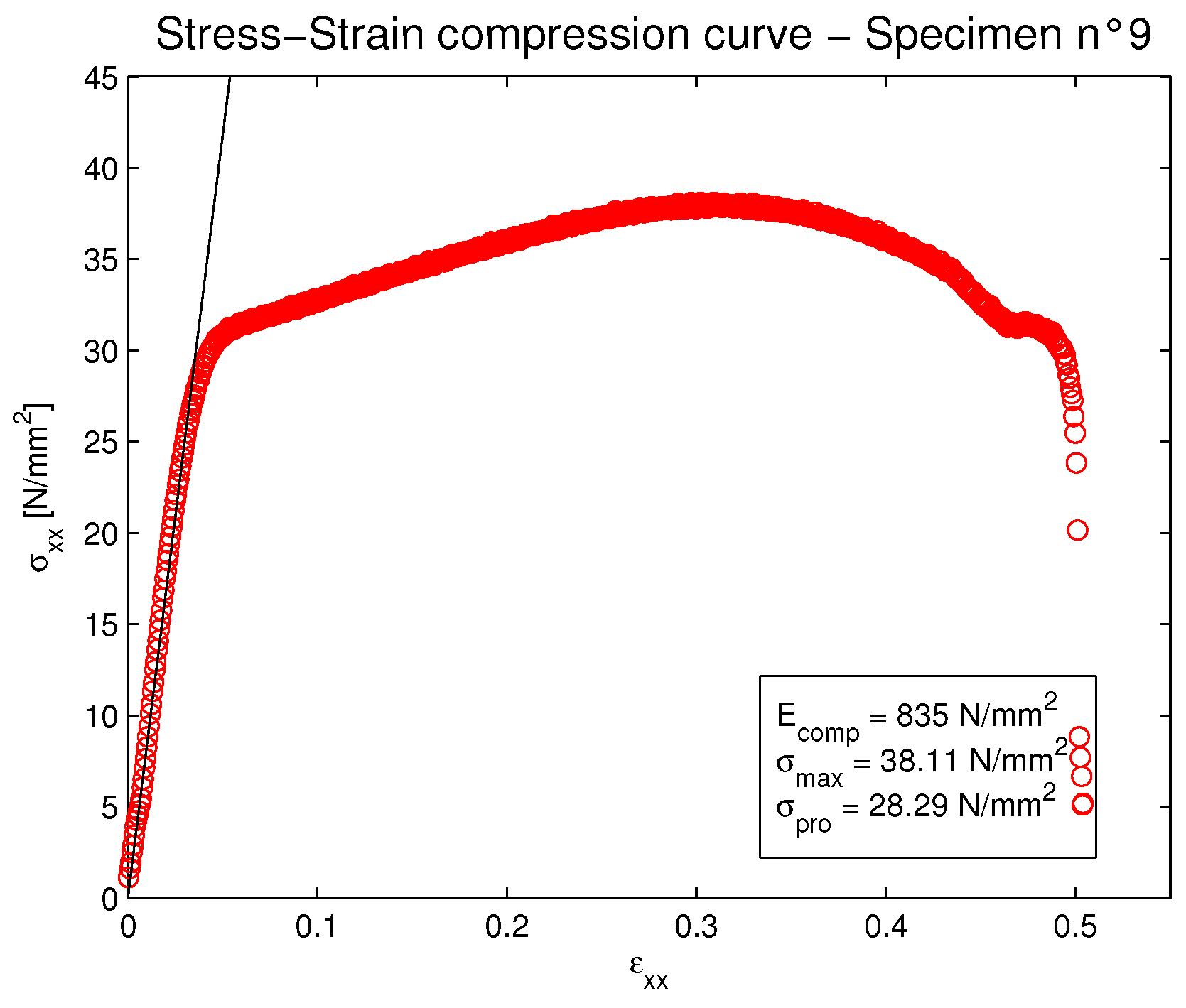
Figure 18.
Actual stress-strain curve for the produced Specimen 10.
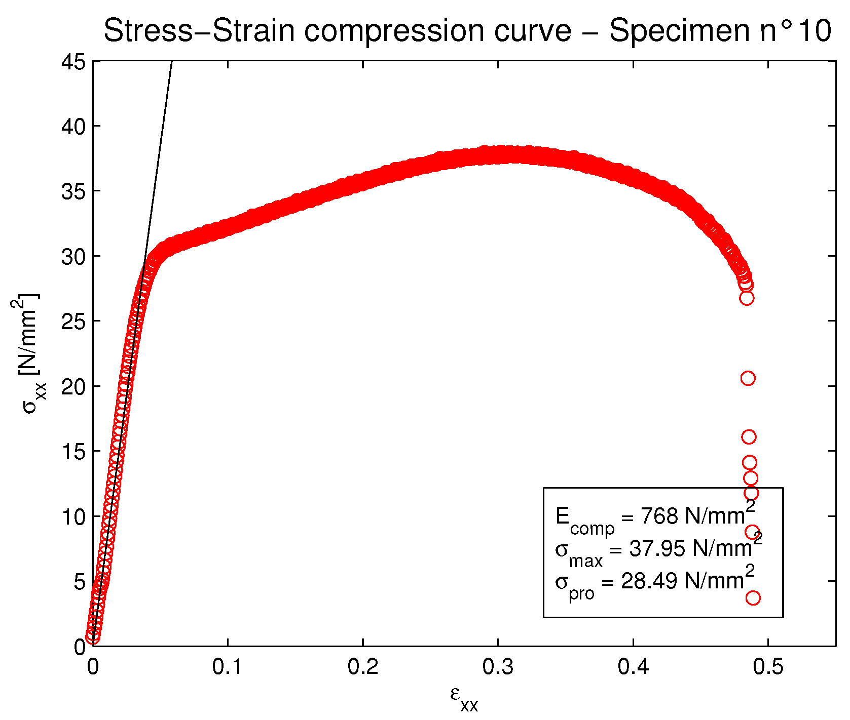
Figure 19.
Probability plot, process capability report and I-MR chart (Individuals (I) chart and Moving Range (MR) chart) for the Young modulus E of the nine produced specimens.
Figure 19.
Probability plot, process capability report and I-MR chart (Individuals (I) chart and Moving Range (MR) chart) for the Young modulus E of the nine produced specimens.

Figure 20.
Probability plot, process capability report and I-MR chart (Individuals (I) chart and Moving Range (MR) chart) for the maximum stress at rupture () of the nine produced specimens.
Figure 20.
Probability plot, process capability report and I-MR chart (Individuals (I) chart and Moving Range (MR) chart) for the maximum stress at rupture () of the nine produced specimens.

Figure 21.
Probability plot, process capability report and I-MR chart (Individuals (I) chart and Moving Range (MR) chart) for the stress at proportional limit () of the nine produced specimens.
Figure 21.
Probability plot, process capability report and I-MR chart (Individuals (I) chart and Moving Range (MR) chart) for the stress at proportional limit () of the nine produced specimens.

Figure 22.
Probability plot, process capability report and I-MR chart (Individuals (I) chart and Moving Range (MR) chart) for the X dimension of the nine produced specimens.
Figure 22.
Probability plot, process capability report and I-MR chart (Individuals (I) chart and Moving Range (MR) chart) for the X dimension of the nine produced specimens.

Figure 23.
Probability plot, process capability report and I-MR chart (Individuals (I) chart and Moving Range (MR) chart) for the Y dimension of the nine produced specimens.
Figure 23.
Probability plot, process capability report and I-MR chart (Individuals (I) chart and Moving Range (MR) chart) for the Y dimension of the nine produced specimens.

Figure 24.
Probability plot, process capability report and I-MR chart (Individuals (I) chart and Moving Range (MR) chart) for the length of the nine produced specimens.
Figure 24.
Probability plot, process capability report and I-MR chart (Individuals (I) chart and Moving Range (MR) chart) for the length of the nine produced specimens.

Figure 25.
Probability plot, process capability report and I-MR chart (Individuals (I) chart and Moving Range (MR) chart) for the weight of the nine produced specimens.
Figure 25.
Probability plot, process capability report and I-MR chart (Individuals (I) chart and Moving Range (MR) chart) for the weight of the nine produced specimens.


Table 1.
Dimensional experimental data for the nine produced ABS specimens.
| Specimen | ||||||||||||
|---|---|---|---|---|---|---|---|---|---|---|---|---|
| X dimension (mm) | ||||||||||||
| Y dimension (mm) | ||||||||||||
| Length (mm) | ||||||||||||
| Weight (g) |
Note: Nominal values (Nominal), mean values (Mean) and Standard Deviation (StDev).
Table 2.
Mechanical experimental data for the compression test of the 9 produced specimens.
| Specimen | |||||||||||
|---|---|---|---|---|---|---|---|---|---|---|---|
| E (MPa) | 881 | 879 | 805 | 711 | 825 | 721 | 821 | 835 | 768 | ||
| (MPa) | |||||||||||
| (MPa) |
Note: Mean values (Mean) and Standard Deviation (StDev).
Table 3.
Individual distribution identification for the compression modulus of elasticity, the compressive stress at rupture and the compressive proportional limit .
Table 3.
Individual distribution identification for the compression modulus of elasticity, the compressive stress at rupture and the compressive proportional limit .
| Goodness of Fit Test | Compression Modulus | |||||
|---|---|---|---|---|---|---|
| Normal | ||||||
| Box–Cox transformation | ||||||
| Lognormal | ||||||
| 3-Parameter lognormal | − | − | − | |||
| 2-Parameter Exponential | >0.250 | |||||
| Weibull | >0.250 | >0.250 | >0.250 | |||
| N3-parameter Weibull | >0.500 | >0.500 | ||||
| Smallest extreme value | >0.250 | >0.250 | ||||
| Largest extreme value | >0.250 | |||||
| Gamma | >0.250 | >0.250 | ||||
| Logistic | >0.250 | >0.250 | >0.250 | |||
| Loglogistic | >0.250 | >0.250 | ||||
| 3-Parameter Loglogistic | − | − | − | |||
Table 4.
Individual distribution identification for the width, the thickness, the length and the weight of the produced specimens.
Table 4.
Individual distribution identification for the width, the thickness, the length and the weight of the produced specimens.
| Goodness of Fit Test | Width: X Dimension | Thickness: Y Dimension | Length | Weight | ||||
|---|---|---|---|---|---|---|---|---|
| Normal | ||||||||
| Box–Cox transformation | ||||||||
| Lognormal | ||||||||
| 3-Parameter lognormal | − | − | − | − | ||||
| Exponential | − | − | − | − | <0.003 | <0.003 | ||
| 2-Parameter exponential | >0.250 | |||||||
| Weibull | >0.250 | >0.250 | ||||||
| 3-Parameter Weibull | >0.500 | >0.500 | ||||||
| Smallest extreme value | >0.250 | >0.250 | ||||||
| Largest extreme value | >0.250 | >0.250 | ||||||
| Gamma | >0.250 | >0.250 | ||||||
| 3-Parameter gamma | − | − | − | − | − | − | ||
| Logistic | >0.250 | >0.250 | ||||||
| Loglogistic | >0.250 | >0.250 | ||||||
| 3-Parameter loglogistic | − | − | − | − | ||||
© 2017 by the authors. Licensee MDPI, Basel, Switzerland. This article is an open access article distributed under the terms and conditions of the Creative Commons Attribution (CC BY) license (http://creativecommons.org/licenses/by/4.0/).
Share and Cite
MDPI and ACS Style
Brischetto, S.; Ferro, C.G.; Maggiore, P.; Torre, R. Compression Tests of ABS Specimens for UAV Components Produced via the FDM Technique. Technologies 2017, 5, 20. https://doi.org/10.3390/technologies5020020
AMA Style
Brischetto S, Ferro CG, Maggiore P, Torre R. Compression Tests of ABS Specimens for UAV Components Produced via the FDM Technique. Technologies. 2017; 5(2):20. https://doi.org/10.3390/technologies5020020
Chicago/Turabian StyleBrischetto, Salvatore, Carlo Giovanni Ferro, Paolo Maggiore, and Roberto Torre. 2017. "Compression Tests of ABS Specimens for UAV Components Produced via the FDM Technique" Technologies 5, no. 2: 20. https://doi.org/10.3390/technologies5020020
Note that from the first issue of 2016, this journal uses article numbers instead of page numbers. See further details here.