Multi-Factor Asset-Pricing Models under Markov Regime Switches: Evidence from the Chinese Stock Market


1
Graduate School of Commerce, Waseda University, Tokyo 169-8050, Japan
2
Graduate School of Business and Finance, Waseda University, Tokyo 169-8050, Japan
*
Author to whom correspondence should be addressed.
Int. J. Financial Stud. 2018, 6(2), 54; https://doi.org/10.3390/ijfs6020054
Submission received: 21 February 2018
/
Revised: 15 May 2018
/
Accepted: 16 May 2018
/
Published: 20 May 2018
(This article belongs to the Special Issue Asset Pricing and Portfolio Choice)
Abstract
:This paper proposes a Markov regime-switching asset-pricing model and investigates the asymmetric risk-return relationship under different regimes for the Chinese stock market. It was found that the Chinese stock market has two significant regimes: a persistent bear market and a bull market. In regime 1, the risk premiums on common risk factors were relatively higher and consistent with the hypothesis that investors require more compensation for taking the same amount of risks in a bear regime when there is a higher risk-aversion level. Moreover, return dispersions among the Fama–French 25 portfolios were captured by the beta patterns from our proposed Markov regime-switching Fama–French three-factor model, implying that a positive risk-return relationship holds in regime 1. On the contrary, in regime 2, when lower risk premiums could be observed, portfolios with a big size or low book-to-market ratio undertook higher risk loadings, implying that the stocks that used to be known as “good” stocks were much riskier in a bull market. Thus, a risk-return relationship followed other patterns in this period.
JEL Classification:
G10; G12; C32; G151. Introduction
The Modern Portfolio Theory (MPT), first introduced by Markowitz (1952), describes the relationship between risk and expected return statistically using mean-variance optimization. Modern finance theory, therefore, stepped onto a new stage. Based on the framework of MPT, the Capital Asset Pricing Model (CAPM) was proposed to promote the study of asset-pricing and was developed by Treynor (1961, 1962), Sharpe (1964), Lintner (1965a, 1965b), and Mossin (1966). However, as more and more abnormal cross-sectional returns were found to be persistent and were unable to be explained by traditional asset-pricing models, Fama and French (1992, 1993) proposed a three-factor model in which the risk factors, such as MKT(Market), SMB (Small Minus Big), HML (High Minus Low), had an explanatory power on abnormal returns. Many researchers try to use multi-factor models to interpret anomalies in areas such as momentum and investment. By constructing several characteristic-based factors, such as the momentum-based factor UMD (Up Minus Down, Carhart 1997), the profitability-based factor RMW (Robust Minus Weak, Fama and French 2015, 2016), and the investment-based factor AGR (Asset Growth Return, Chen 2017), the multi-factor asset-pricing models are improved and can explain most of the characteristics related to abnormal returns.
Although the mean-variance model, CAPM, and the multi-factor model are logically simple and useful in practice, they are static, single-period linear models, which can hardly fit the real world risk-return relationship in the long run (Rossi and Timmermann 2010; Cotter and Salvador 2014). Using dynamic programming and stochastic analysis, Merton (1969, 1971) takes the investment opportunity set into consideration and expands the CAPM from single-period to multi-period, establishing the dynamic portfolio theory, known as the Intertemporal Capital Asset Pricing Model (ICAPM). Nevertheless, as Merton (1973) predicted in his ICAPM, the investment opportunities may vary with time, suggesting a conditional risk-return relationship. However, as He et al. (1996), Ferson and Harvey (1999), and Ghysels (1998) have pointed out, a lot of conditional asset-pricing models fail in their empirical performance and hardly capture the beta risk dynamics. We address this problem by putting multi-factor asset-pricing models under the Markov regime switching (MRS) framework, in which regime switches follow a Markov chain rule, and observations will be continuous in the time horizon. Since an MRS model can catch structure changes in economic dynamics, market structure, or other unexpected shocks in the time-series, an MRS adjusted multi-factor model combines the superiorities of linear and non-linear models.
Many studies have attempted this method. Coggi and Manescu (2004) presented a state-dependent version of the Fama–French three-factor model (1993). They found two separate regimes coexisting in the US market, one of which had higher factor loadings regarding the HML factor. Guidoline and Timmermann (2007, 2008) showed that size effect and book-to-market ratio (B/M) effect are strong in a bull state and diminished around a bear regime. Ozoguz (2008) also used a two-state regime-switching model and found a negative relationship between the level of uncertainty and asset valuations. The conditional model is successful in explaining part of the cross-sectional variation in average portfolio returns. Ammann and Verhofen (2009) adopted a Markov Chain Monte Carlo method to modify the Carhart (1997) four-factor model. They found that in a high-variance regime, only value stocks perform well, while in low-variance regimes, market portfolio and momentum stocks have higher returns. Abdymomunov and Morley (2011) investigated the time-variations in CAPM betas for B/M and momentum sorted portfolios under different market volatility regimes, and found that regime switching conditional CAPM can better explain stock returns than an unconditional CAPM. Mulvey and Zhao (2011) explored a non-linear factor model for allocating assets over the short run. Cotter and Salvador (2014) also developed a regime switching multi-factor framework to explore the risk-return relationship. They found that a positive and significant risk-return relationship occurred during periods of low volatility, while a relationship could not be observed during periods of high volatility.
Though past studies have tried to combine the multi-factor model with a regime switching framework, none of them have systematically investigated the time-variations in both, risk factors excess returns and risk loadings (known as betas). It is also vital to make comparisons among major asset-pricing models. Last, but not least, few researchers have investigated the time-varying risk-return relationship in the Chinese stock market. As the Chinese economy has had tremendous growth during the last 30 years, it has become one of the biggest markets in the world. Along with its economic growth, the Chinese financial market is also growing fast and has played an important role in the Asian-Pacific area. However, unlike other important stock markets, the Chinese stock market still faces serious problems that have been caused by the dual economic system, restrictions on foreign currency conversion, government interventions, and information asymmetries. Since the Chinese stock market is immature, highly restricted, and less inclusive, it is driven more by liquidity and speculative sentiment, rather than by economic fundamentals. That is why China has spent more than half of its time in a bear market, which has also been confirmed by our results. On the other hand, a bull state occurs from time to time, along with interventions by the government. Every time the government tries to “stabilize” a market or issue new policies, it brings a short period of prosperity dominated by irrational retail investors and speculators. As Brunnermeier et al. (2017) show in their theoretical model, although government intervention helps stabilize such an unregulated market, it also amplifies the effects of policy errors and worsens informational efficiency. Based on their predictions, we expect that the validity of equilibrium models may be distorted during some periods when pricing errors are increased by noise factors. Moreover, since Lin et al. (2012) and Guo et al. (2017) point that Fama-French factors can proxy the latent risk factors in the Chinese stock market, we focus on the two typical asset-pricing models (i.e., CAPM and Fama–French three-factor model) and put them under Markov regime switches. It was found that the Chinese stock market can be depicted with two regimes in which the multi-factor asset-pricing model deviates from one to the other. Hence, investigations on the features of the Chinese stock market, and the portraits of time-varying risk factors and betas, are of great significance to investors.
In this paper, we study two typical multi-factor asset-pricing models under the Markov regime switches for the Chinese stock market. We first distinguish different market states and examine the time-varying risk factors. Then, we allow risk loadings (i.e., betas) to switch across regimes. The results may shed light on the state-dependent risk-return relationship.
2. Data and Methodology
2.1. Data
2.1.1. Benchmark Portfolios
Following the conventions of Fama and French (1996, 2006), we constructed 25 portfolios (denoted as FF25) based on quintile intersections of size and B/M, and take them as the benchmark portfolios. We studied all firms that were listed on the Shanghai Stock Exchange and the Shenzhen Stock Exchange, during the period from July 1995 to March 2015. However, since stock returns from July of year t to June of year t + 1 are matched with the accounting data in December of year t – 1, firms that did not have December fiscal year-end data or 36 months of stock return data were excluded from the dataset. Every year, at the end of June, all stocks were ranked and allocated by their size quintile cutoffs and B/M quintile cutoffs. The size breakpoints of year t were the market capitalizations of each stock by the end of June of year t. The B/M for June of year t is the book value of year-end t – 1 divided by the market value in December of year t – 1. Then, the 25 portfolios were held for a year and the monthly average raw returns for each portfolio were calculated.
2.1.2. Constructing Risk Factors
Based on the methodology of Fama and French (1993), at the end of June every year, all the sample stocks were divided into six groups based on their size and B/M value cutoffs. The size breakpoint was the median market capitalization of all stocks at the end of June of year t. The B/M breakpoint for June of year t was the book value of last fiscal year-end in December year t – 1 divided by market equity for December year t – 1. Based on the cutoffs, growth portfolio was composed of the lowest 30% B/M firms, while value group included the highest 30% B/M firms. The remaining 40% of stocks comprised the medium group. Following Equations (1) and (2), value-weighted return difference between the value and growth portfolios within each of the size groups was calculated and averaged. The return difference was a value common risk factor, denoted by HML. We adopted the same approach to calculate SMB. Table 1 presents the formation of the common risk factor. The market risk factor was also the excess return on the market portfolio.
HML = (RS/H + RB/H − RS/L − RB/L) ÷ 2
SMB = (RS/L + RS/M + RS/H − RB/L − RB/M − RB/H) ÷ 3
2.2. Methodology and Models
2.2.1. The Framework of a Markov Regime-Switching Model
The MRS is a flexible framework that is proficient in handling the variations caused by heterogeneous states of the world. In this paper, we focused on the regime-dependent risk factors and risk loadings in multi-factor models. Following the conventions of Hamilton (1989, 1994), we modeled the regimes as follows.
For a regime-switching model, the transition of states is stochastic. However, the switching process followed a Markov chain and was driven by a transition matrix, which controls the probabilities of making a switch from one state to another. Considering that the Chinese stock market has manifested bear and bull markets, which along with business cycles, vary between expansions and recessions, we allowed two states, namely, a bear state and a bull state, in this model. The transition matrix is represented as:
where Pij is the probability of switching from state i to state j.
Denoting as the matrix of available information at time t – 1, the probability of State 1 or 2 is calculated following Equations (4) and (5):
To estimate a regime-switching model where the states are unknown, we consider as the likelihood function for state j on a set of parameters (Θ). Then the full log likelihood function of the model is given by:
which is a weighted average of the likelihood function in each state, and the weights are the states’ probabilities. Applying Hamilton’s filter, the estimates of probabilities can be acquired by doing an iterative algorithm. Finally, the estimates in the model were obtained by finding the set of parameters that maximized the log likelihood equation.
To investigate a time-varying risk-return relationship, we put the multi-factor asset-pricing models under Markov regime switches. We first analyzed time-series variations in risk premiums for each risk factor by using a multivariate MRS model. Then we allowed beta in the multi-factor asset-pricing model to switch under a univariate MRS setting. Two models were adopted in this research. The first model was the CAPM, including the market factor (MKT). The second model was the Fama–French three-factor model, which incorporates the size factor (SMB) and value factor (HML).
2.2.2. CAPM with Markov Switching (MR–CAPM)
In the case of a CAPM, the market risk factor was first studied to identify two regimes.
with:
where is the market risk premium, St is an indicator variable that denotes the possible two states, is the residual vector that follows the normal distribution, and is the variance vector at state St.
In the second step, the market beta and residual in CAPM were assumed to be regime-dependent.
where is the excess return for portfolio i, is the unexplained return, is the risk loading, and is excess return on market portfolio. St is an indicator variable that denotes the possible two states. is the residual vector that follows the normal distribution and is the variance vector at state St.
The model was applied independently for the 25 benchmark portfolios. The matrix of estimates for parameters in the model is reported in section three.
2.2.3. Fama–French Three-Factor Model with Markov Switching (MR-FF3 Model)
In a Fama–French three-factor model, three factors (i.e., the market factor (MKT), the size factor (SMB), and the value factor (HML)) are proposed to explain the size anomaly and value anomaly. According to the formation of common risk factors, SMB and HML are history returns on the hedging portfolios (small minus big, high B/M minus low B/M), known as RSMB and RHML. So, if these factors (i.e., SMB and HML) originate from the portfolios/stocks in the market, and the return series emerge from the market, it is sagacious to guess that SMB and HML factors in the Fama–French three-factor model may vary over time and could be non-linear dynamic.
Therefore, the risk premiums for the common risk factors can be represented as a matrix λ:
Since the common risk factors are mimicking portfolios, excess returns on risk factors have no autoregressive terms, following a simple mean-variance MRS model:
with:
where St is an indicator variable that denotes the possible two states. , , and refer to the residual vectors for MKT, SMB, and HML, and follow the normal distribution. , , and are the variance vectors for the three factors at state St.
In the second step, betas for three factors and the residual in the Fama–French three-factor model are assumed to be regime-dependent.
where is the excess return for portfolio i, is the unexplained return, , , are the risk loadings on three factors, and , , are the three factors. St is an indicator variable that denotes the possible two states. is the residual vector that follows the normal distribution. is the variance vector at state St.
Similarly, the MR-FF3 model will be estimated for each of the 25 portfolios.
3. Empirical Results
In this section, we present the estimates of multi-factor asset-pricing models under Markov regime switches. First, in the market process, we conducted the multivariate MRS model to analyze the regime-dependent variations among common risk factors. Then, in the beta process, a univariate MRS model is applied to investigate variations in risk loadings.
3.1. Estimation of MR-CAPM
3.1.1. Risk Factor Variations
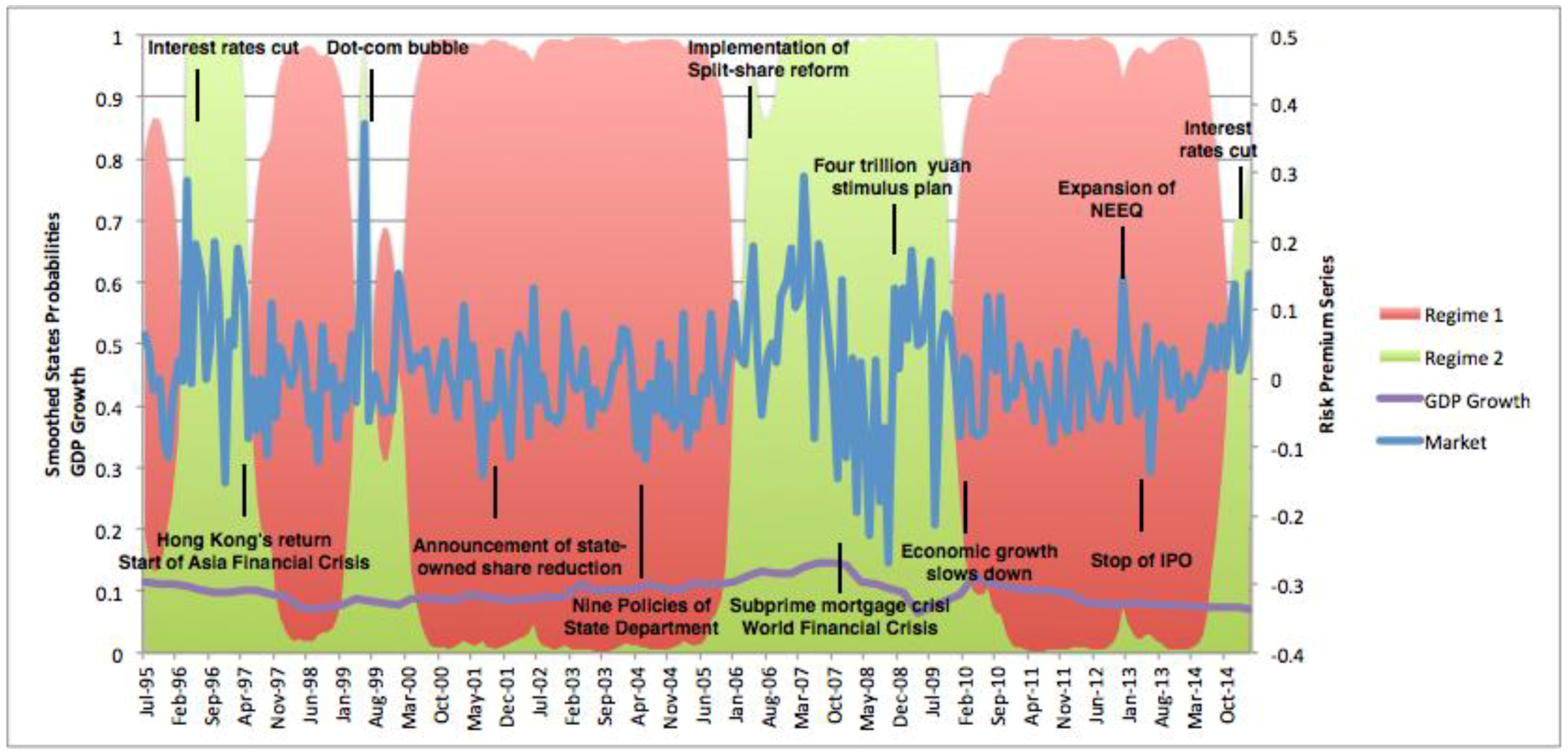
In the market process, we first analyzed the risk factor variations under Markov switching to determine regimes. Following the model developed in Section 2.2.2, we applied the Perlin (2014) Matlab Package and estimated the parameters, as shown in Table 2 and Figure 1, determining the two regimes as a bear and a bull state, respectively.
Figure 1 plots the conditional mean of market return and the smoothed probablilities of regimes 1 and 2 in the sample period. The red area refers to the smoothed probability of regime 1, while the green area implies that of regime 2. At any time point, the sum of probablilities of regimes 1 and 2 should be equal to one. It is shown that regime 1 dominated most of the sample period, inferring that the Chinese stock market has been a bear market for most of the time. Further, if we compare the period of regime 2 with real world events that occurred in the time horizon, we can find that regime 2 has captured most of the astonishing booms and crises, and ups and downs. The market was inspired before Hong Kong returned to China in 1997. However, as the Asian financial crisis hit the Hong Kong market, the Chinese stock market also came to a bear state. In 2000, the international dot-com bubble occured, and the Chinese stock market experienced a short rise before coming to a long bear state from 2001 to 2006, because the state-owned shares (previously illiquid shares) were reduced and dumped into the market. Then, in 2006, as the government released several policies related to the split-share reform, the market stepped into a bull regime. However, speculations were driven by irrationalities, as it was more or less like a bubble. Along with the snow disaster in southern China and the Wenchuan earthquake, following the overwhelming subprime crisis along with the global economic slowdown, the Chinese stock market was dragged into another bear regime.
Table 2 shows that the conditional mean of market return is relatively lower in regime 1, but higher in regime 2, aligning with the definitions of regimes 1 and 2. The transition matrix reveals that the probability of switching from bear to bull is 0.03, which is smaller than the probability of switching from bull to bear (0.06). If the current state is regime 1, it is less likely to switch to the bull market, because the probability of keeping the current state is 0.97. Hence, it is natural to find that the expected duration of staying at a bear market is 34.05 months, which is much longer than that of a bull market. Thus, the Chinese market has remained a bear market for most of the time.
3.1.2. Risk Loading Variations
In the beta process, we allow risk loading for each risk factor to switch across regimes. Figure 2 plots the market betas in the MR-CAPM model for the 25 characterized portfolios.
The left subfigure plots the estimates in regime 1, and the right subfigure plots the estimates in regime 2. In both regimes, the market betas are non-zeros. If we compare two typical characterized portfolios, P5 (the 5th portfolio characterized by the highest B/M and the smallest size) and P21 (the 21st portfolio characterized by the lowest B/M and the biggest size), it will help reveal the return dispersions among portfolios. The risk loading of P5 is higher than the loading of P21 in regime 1, but the relation is reversed in regime 2. Thus, we can say that the return dispersion between P5 and P21 is explained by the risk dispersion between P5 and P21 in regime 1. However, the risk explanation no longer holds in regime 2. Thus, in a bear market, a positive risk-return relationship holds, while in a bull market, the trade-off between risk and return follows other patterns.
3.2. Estimation of MR-FF3 Model
3.2.1. Risk Factor Variations
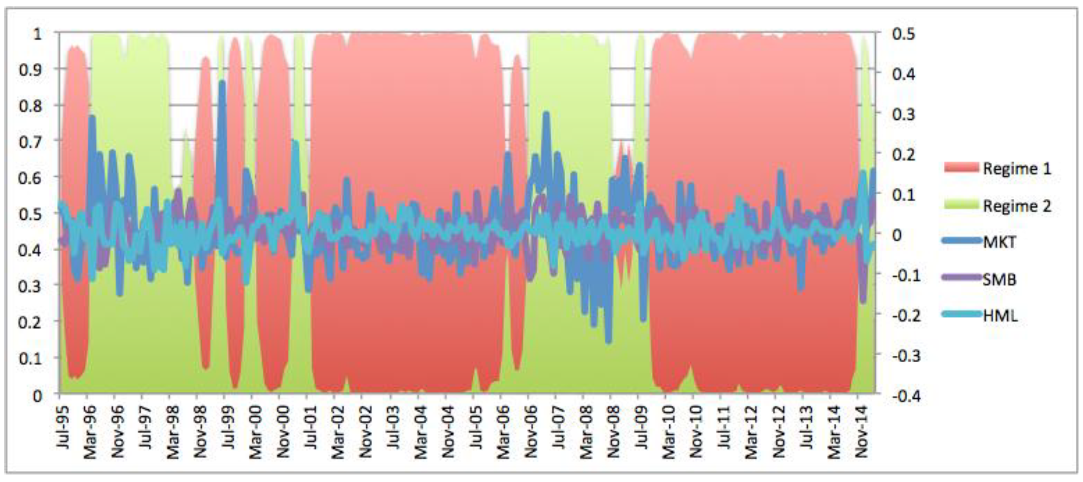
To better understand how the risk-return relationship deviates, we put the traditional Fama–French three-factor model in the framework of Markov regime switches. We first analyzed how risk factors vary as regime switches. Figure 3 plots the time-series variations of risk premiums on MKT, SMB, and HML. The red and green areas denote the smoothed probabilities of a bear market (regime 1) and a bull market (regime 2), respectively. It was shown that a bear market dominated most of the observation period. According to the estimates in Table 3, if the current state is a bear market, the probability of staying at the current state is as high as 0.95. Further, since the probability of transmitting from bear to bull is 5%, lower than the probability of transmitting from bull to bear (11%), it is more likely to be a bear market, whose expected duration is as long as 18.89, almost twice that of a bull market.
Table 3 provides the estimates of parameters in the MR-FF3 model. Aligning with the findings in Chen (2017), in a bear market (regime 1), the risk premiums of SMB and HML was slightly higher. It is because in a bear market, when the market return is low and the business is under downturn, investors ask for higher compensation on size-related risk and value-related risk. According to Cochrane (2005), during bad times, when investors value a little bit of extra wealth, “good” stocks that pay off well are wanted by investors and get a higher price. Other stocks that cannot provide good payoffs in these times are “bad” stocks and will have a lower price with a higher expected return. Then, the return dispersions between “bad” and “good” stocks are expected to expand. Therefore, return dispersions between “small” and “big” stocks and “high B/M” and “low B/M” stocks are expected to expand, and thus, risk premiums on SMB and HML are higher in a bear market.
However, in a bull market, when the market return is high, investors ask for lesser compensation. This is consistent with the expectation that during the bull market, risk-loving investors that ask for a lower price of risk for a unit of risk are increasing. Thus, in regime 1, as the risk premiums in SMB and HML are higher, the risk-aversion levels in the market are also increasing. However, in regime 2, following the same rule, the risk-aversion levels in the market are decreasing.
3.2.2. Risk Loading Variations
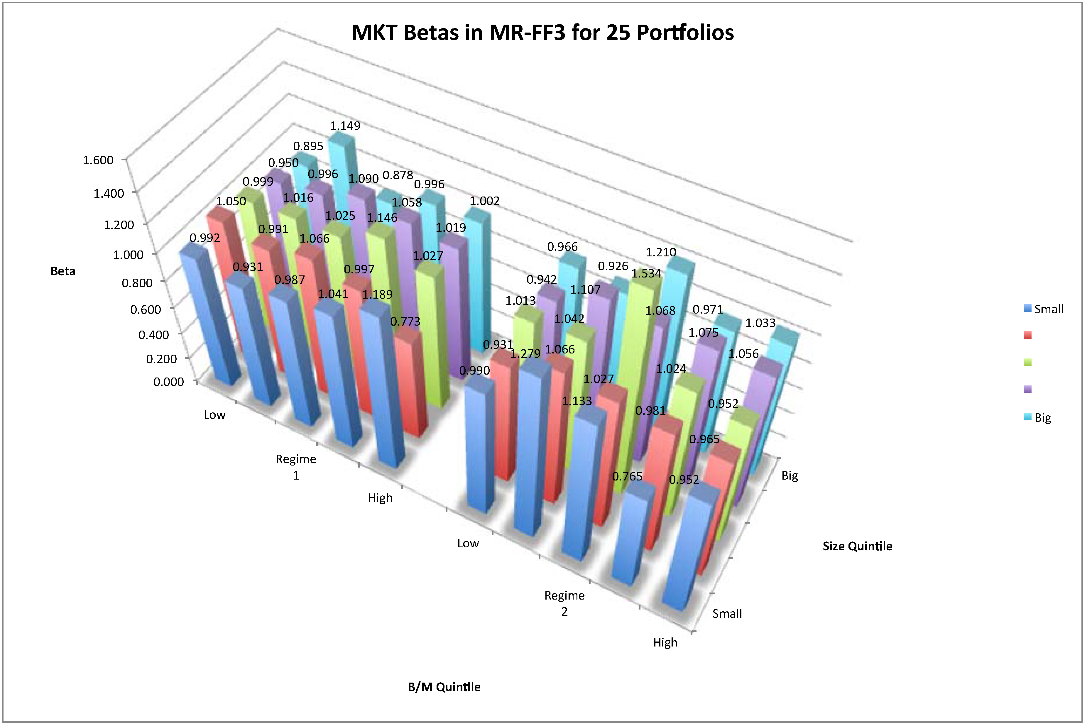
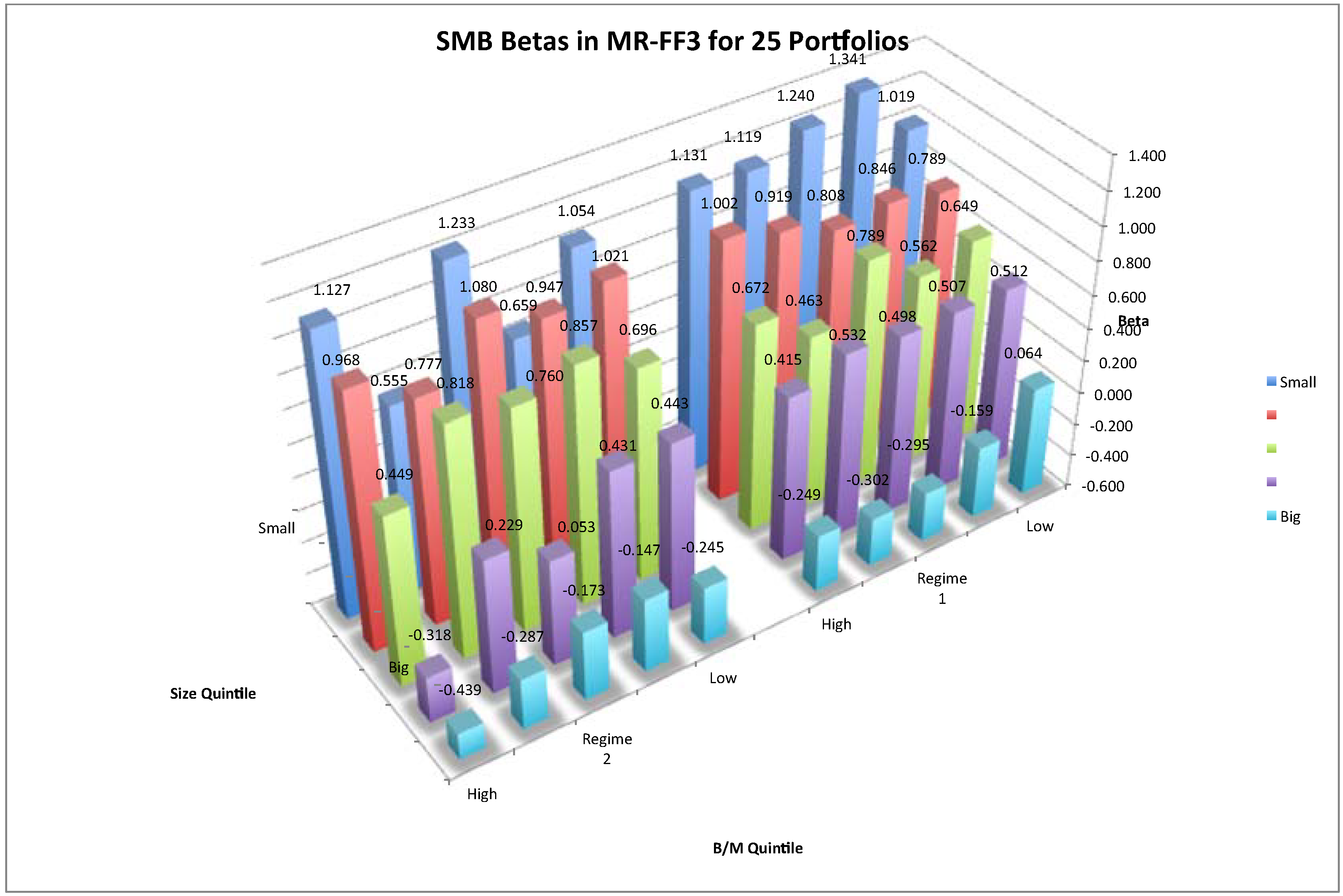
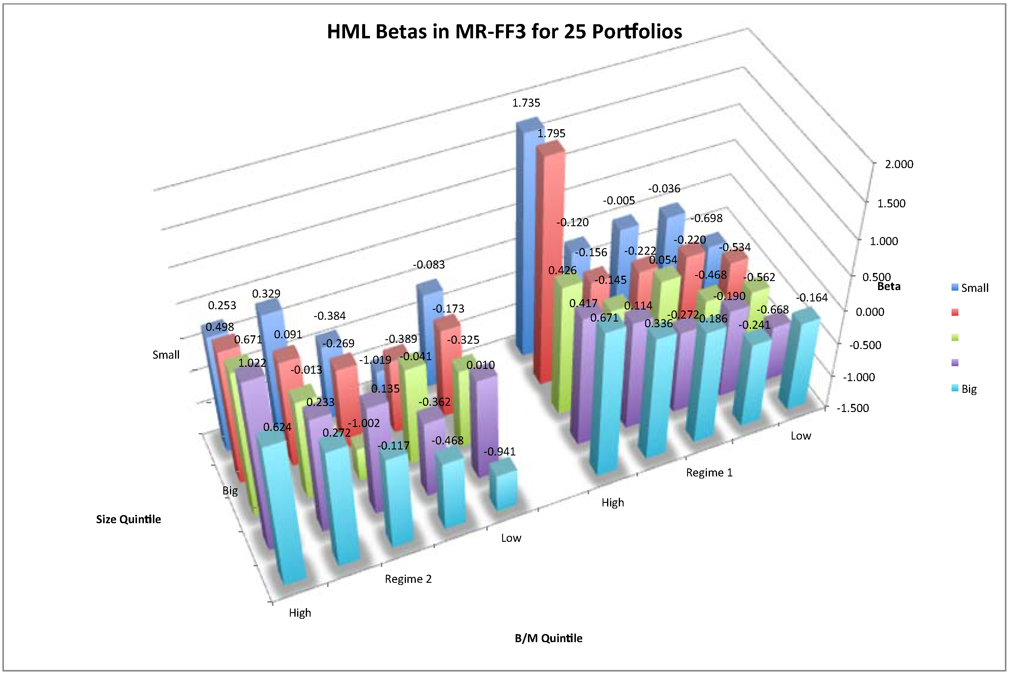
Adopting the same approach as in Section 3.1.2, we allow risk loadings of the MR-FF3 model to vary across regimes. Figure 4, Figure 5, Figure 6 plotings on MKT, SMB, and HML in the MR-FF3 model for the 25 characterized portfolios, respectively the risk load.
In either figure, the subfigures plot estimates for regime 1 and regime 2, respectively. It is shown that in regime 1, risk loadings on SMB and HML have typical patterns. In regime 1, betas of SMB factor increased as the size of each portfolio decreased from big to small. Thus, return dispersions between big and small stocks were captured by the SMB factor. Meanwhile, betas of HML factor increased as B/M value of each portfolio increased, implying that return dispersions between low and high B/M stocks were captured by HML factors. Therefore, it is in regime 1 that a three-factor asset-pricing model can explain the expected returns on stocks. However in regime 2, beta loadings had a reversed pattern, in that big size and low B/M portfolios had higher risk loadings. Thus, in a bull market, investing on such big and low B/M stocks may undertake higher risks, and a positive risk-return relationship no longer holds.
3.2.3. Robustness Test Using a Hedging Portfolio
To compare the performance of unconditional factor models and regime-dependent factor models, we further conducted a time-series regression of excess returns for a hedging portfolio on risk factors. The hedging portfolio is a zero-cost portfolio that has a long position on the 5th portfolio of FF25 portfolios, and a short position on the 21st portfolio of the FF25 portfolios, denoted as a “5–21” portfolio. Because the 5th portfolio was the one that had the smallest size and the highest B/M value, while the 21st portfolio was the one that had the biggest size and the lowest B/M value, return spreads between the two portfolios should be the largest and related with firm characteristics of size and B/M. Table 4 reports the estimates of exposures to risk factors for each of the four models: unconditional CAPM, MR-CAPM, unconditional FF3 model, and MR-FF3 model. As is shown in Panel A of Table 4, the unconditional CAPM fails to explain the abnormal return of the hedging portfolio because there is a significant intercept and an insignificant market beta. However, when the model is conditioned on regimes, we found that the CAPM had an asymmetric pattern under two regimes, in which regime 1 had a significant market beta. The Fama–French three-factor model was also improved by adjusting under Markov regime switches. The MR-FF3 model explained more unexplained returns and depicted a regime-dependent risk exposure pattern. Statistics in Panel B implied that am MR-FF3 model had the least pricing errors and best performance under different criterions.
3.3. Out-of-Sample Analysis on MR-FF3 Model
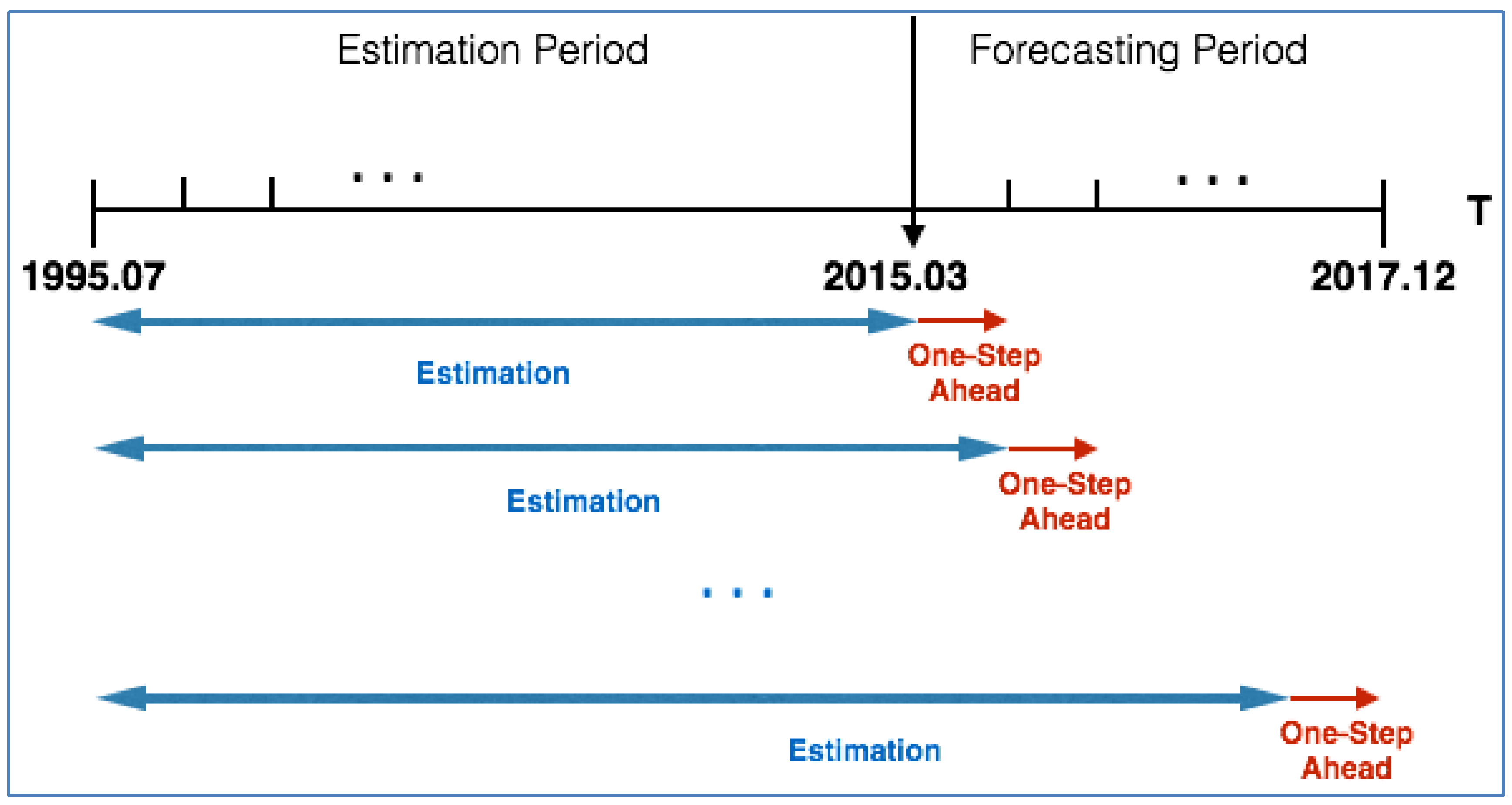
Based on the MR-FF3 model developed in Section 3.2, we conducted an out-of-sample analysis to examine its predictability. For each of the 25 portfolios, the estimation window ranged from July 1995 to March 2015, while the forecasting period ranged from April 2015 to December 2017. The MR-FF3 model was first estimated in the expanding window regressions, and then the Markov regime transition matrix and conditional mean parameters were estimated under a root mean squared prediction error (RMSPE) criterion.
is the one-step-ahead expected return under regime switching, which is a weighted average of the returns in Regime 1 and Regime 2, where the weights were given by the transition probabilities conditional on the prevailing state at time t, as shown in the following equation:
where is the mean forecast for each state:
Here in model MR-FF3:
where is the coefficient vector that depends on state (). is the realized factor return vector at t + 1, which is the independent data used to predict the expected return.
is calculated based on:
where is the transition probability matrix and is the filtered probability vector at t.
Therefore,
Based on the calculations above, we can estimate the one-step-ahead forecasts.
Since the estimation window incorporates all the previous information, it is an expanding window estimation. The forecasting horizon is one step, from t to t + 1, stepping over one month. Figure 7 illustrates the methodology adopted in this section.
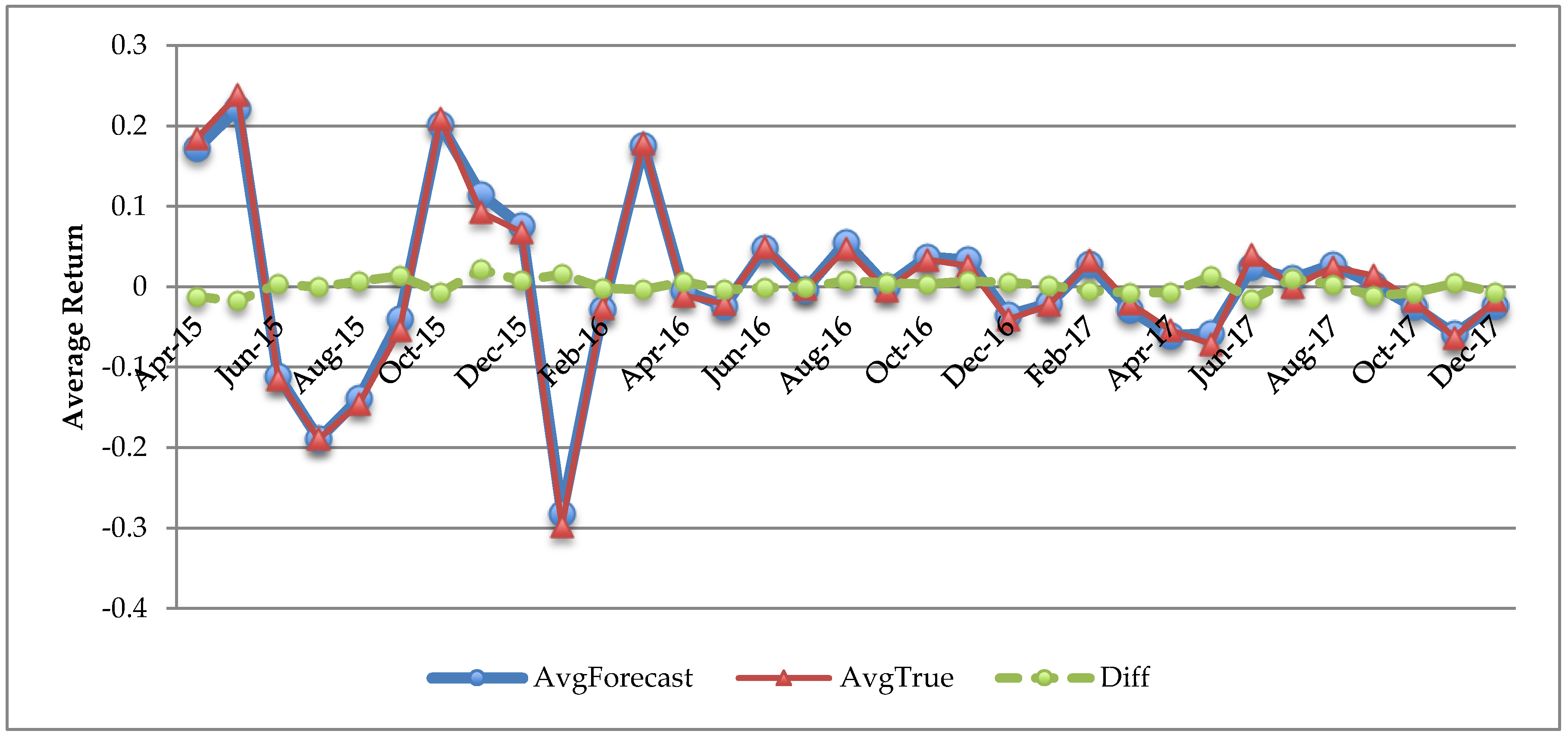
The out-of-sample analysis was conducted for each of the 25 Fama–French portfolios. Figure 8 plots the forecasting returns and actual returns for portfolios 1, 5, 21, and 25, respectively. Table 5 further reports the performance of the MR-FF3 model in in-sample and out-of-sample fitting. It was noticed that the in-sample RMSE was unusually larger than out-of-sample RMSE for the reason that idiosyncratic variance declined over time. Furthermore, we calculated the arithmetic average of the 25 portfolio estimated returns at each time point during the forecasting window. Figure 9 shows the average forecasting returns versus true values. It was shown that the differences between forecasting and true values were close to zero.
4. Discussion
In this study, we found that there were two significant regimes (i.e., bear and bull) existing in the Chinese stock market. It was shown that the bear market dominated most of the sample period, aligning with the fact that the Chinese stock market is still an emerging market and has been facing problems caused by dual economic characteristics and restrictions by government policies. On the other hand, the so-called bull market was characterized by increasing risk-takers (risk-lovers) in the market, generating lower risk premiums on common risk factors (i.e., SMB and HML).
To understand how asset-pricing models perform under different regimes, we first adjusted the CAPM by introducing the two regimes. It was found in regime 1 that a positive risk-return relationship was persistent when market beta was significantly positive. However, in a bull market, when there were negative betas, a trade-off between risk and return had other patterns.
Furthermore, we proposed a MR-FF3 model to investigate the risk-return trade-off deviations. We observed risk factor variations and risk loading variations across two regimes. It was found in regime 1 that the factor excess returns were relatively higher, consistent with the hypothesis that a bear market has a higher risk-aversion level. Moreover, investigations of the beta process implied that return dispersions among characterized portfolios came from risk loading patterns. Specifically, portfolios that have higher returns endure greater exposure to common risk factors (i.e., SMB and HML). Thus, a multi-factor asset-pricing model worked well in regime 1. However, in State 2, beta loadings had a reversed pattern, where portfolios characterized with a big size and low B/M had higher risk loadings. Meanwhile, since the risk price in regime 1 was higher than risk price in regime 2, the risk-return relationship did not hold any more in a bull market1. Moreover, we conducted an out-of-sample analysis on the Fama–French three-factor model under Markov regime switches. It was shown that an MR-FF3 model performed well in one-step-ahead forecasting.
To sum up, for an investor in the Chinese stock market, variations in risk factors dominated the changes from regime 1 to 2. Though investors do not know the exact current state, they could infer the market state based on information available from newspapers and government policies, especially from the estimates of excess returns on common risk factors. If it is in regime 1, investment strategies based on a three-factor model may be helpful. However, if it is in a bull market, when the multi-factor asset-pricing models deviate, investing on big stocks and low B/M stocks, which were originally regarded as “good” stocks, may be much riskier, because risk loadings on them are higher during this period.
Author Contributions
J.C. and Y.K. conceived and designed the experiments; J.C. performed the experiments, analyzed the data, and wrote the paper.
Acknowledgments
We thank anonymous referees for their insightful comments.
Conflicts of Interest
The authors declare no conflict of interest.
Appendix A. Proof of Statement 1
According to Campbell et al. (1997), all the exact factor-pricing models allow one to estimate the expected return on a given asset. In case the factors are the excess returns on traded portfolios, risk premiums can be estimated directly from the sample means of the excess returns on the portfolios. The relation between expected return and risk can be written as:
: A vector of asset excess returns. : A vector of risk loadings. : A vector of risk premiums on risk factors.
Assume in either State 1 (S1) or State 2 (S2), there is .
For certain portfolio,
There is,
S1: State 1. S2: State 2.
It is known:
P5: The fifth portfolio of 25 Fama–French size-B/M characterized portfolios, which was characterized with the smallest size and the highest B/M.
P21: The 21st portfolio of 25 Fama–French size-B/M characterized portfolios, which was characterized with the biggest size and the lowest B/M.
Therefore, there are:
Empirical results in the risk premium process showed that:
Based on Equations (A5)–(A8), we have:
Based on Equations (A7)–(A10), there must be:
Equations (A12) and (A13) imply that:
We get a theoretical inference (Equation (A11)) contradicting our empirical result (Equation (A14)). Therefore, the assumption that the risk-return relationship holds in either state is wrong. As we find in regime 1, the risk-return relationship holds well, it is in regime 2 when the market is full of speculations and irrationality that the risk-return relationship no longer holds.
References
- Abdymomunov, Azamat, and James Morley. 2011. Time variation of CAPM betas across market volatility regimes. Applied Financial Economics 21: 1463–78. [Google Scholar] [CrossRef]
- Ammann, Manuel, and Michael Verhofen. 2009. The effect of market regimes on style allocation. Financial Markets and Portfolio Management 20: 309–37. [Google Scholar] [CrossRef]
- Brunnermeier, Markus, Michael Sockin, and Wei Xiong. 2017. China’s model of managing the financial system. Work. Pap. Available online: https://www.princeton.edu/~wxiong/papers/ChinaTrading.pdf (accessed on 18 May 2018).
- Campbell, John Y., Andrew. W. Lo, and A. Craig MacKinlay. 1997. The Econometrics of Financial Markets. Princeton: Princeton University Press. [Google Scholar]
- Chen, Jieting. 2017. What explains the investment anomaly in the Chinese stock market? Nankai Business Review International 8: 495–520. [Google Scholar] [CrossRef]
- Cochrane, John. 2005. Asset Pricing, rev. ed. Princeton: Princeton University Press. [Google Scholar]
- Coggi, Patrick, and Bogdan Manescu. 2004. A multifactor model of stock returns with endogeneous regime switching. Discussion Paper No. 2004-01, St. Gallen University. Available online: http://citeseerx.ist.psu.edu/viewdoc/download?doi=10.1.1.197.3511&rep=rep1&type=pdf (accessed on 18 May 2018).
- Carhart, Mark M. 1997. On persistence in mutual fund performance. The Journal of Finance 52: 57–82. [Google Scholar] [CrossRef]
- Cotter, John, and Enrique Salvador. 2014. The non-linear trade-off between return and risk: A regime-switching multi-factor framework. SSRN Work. Pap. Available online: http://dx.doi.org/10.2139/ssrn.2513282 (accessed on 18 May 2018).
- Fama, Eugene, and Kenneth French. 1992. The cross-section of expected stock returns. The Journal of Finance 47: 427–65. [Google Scholar] [CrossRef]
- Fama, Eugene, and Kenneth French. 1993. Common risk factors in the returns on stocks and bonds. Journal of Financial Economics 33: 3–56. [Google Scholar] [CrossRef]
- Fama, Eugene, and Kenneth French. 1996. Multifactor explanations of asset pricing anomalies. The Journal of Finance 51: 55–84. [Google Scholar] [CrossRef]
- Fama, Eugene, and Kenneth French. 2006. Dissecting anomalies. The Journal of Finance 63: 1653–78. [Google Scholar] [CrossRef]
- Fama, Eugene, and Kenneth French. 2015. A five-factor asset pricing model. Journal of Financial Economics 116: 1–22. [Google Scholar] [CrossRef]
- Fama, Eugene, and Kenneth French. 2016. Dissecting anomalies with a five-factor model. The Review of Financial Studies 29: 69–103. [Google Scholar] [CrossRef]
- Ferson, Wayne, and Campbell Harvey. 1999. Conditioning variables and the cross-section of stock returns. Journal of Finance 54: 1325–60. [Google Scholar] [CrossRef]
- Ghysels, Eric. 1998. On stable factor structures in the pricing of risk: Do time-varying betas help or hurt? The Journal of Finance 53: 549–73. [Google Scholar] [CrossRef]
- Guidolin, Massimo, and Allan Timmermann. 2007. Asset allocation under multivariate regime switching. Journal of Economic Dynamics & Control 31: 3503–44. [Google Scholar] [CrossRef]
- Guidolin, Massimo, and Allan Timmermann. 2008. Size and value anomalies under regime shifts. Journal of Financial Econometrics 6: 1–48. [Google Scholar] [CrossRef]
- Guo, Bin, Wei Zhang, Yongjie Zhang, and Han Zhang. 2017. The five-factor asset pricing model tests for the Chinese stock market. Pacific-Basin Finance Journal 43: 84–106. [Google Scholar] [CrossRef]
- Hamilton, James D. 1989. A new approach to the economic analysis of nonstationary time series and the business cycle. Econometrica 57: 357–84. [Google Scholar] [CrossRef]
- Hamilton, James D. 1994. Time Series Analysis. Princeton: Princeton University Press. [Google Scholar]
- He, Jia, Raymond Kan, Lilian Ng, and Chu Zhang. 1996. Tests of the relations among marketwide factors, firm-specific variables, and stock returns using a conditional asset pricing model. The Journal of Finance 51: 1891–908. [Google Scholar] [CrossRef]
- Lin, Jianhao, Meijin Wang, and Linfeng Cai. 2012. Are the Fama–French factors good proxies for latent risk factors? Evidence from the data of SHSE in China. Economics Letters 116: 265–68. [Google Scholar] [CrossRef]
- Lintner, John. 1965a. The valuation of risk assets and the selection of risky investments in stock portfolios and capital budgets. The Review of Economics and Statistics 47: 13–37. [Google Scholar] [CrossRef]
- Lintner, John. 1965b. Securities prices, risk, and maximal gains from diversification. The Journal of Finance 20: 587–615. [Google Scholar] [CrossRef]
- Markowitz, Harry. 1952. Portfolio selection. The Journal of Finance 7: 77–91. Available online: http://links.jstor.org/sici?sici=0022-1082%28195203%297%3A1%3C77%3APS%3E2.0.CO%3B2-1 (accessed on 18 May 2018).
- Merton, Robert C. 1969. Lifetime portfolio selection under uncertainty: The continuous-time case. Review of Economics and Statistics 51: 247–57. [Google Scholar] [CrossRef]
- Merton, Robert C. 1971. Optimum consumption and portfolio rules in a continuous-time model. Journal of Economic Theory 3: 373–413. [Google Scholar] [CrossRef]
- Merton, Robert C. 1973. An intertemporal capital asset pricing model. Econometrica 41: 867–87. [Google Scholar] [CrossRef]
- Mossin, Jan. 1966. Equilibrium in a capital asset market. Econometrica 34: 768–83. [Google Scholar] [CrossRef]
- Mulvey, John M., and Yonggan Zhao. 2011. An Investment Model via Regime-Switching Economic Indicators. Technical Report. Research Report. Princeton: Bendheim Center for Finance and Operations Research and Financial Engineering Department, Princeton University. [Google Scholar]
- Ozoguz, Arzu. 2008. Good times or bad times? Investors’ uncertainty and stock returns. The Review of Financial Studies 22: 4377–22. [Google Scholar] [CrossRef]
- Perlin, Marcelo. 2014. MS regress—The MATLAB package for Markov regime switching models. Available online: http://ssrn.com/abstract=1714016 (accessed on 18 May 2018).
- Rossi, Alberto G. P., and Allan Timmermann. 2010. What is the shape of the risk-return relation? AFA 2010 Atlanta Meetings Paper. Available online: http://dx.doi.org/10.2139/ssrn.1364750 (accessed on 18 May 2018).
- Sharpe, William F. 1964. Capital Asset Prices: A theory of market equilibrium under conditions of risk. The Journal of Finance 19: 425–42. [Google Scholar]
- Treynor, Jack L. 1961. Market value, time, and risk. SSRN Work. Pap. Available online: http://dx.doi.org/10.2139/ssrn.2600356 (accessed on 18 May 2018).
- Treynor, Jack L. 1962. Toward a theory of market value of risky assets. SSRN Work. Pap. Available online: http://dx.doi.org/10.2139/ssrn.628187 (accessed on 18 May 2018).
| 1 | Proof of this statement is shown in Appendix A. |
Figure 1.
Market excess returns and smoothed regime probabilities in a Markov Regime Switching Capital Asset Pricing Model (MR-CAPM), and GDP Growth. Notes: The figure shows the conditional mean of market return (blue line) and the smoothed probability of being either a bear market (red area) or a bull market (green area), along with the variations in GDP growth rate and macroeconomic events in the period between July 1995 and March 2015.

Figure 2.
Market Betas in MR-CAPM for 25 Size-B/M Portfolios. Notes: The three-dimensional space shows the market betas in the two-regime MR-CAPM for 25 Size-B/M portfolios. The left group plots estimates of regime 1 and the right subfigure plots those of regime 2. The vertical axis denotes risk betas. The horizontal space denotes the 25 portfolios. The horizontal axis denotes the B/M value magnitude. From left to right, the B/M value of portfolios increases. The depth axis refers to size magnitude. As depth increases, the size of portfolios increases. The portfolios are marked with numbers from 1 to 25.
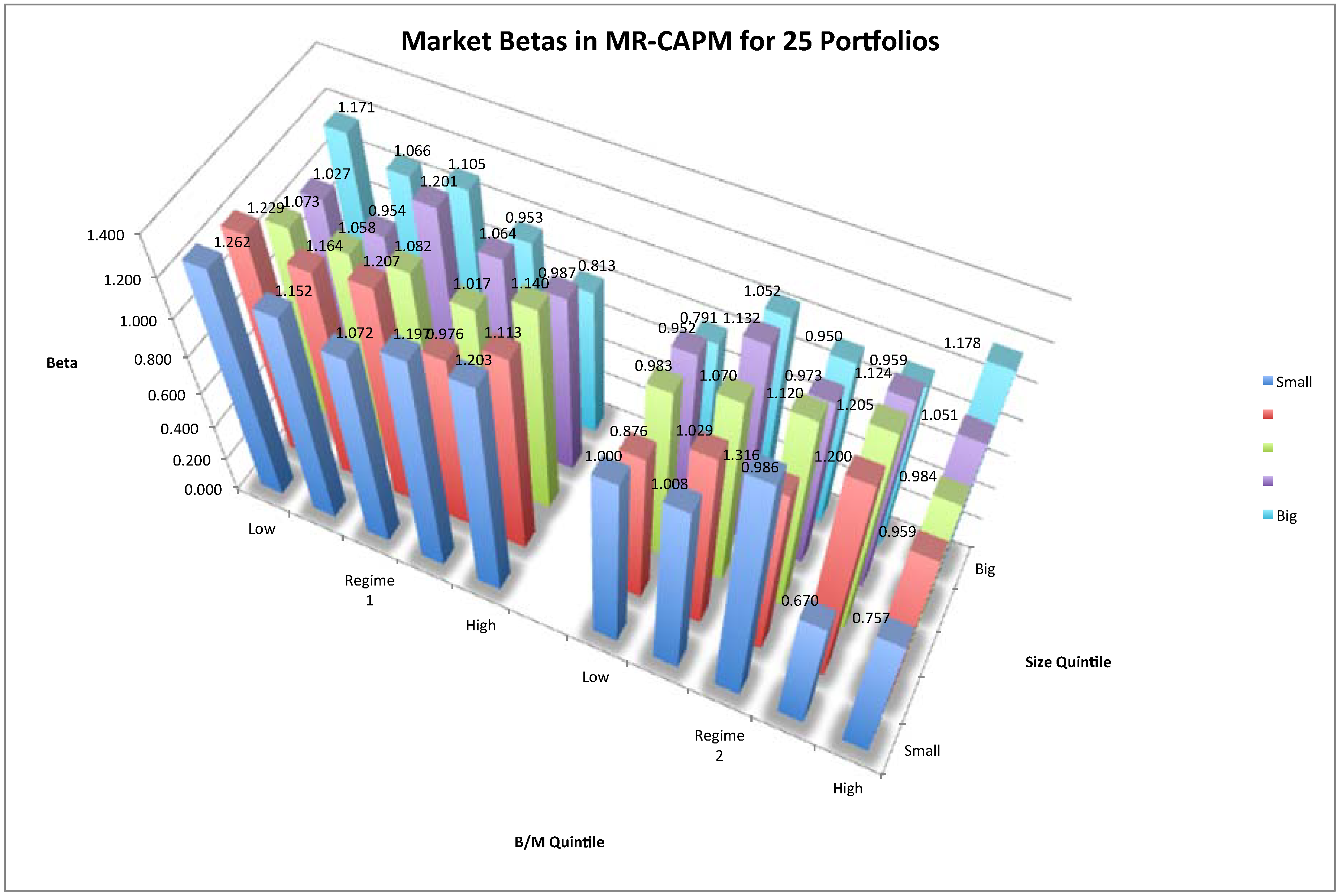
Figure 3.
Risk premium series and smoothed regime probabilities in MR-CAPM. Notes: The figure shows the conditional means of risk premiums and the smoothed probability of being either a bear market (red area) or a bull market (green area). The observation period is from July 1995 to March 2015.
Figure 3.
Risk premium series and smoothed regime probabilities in MR-CAPM. Notes: The figure shows the conditional means of risk premiums and the smoothed probability of being either a bear market (red area) or a bull market (green area). The observation period is from July 1995 to March 2015.

Figure 4.
Market betas in MR-FF3 for 25 size-B/M portfolios. Notes: The three-dimensional space shows the market betas in the two-regime MR-FF3 for 25 size-B/M portfolios. The left group plots estimates of regime 1 and the right subfigure plots those of regime 2. The vertical axis denotes risk betas. The horizontal space denotes the 25 portfolios. The horizontal axis denotes the B/M value magnitude. From left to right, the B/M value of portfolios increases. The depth axis refers to size magnitude. As depth increases, the size of portfolios increases.

Figure 5.
SMB betas in MR-FF3 for 25 size-B/M portfolios. Notes: The three-dimensional space shows the SMB betas in the two-regime MR-FF3 for 25 size-B/M portfolios. The right group plots estimates of regime 1 and the left subfigure plots those of regime 2. The vertical axis denotes risk betas. The horizontal space denotes the 25 portfolios. The horizontal axis denotes the B/M value magnitude. From right to left, the B/M value of portfolios increases. The depth axis refers to size magnitude. As depth increases, the size of portfolios decreases.

Figure 6.
HML betas in MR-FF3 for 25 size-B/M portfolios. Notes: The three-dimensional space shows the HML betas in the two-regime MR-FF3 for 25 size-B/M portfolios. The right group plots estimates of regime 1 and the left subfigure plots those of regime 2. The vertical axis denotes risk betas. The horizontal space denotes the 25 portfolios. The horizontal axis denotes the B/M value magnitude. From right to left, the B/M value of portfolios increases. The depth axis refers to size magnitude. As depth increases, the size of portfolios decreases.

Figure 7.
One-Step-Ahead forecasting of an MR-FF3 model. Notes: The figure illustrates the expanding estimation window and the forecasting window of an out-of-sample analysis for an MR-FF3 model.
Figure 7.
One-Step-Ahead forecasting of an MR-FF3 model. Notes: The figure illustrates the expanding estimation window and the forecasting window of an out-of-sample analysis for an MR-FF3 model.

Figure 8.
Out-of-sample forecasting return vs. actual return for each portfolio. Notes: The figure depicts the one-step-ahead, out-of-sample forecasting returns (red line) and actual monthly returns (blue line), during the period from April 2015 to December 2017 for the 1st, 5th, 21st, and 25th of the Fama–French 25 portfolios (P01, P05, P21, P25).
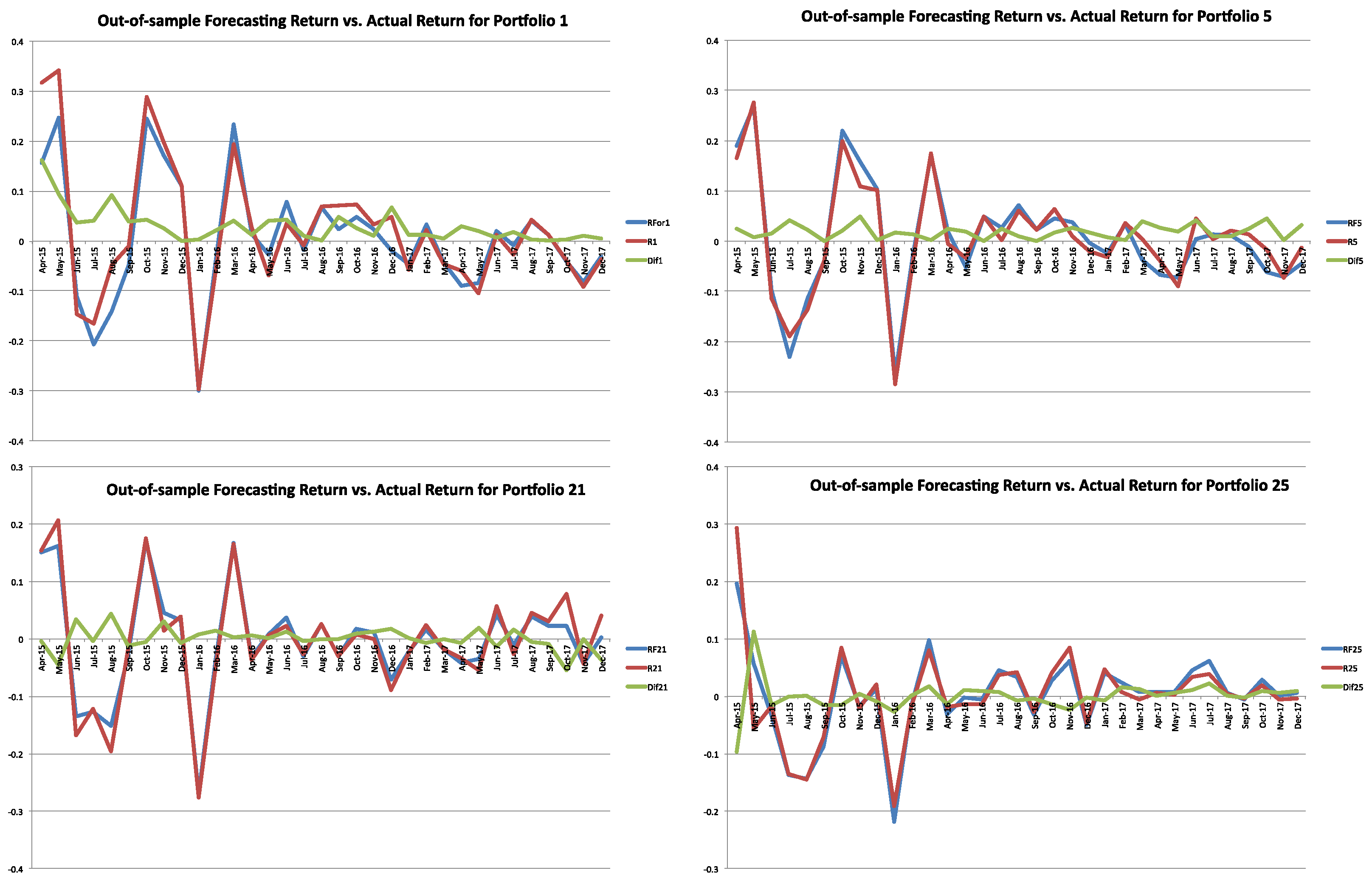
Figure 9.
Average out-of-sample forecasting return vs. actual return. Notes: The figure depicts the one-step-ahead, out-of-sample forecasting returns (denoted by Avg Forecast), actual monthly returns (denoted by AvgTrue), and their differences (denoted by Diff), during the period from April 2015 to December 2017 for the Fama–French 25 portfolios.


Table 1.
Formation of common risk factors.
| Size | Book-to-Market (B/M) | ||
|---|---|---|---|
| Growth | Medium | Value | |
| (30%) | (40%) | (30%) | |
| Small (50%) | S/L | S/M | S/H |
| Big (50%) | B/L | B/M | B/H |
Note: Size refers to the market capitalization of the stocks in June year t. Book-to-Market (B/M) is the book equity of last fiscal year-end in December divided by market value for December, year t – 1. “L”, “M”, and “H” represent the low, medium, and high B/M levels, respectively. All of the stocks were sorted based on size and B/M cutoffs. Six groups were formed, denoted as “S/L”, “S/M”, “S/H”, “B/L”, “B/M”, and “B/H”.
Table 2.
Parameter estimates of the MR-CAPM.
| Regime | St = 1 (Bear) | St = 2 (Bull) | |
|---|---|---|---|
| Transition matrix Π | St = 1 (Bear) | 0.97 (0.00) | 0.06 (0.00) |
| St = 2 (Bull) | 0.03 (0.00) | 0.94 (0.00) | |
| Expected Duration | 34.05 | 18.01 | |
| MKT | μm | −0.005 (0.38) | 0.048 (0.00) |
| σm | 0.059 (0.00) | 0.122 (0.00) | |
Note: This table reports the estimates of parameters in the two-state MRS model developed in Section 2.2.2. The p-values are reported in the parentheses under the corresponding mean. Π is the state transition matrix, which reports the probability of switching from one state to another. The sample period is from July 1995 to March 2015, on a monthly basis.
Table 3.
Parameter estimates of the MR-FF3 model.
| Regime | St = 1 (Bear) | St = 2 (Bull) | |
|---|---|---|---|
| Transition matrix Π | St = 1 (Bear) | 0.95 (0.00) | 0.11 (0.00) |
| St = 2 (Bull) | 0.05 (0.00) | 0.89 (0.00) | |
| Expected Duration | 18.89 | 9.36 | |
| MKT | μm | −0.001 (0.85) | 0.037 (0.02) |
| σm | 0.060 (0.00) | 0.123 (0.00) | |
| SMB | μs | 0.009 (0.01) | 0.008 (0.28) |
| σs | 0.031 (0.00) | 0.057 (0.00) | |
| HML | μh | 0.004 (0.28) | 0.003 (0.65) |
| σh | 0.027 (0.00) | 0.003 (0.00) | |
Note: This table reports the estimates of parameters in the two-state MRS model developed in Section 2.2.3. The p-values are reported in the parentheses under the corresponding mean. Π is the state transition matrix, which reports the probability of switching from one state to the other. The sample period is from July 1995 to March 2015 on a monthly basis.
Table 4.
Time-series regressions of “5–21” portfolio returns on risk factors.
| Panel A: Estimates for the Four Models | |||||
| Model | Regime | Intercept | MKT | SMB | HML |
| Unconditional CAPM | 0.011 | 0.061 | |||
| (0.038) | (0.303) | ||||
| MR-CAPM | St = 1 | 0.010 | 0.161 | ||
| (0.006) | (0.000) | ||||
| St = 2 | 0.017 | −0.052 | |||
| (0.223) | (0.698) | ||||
| Unconditional FF3 | −0.002 | −0.004 | 1.436 | 1.437 | |
| (0.301) | (0.868) | (0.000) | (0.000) | ||
| MR-FF3 | St = 1 | −0.004 | 0.031 | 1.439 | 1.235 |
| (0.010) | (0.091) | (0.000) | (0.000) | ||
| St = 2 | 0.018 | −0.183 | 1.042 | 2.105 | |
| (0.076) | (0.067) | (0.000) | (0.000) | ||
| Panel B: Statistics for the Four Models | |||||
| Model | SSR | Log Likelihood | AIC | BIC | HQC |
| Unconditional CAPM | 1.470 | 266.017 | −2.228 | −2.199 | −2.216 |
| MR-CAPM | 1.472 | 313.237 | −2.576 | −2.459 | −2.529 |
| Unconditional FF3 | 0.222 | 489.909 | −4.100 | −4.042 | −4.077 |
| MR-FF3 | 0.179 | 544.315 | −4.492 | −4.317 | −4.421 |
Note: This table reports the parameter estimates and statistics for the unconditional CAPM, MR-CAPM, unconditional FF3 model, and MR-FF3 model. Excess returns of a “5–21” hedging portfolio are regressed on the risk factor premiums. The sample period is from July 1995 to March 2015 on a monthly basis. p-values are reported in the parentheses under the corresponding estimates. SSR is the sum of squared residuals. AIC refers to Akaike information criterion, while BIC refers to Schwarz criterion, and HQC denotes Hannan–Quinn information criterion.
Table 5.
Performance of the MR-FF3 in in-sample and out-of-sample fitting.
| MR-FF3 | In-Sample RMSE | Out-of-Sample RMSE |
|---|---|---|
| 1995.07–2015.03 | 2015.04–2017.12 | |
| Portfolio 1 | 0.045 | 0.039 |
| Portfolio 5 | 0.034 | 0.019 |
| Portfolio 21 | 0.027 | 0.020 |
| Portfolio 25 | 0.027 | 0.020 |
| Hedging Portfolio of “5–21” | 0.027 | 0.016 |
Note: This table reports the performance of the MR-FF3 model in in-sample and out-of-sample fitting. Results of portfolio 1, 5, 21, and 25 of the FF25 portfolios and a “5–21” hedging portfolio are reported. The in-sample period spans from July 1995 to March 2015, while the out-of-sample period is from April 2015 to December 2017, on a monthly basis. RMSE is the Root Mean Squared Error.
© 2018 by the authors. Licensee MDPI, Basel, Switzerland. This article is an open access article distributed under the terms and conditions of the Creative Commons Attribution (CC BY) license (http://creativecommons.org/licenses/by/4.0/).
Share and Cite
MDPI and ACS Style
Chen, J.; Kawaguchi, Y. Multi-Factor Asset-Pricing Models under Markov Regime Switches: Evidence from the Chinese Stock Market. Int. J. Financial Stud. 2018, 6, 54. https://doi.org/10.3390/ijfs6020054
AMA Style
Chen J, Kawaguchi Y. Multi-Factor Asset-Pricing Models under Markov Regime Switches: Evidence from the Chinese Stock Market. International Journal of Financial Studies. 2018; 6(2):54. https://doi.org/10.3390/ijfs6020054
Chicago/Turabian StyleChen, Jieting, and Yuichiro Kawaguchi. 2018. "Multi-Factor Asset-Pricing Models under Markov Regime Switches: Evidence from the Chinese Stock Market" International Journal of Financial Studies 6, no. 2: 54. https://doi.org/10.3390/ijfs6020054
Note that from the first issue of 2016, this journal uses article numbers instead of page numbers. See further details here.