1. Introduction
The influence of taxation on the willingness of firms and individuals to invest is one main topic in the tax literature.
1 For example, the effects of introducing or increasing an income tax or a capital gains tax, loss offset provision, asymmetric taxation of gains and losses or asymmetric taxation of different investment opportunities or investor groups are only some central issues of this strand of literature. Additionally, accounting principles, such as depreciation regulations, are important aspects that influence the advantageousness of investment alternatives as they alter the net present value of these opportunities by means of affecting the tax base and, therefore, the tax amount in each period over the time horizon.
Our aim is to study how depreciation rules—namely straight-line and accelerated depreciation—influence the decision behavior of investors. For this purpose, we conduct a laboratory experiment in which participants decide on the composition of an asset portfolio in different choice situations. To induce an investment environment in the lab that is closer to reality, we decided that subjects receive their money from the experiment not only immediately after the experiment has finished, but also after a certain time-lag. This enables us to study the behavior of investors when they are confronted with an investment decision over different time periods. Therefore, we are able to analyze the timing/interest effects of different depreciation rules on the willingness to invest in a controlled environment. So far, there is no study in the tax and accounting literature that applies such an experimental setting to investigate this research question.
In addition to studying these depreciation effects, one further objective of our study is to replicate the finding of [
3]. They find that introducing a subsidy (and consequently making the decision environment more complex) leads to a lower willingness to take risks, although the net returns are kept constant. With our study, we will replicate this result in a completely other experimental setting, which underscores the importance of their finding. Furthermore, and beyond the observation of [
3], we will show that investors’ response to an accelerated depreciation rule depends on whether a subsidy is introduced or not.
The findings of our study are manifold. First, we find that an accelerated compared to a straight-line depreciation rule increases the willingness to invest as hypothesized by theory in our more complex treatment with a subsidy. However, in our less complex treatment without subsidy, this expected behavior is not observed. Second, we are able to replicate the findings observed by [
3] when the time-lag between the payment periods is not too long. Third, we show that tax misperception biases do not occur when comparing the straight-line and accelerated depreciation rule. Fourth, our study indicates that experimental results depend to some extent on the experimental environment and raises, therefore, new questions for future research analyzing why these environment-dependent differences occur.
The remainder of the paper is organized as follows: In
Section 2, we give a brief review of the theoretical, empirical and experimental literature. In
Section 3, we present the design of our experiment and formulate our hypotheses. The results of our study are given in
Section 4. The results of a variation treatment as a robustness check are presented in
Section 5. In our last
Section 6, we summarize and discuss our findings.
2. Literature Review
The research question of how depreciation regulations influence the investment behavior of firms and individuals has been discussed in the theoretical and empirical tax literature for many decades.
2 Wakeman [
5] formally proves that accelerated depreciation is preferred to straight-line depreciation for every positive discount rate, as the present value of the asset’s positive cash flows in the first period will surpass that of the negative cash flows in the second period. However, this finding is restricted by several assumptions that are implicitly made: the existence of certain cash flows, a linear and time-constant tax system and the restriction not to switch between both depreciation methods. Therefore, many studies have revealed that straight-line depreciation may be optimal if at least one of these assumptions is not met. First, [
6,
7,
8] formally prove that straight-line depreciation might be preferred if future cash flows are uncertain. Determining the optimal depreciation scheme that minimizes future tax payments, [
8] show that the degree of uncertainty in future cash-flows largely affects the optimal depreciation choice. In this context, [
6] show that the straight-line depreciation method is favored for lowering the company’s present value of tax liability if the future cash flow is uncertain or if the company is not allowed to carry forward losses for tax purposes and the discount factor for future tax payments or future cash flows is high. Second, besides the influence of the discount factor and the degree of uncertainty of future cash flows, [
7] reveal that also the structure of the tax system influences the preference of a depreciation method. Hence, under progressive tax systems, straight-line depreciation might be favored if there are stable or growing future cash flows. In this regard, [
9] demonstrate that while the accelerated depreciation provides discounting benefits, straight-line depreciation is advantageous under a progressive tax system. Third, [
10] analyze whether straight-line depreciation is also used if tax authorities allow switching the depreciation method. They find that this option’s value depends on the discount factor, the probability that proposed depreciation changes are accepted and whether loss carry forward is allowed. Concerning loss carry forward opportunities, [
11] model conditions in which straight-line depreciation is favored over accelerated depreciation if periods of consecutive losses exceed a threshold that is determined by the allowable periods to carry a loss forward.
Coen [
12] derives two ways in which the accelerated depreciation, compared to the straight-line depreciation, can stimulate investments: an accelerated depreciation increases (1) the after-tax rate of the return on the asset (“rate-of-return effect”) and (2) the cash flows (“liquidity effect”). Coen [
12] estimates the tax savings for 1954–1966 resulting from the accelerated depreciation and the investment tax credit. He finds that the stimulus based on the accelerated depreciation is always higher than the stimulus based on the tax credit. Klein and Taubman [
13] build up an econometric model and estimate the effect of accelerated depreciation and the investment tax credit on investments based on several U.S. investment data. They examine the consequences of a temporary suspension of the tax credit and the accelerated depreciation from the fourth quarter 1966 through the third quarter 1968. The results indicate that investors anticipate the suspension and delay investments. Cummins and Hassett [
14] use firm panel data to investigate the impact of changes in the costs of capital and its influence on investment decisions. For this purpose, they consider the tax reform act of 1986 in the U.S. with which the investment tax credit was exposed and depreciation lifetimes were extended. They find a strong linkage between investment decisions and the cost of capital. Increased costs of capital, as a result of, for example, increasing depreciation lifetimes, reduce investments.
Cohen et al. [
15] investigate a change in the U.S. tax law introduced with the 2002 tax bill: the introduction of a bonus depreciation allowed for a limited period of time to stimulate investments during the crisis. In particular, firms were allowed to immediately deduct an additional 30 percent of investment purchases in the first year. The remaining part has to be depreciated under standard depreciation schedules. Cohen et al. [
15] explore the impact of the 30 percent first-year deduction on the marginal cost of equipment investment. They find that this act can increase the incentive to invest in equipment markedly. House and Shapiro [
16] deal with the same change in the U.S. tax rules. They estimate the investment supply elasticity after the 30 percent first-year deduction rule was implemented. They argue that the elasticity of investments for long-lived capital goods is nearly infinite, and therefore, tax subsidies should be fully reflected in the investment prices. The result of their work indicates that the introduced immediate depreciation increases the price of the supported assets. Therefore, the investments in qualified capital increased. In addition to this tax law change in 2002, [
17] further analyze the 2003 Tax Act and its incentive effect of bonus depreciations on investments. In fact, qualified properties bought during the period from 11 September 2001 to December 2004 are subject to an extraordinary bonus depreciation of 30% and 50%, respectively. In contrast to the previous studies, they find only a weak impact of these incentives on capital spending. In line with this result, [
18] show that the accelerated depreciation method has almost no important effect on the investment behavior. Furthermore, [
19] provide additional evidence that the effectiveness of bonus depreciation is limited. Consequently, empirical studies observe mixed results regarding the investment stimulating effects of accelerated depreciation rules (see also [
20]).
Up to now, only [
21] analyze the effects of depreciation rules on investment behavior experimentally. In particular, they investigate the influence of introducing accelerated depreciation rules and tax credits on the demand for depreciable assets in a market setting. They find that the impact of the tax incentives is rather modest as they observed that the demand was unresponsive to the tax incentives. As stated by the authors, “this result is inconsistent with extant neoclassical theory and the expectations of policymakers” ([
21], p. 509).
A small, but growing literature analyzing tax perception issues finds that investment decisions can be heavily biased by a misperception of tax effects that possibly could explain the unexpected result of [
21].
3 Fochmann et al. [
43,
44], for example, investigate the willingness to take risks when an income tax with a loss offset provision is applied compared to when no taxation is applied. They observe an unexpected high willingness to take a risk under an income tax, although the gross payoffs are adapted in such a way that both settings (with and without tax) are identical in net terms, and thus, the same decision pattern was expected. In contrast, [
45] find that introducing an income tax with or without a full loss offset provision leads investors to reduce their willingness to take risks, although the gross investments are adjusted accordingly to achieve identical net investments. Ackermann et al. [
3] study how taxes and subsidies influence investment behavior. They find that, although the net income is held constant again, individuals invest less in the risky asset when a tax has to be paid or when a subsidy is paid. They conduct different variations of their baseline experiment to examine how robust these findings are and observe that only a reduction of the environment complexity by reducing the number of states mitigates the identified perception bias. The results of all of these studies show that individuals often do not react to taxation as is expected by neoclassical theory, which assumes that individuals maximize their net payoffs. Although this strand of literature does not focus on the perception of depreciation rules explicitly, these findings indicate that perception biases are possibly important, as well, when tax effects of different depreciation rules, such as straight-line or accelerated depreciation rules, on investment decisions are discussed economically. Thus, the aim of this study is to investigate both this literature on tax perception and the “standard” research literature on depreciation rules.
3. Experimental Design, Treatments and Hypotheses
3.1. Decision Task
In our setting, subjects have to decide on the composition of an asset portfolio in different choice situations.
4 At the beginning of each situation, each subject receives an endowment of 800 Lab-points where 2 Lab-points correspond to 1 Euro cent. The participants’ task is to spend their endowment on two investment alternatives: Asset A and Asset B. The price for one asset of either type is 8 Lab-points. As an investor is not allowed to save his or her endowment, he or she buys 100 assets in each decision situation in total.
The return of Asset A is risky and depends on the state of nature. Three states (good, middle, bad) are possible, and each state occurs with an equal probability of 1/3. The return of Asset B is risk-free and is therefore equal in every state of nature. The returns of both assets are chosen in such a way that Asset A does not dominate Asset B in each state of nature, but that the expected return of Asset A exceeds the risk-free return of Asset B. The subjects know the potential returns on both assets in each state of nature before they make their investment decision.
An investment in Asset A or B exactly leads to two payoffs with a time-lag between both payment dates. Subjects immediately receive the first payoff in cash after the experiment has finished. The second payoff is paid in three weeks.
5 To receive the delayed payment, a participant could choose either to come to the experimenter’s office or the experimenter transfers the money to his or her bank account. For reasons of simplification, we use “periods” instead of “payment dates” in the following. However, subjects only decide on their investment in the first period. No further decision is made in Period 2.
3.2. Income Taxation, Subsidization and Treatments
The income from Asset A is taxed at a rate of 50%. The tax base is given by the gross return resulting from Asset A (i.e., the chosen number of Asset A times the gross return per Asset A) minus the depreciation amount (dependent on the amount initially invested in Asset A). The tax is raised in each period separately. As the gross return per Asset A and the depreciation amount can be different in both periods, the tax base, the tax amount and the net payoff can differ, as well. The gross returns of Asset A are chosen in such a way that the tax base cannot be negative. The risk-free Asset B is not subject to taxation.
In our experiment, we use a 2 × 2 design in which we vary the depreciation rule (within-subject design) and the existence of a subsidy (between-subject design).
6 Thus, we have four different treatments in total. With respect to the depreciation method, we use two different rules: straight-line and accelerated depreciation. In the treatments with the straight-line depreciation rule, the total amount invested in Asset A (i.e., the chosen number of Asset A times the price of eight Lab-points for one Asset A) is equally distributed across both periods. In the treatments with the accelerated depreciation rule, the total amount invested in Asset A is completely depreciated in the first period (immediate write-off). In the second period, no further depreciation reduces the tax base.
7 Subjects are randomly assigned to the between-subject design treatments.
Regarding the subsidization, we implement treatments with and without a subsidy. In the treatments without subsidy, the decision situation is exactly as described. In the treatments with subsidy, a subsidy of two Lab-points is paid for each Asset A. For reasons of simplification, we decided that the subsidy amount does not influence the tax base and is, therefore, not taxed. The risk-free Asset B is not subsidized.
Table 1 gives an overview over all four treatments.
Table 2 exemplarily presents possible states of natures, while
Table 3 shows an example for each treatment and for each period. Please notice that this example was also used in the instructions presented to the participants, but not in the actual experiment again. In
Appendix B, the (potential) gross and net returns of both assets used in this experiment are displayed for each treatment and each (randomized) decision situation.
3.3. Hypotheses
3.3.1. Straight-Line vs. Accelerated Depreciation
As only the risky Asset A is taxed in our experiment, the applied depreciation rule only influences the after-tax return of the Asset A investment. In particular and in accordance with [
5], an accelerated depreciation leads to a higher present value of the depreciation tax shield compared to a straight-line depreciation because the depreciable amount is higher in the first period under an accelerated depreciation (timing/interest effect). Although previous literature
8 has proven mathematically that straight-line depreciation may be preferable if future cash flows are uncertain, loss carry forwards are allowed beyond a threshold, the taxpayer underlies a progressive tax system and he or she is allowed to switch between depreciation methods, our experimental design ensures that accelerated depreciation is favored. Although future cash flows are uncertain due to the three different states of nature, we exclude negative cash flows so that neither uncertainty nor loss carry forwards are decisive. Additionally, we provide a flat tax rate and do not allow switching between the depreciation methods. As a consequence, this leads to a higher net present value of the Asset A investment under an accelerated than under a straight-line depreciation. Thus, in accordance with the theoretical literature, we hypothesize that an accelerated compared to a straight-line depreciation leads to a higher willingness to invest in the risky Asset A. This leads us to our first hypothesis.
9Hypothesis 1. The investment in the risky Asset A is higher under an accelerated than under a straight-line depreciation.
Different experimental studies have found tax perception biases that contradict theoretical predictions (see
Section 2). However, no study analyzes whether such biases occur in the context of depreciations. From this perspective, we can formulate no clear hypothesis. Nevertheless, some studies give evidence that a perception bias could matter in this context. Since in the case of a straight-line depreciation the asset is depreciated over a longer time horizon than in the case of an accelerated depreciation rule, the associated complexity level is possibly higher in the former than in the latter. In line with the findings [
32,
34,
35,
36,
37], this could lower the quality of investment decisions and consequently could increase the likelihood of observed decision biases in the case of a straight-line depreciation. Furthermore, [
43,
44] show that the possibility to deduct losses can have an unexpected positive effect on investment behavior. As the depreciation of an asset has the same deducting effect as losses (i.e., in both cases, the tax base is reduced), such tax perception biases may occur in the depreciation context, as well. The question of whether different depreciation rules have asymmetric effects on the willingness to invest beyond theoretically-expected effects is of political importance. If a systematic difference can be proven, the government could, by applying a certain depreciation rule, enhance investment behavior (more than theoretically predicted).
We implement net and gross value equivalence decision situations in our experiment. See
Table 4 and
Table 5 for examples (see also
Table B1 and
Table B2 in the
Appendix B). In the gross value equivalence decision situations, all gross payoffs are identical across the treatments with straight-line and accelerated depreciation. These decision situations are used to test Hypothesis 1. To isolate tax perception biases, we use the net value equivalence decision situations. In these decision situations, the gross payoffs in each treatment are adapted in such a way that the net payoffs are identical across the treatments. Thus, in net terms, the choice situations are completely identical in all of our treatments in these decision situations. Consequently, the same decision pattern is expected in all treatments when no perception bias occurs. Since we cannot formulate a specific prediction, we use the null hypothesis as our Hypothesis 2:
Hypothesis 2. If the net returns are identical, investment in the risky Asset A and the risk-free Asset B is identical irrespective of whether an accelerated or a straight-line depreciation is applied.
For each of the two depreciation rules, we use five net and five gross value equivalence decision situations, respectively. Hence, each subject is confronted with 20 decision situations in total.
Table 6 depicts this procedure. To avoid any order effects, the sequence of these 20 decision situations is randomized for each participant.
3.3.2. Subsidy vs. No Subsidy
Ackermann et al. [
3] show that introducing a subsidy while keeping the net returns constant leads to an unexpected perception bias that results in a reduced willingness to take risks. As discussed by [
3], one explanation for this result could be that introducing a subsidy results in a more complex decision environment, leading investors to decrease their willingness to take risks. A similar observation that points in this direction can be found in [
45]. To analyze this perception bias, we use two treatments with and without subsidy, but adapt the gross returns in such a way that the net returns are identical in both treatments.
10 Following the observation of [
3], we conjecture:
Hypothesis 3. If the net returns are identical, investment in the risky Asset A is lower with than without subsidy.
3.4. Experimental Protocol
The experiment was conducted at the computerized experimental laboratory of the Otto-von-Guericke University of Magdeburg (MaXLab). In total, 165 subjects
11 (62 females and 103 males) participated and earned on average 12.91 Euros in approximately 100 minutes (about 7.75 Euros per hour). The experimental software was programmed with z-Tree ([
52]), and subjects (mainly economic students) were recruited with the Online Recruiting System for Economic Experiment (ORSEE) ([
53]).
We implement different methods to make sure subjects understand the decision environment. First, at the beginning of the experiment, the instructions are read out loudly where the procedure of the experiment and the payoff mechanism are explained to the participants. The instructions contain a numerical example for each depreciation rule and for each payment date. In this example the calculation of the net payoff resulting from Assets A and B, as well as the total net payoff are explained. The participants have time to read the instructions for their own and to ask questions. Second, after reading the instructions, participants face a comprehension test in which they are confronted with a similar example as given in the instructions, but with new numerical values. The test is solved after all questions are answered correctly. Third, participants receive a pocket calculator, which could be used during the whole experiment for their own calculations. Fourth, a “what-if-calculator” is provided in each decision situation, which allows subjects to calculate their tax burden, the (net) payoff resulting from Assets A and B and the total net payoff at different investment levels.
To avoid income effects and strategies to hedge the risk across all decision situations, only one of the 20 decision situations is paid out. For this purpose, each participant is asked to randomly draw a number from 1–20 at the end of the experiment to select his or her payoff relevant decision situation. Hereafter, the participant has to cast a six-sided die to determine the relevant state of nature. The state of nature is good, middle and bad if the number is 1 or 2, 3 or 4 and 5 or 6, respectively. Dependent on the chosen quantities of Assets A and B in the selected decision situation, the participant’s payoffs are calculated for each of the two periods, and the payoff of the first period is paid out immediately in cash.
4. Results
4.1. Straight-Line vs. Accelerated Depreciation
For our statistical analyses, we use the share of endowment invested in the risky Asset A as our dependent variable. The amount invested in the risk-free Asset B is the residual share.
Table 7 presents descriptive statistics for our dependent variable separated for the treatments and for the gross and net value equivalence decision situations. To analyze our treatment differences statistically, we use the non-parametric Mann-Whitney U test (MWU) and the parametric
t-test both for two independent samples.
Table 7 shows the resulting (two-sided)
p-values of both tests when we compare the straight-line and accelerated depreciation treatment.
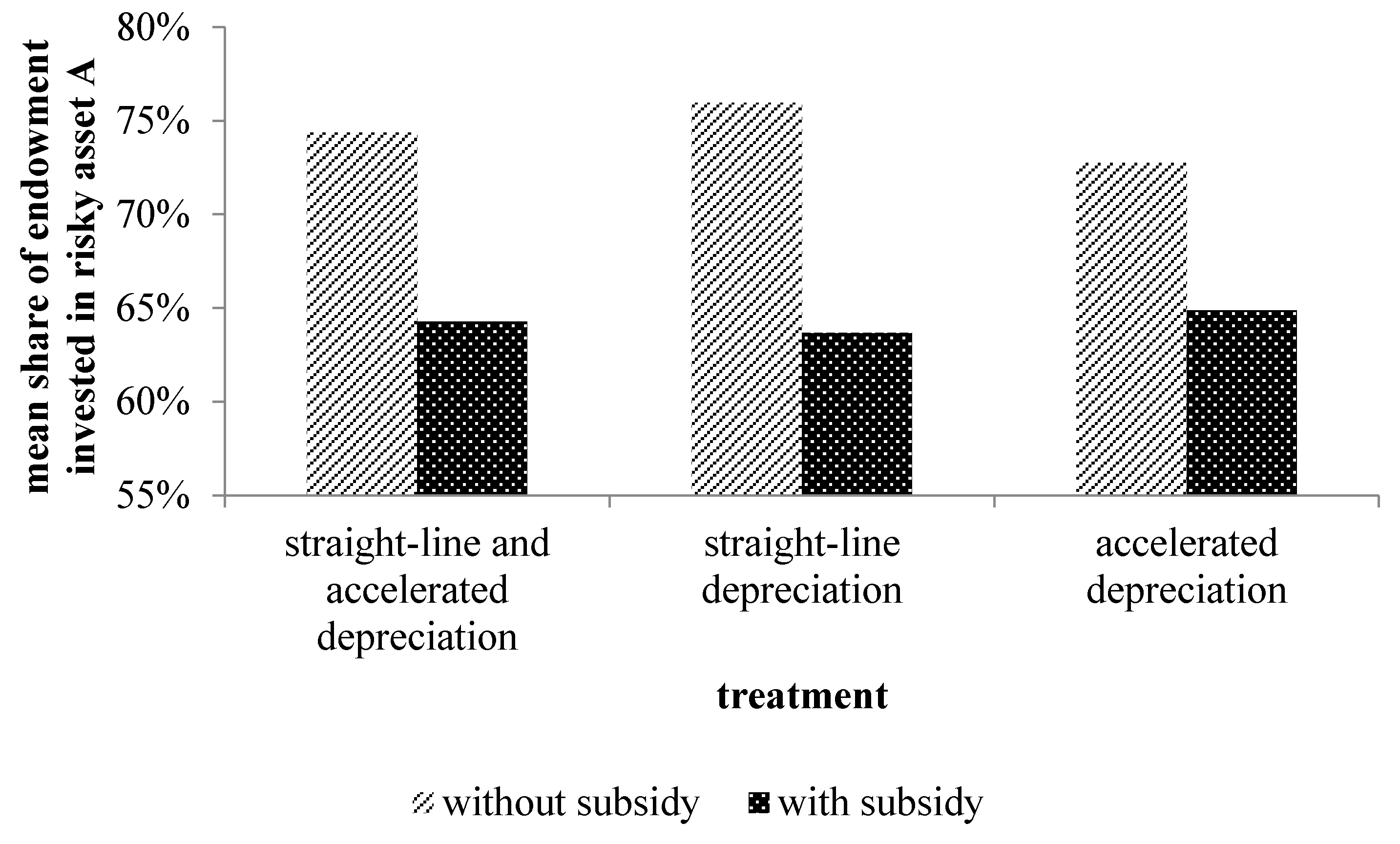
Figure 1 depicts the mean share of endowment invested in the risky Asset A.
In the gross value equivalence decision situations, we expect a higher willingness to invest in the risky asset under an accelerated than under a straight-line depreciation (Hypothesis 1). In the treatment with subsidy, this investment behavior is actually observed, and both statistical tests indicate a significant difference between both depreciation treatments (p-values below 5%). Thus, Hypothesis 1 can be confirmed. In the treatment without subsidy, however, we do not observe the expected decision pattern, and the differences are not statistically significant (p-values above 10%). As a result, Hypothesis 1 has to be rejected for the case without subsidy.
With respect to the net value equivalence decision situations, we hypothesize that the same investment behavior as the net returns to be identical in both depreciation treatments (Hypothesis 2). Independent of whether a subsidy is paid or is not paid, we observe no economically and statistically significant difference between the straight-line and accelerated depreciation treatment. All p-values are above the 10% level. This result is in accordance with Hypothesis 2, which we can therefore confirm.
In addition to our bivariate analyses, we run random-effects linear regressions and cluster standard errors on the subject level. This analysis meets three requirements: First, multivariate analysis allows controlling for further independent variables simultaneously. Second, linear regressions that cluster observations at the subject level account for the dependence of observations as one subject makes 20 decisions, which are therefore not independent of each other. Third, the random effects model is used to account for the observations’ dependence while allowing independent variables to be constant within the 20 decisions for the same subject (e.g., age). The results are presented in
Table 8.
Models 1a and 1b, as well as Models 2a and 2b present the regressions’ results for decisions made without subsidy. Models 3a and 3b, as well as Models 4a and 4b present regressions’ results for decisions made where a subsidy is provided. Models 1a and 1b, as well as Models 3a and 3b (2a and 2b, as well as 4a and 4b) present the regressions’ results for gross value equivalence decision situations (net value equivalence decision situations). While Models 1a, 2a, 3a and 4a only test the influence of the depreciation method on risk taking, Models 1b, 2b, 3b and 4b also control for socio-demographic variables. As before, the dependent variable measures the share of endowment invested in the risky Asset A. Straight-line depreciation is a dummy variable that denotes whether the decision is made under straight-line or accelerated depreciation. It takes the value one if the decision is made under straight-line depreciation and zero, otherwise. Age denotes the subject’s age in years. Male (Economics and Management) takes the value one if the subject is male (studies at the Faculty of Economics and Management) and zero if the subject is female (studies at any other faculty).
We can confirm the results we have obtained in the bivariate analysis. In the gross value equivalence decision situations, we expect a higher willingness to invest in the risky asset under an accelerated than under a straight-line depreciation (Hypothesis 1). However, we can only confirm this hypothesis if a subsidy is granted (p-values of 0.035 and 0.036 in Models 3a and 3b, respectively). In the case without a subsidy, Hypothesis 1 has to be rejected. Analyzing the net value equivalence decision situations, we expect to find no differences in the investment behavior for both depreciation rules (Hypothesis 2). As for Models 2a and 2b, as well as for Models 4a and 4b, we do not find any significant differences in the investment behavior, we can confirm Hypothesis 2. Generally, the control variables have no significant influence on the investment decision.
4.2. Subsidy vs. No Subsidy
As observed by [
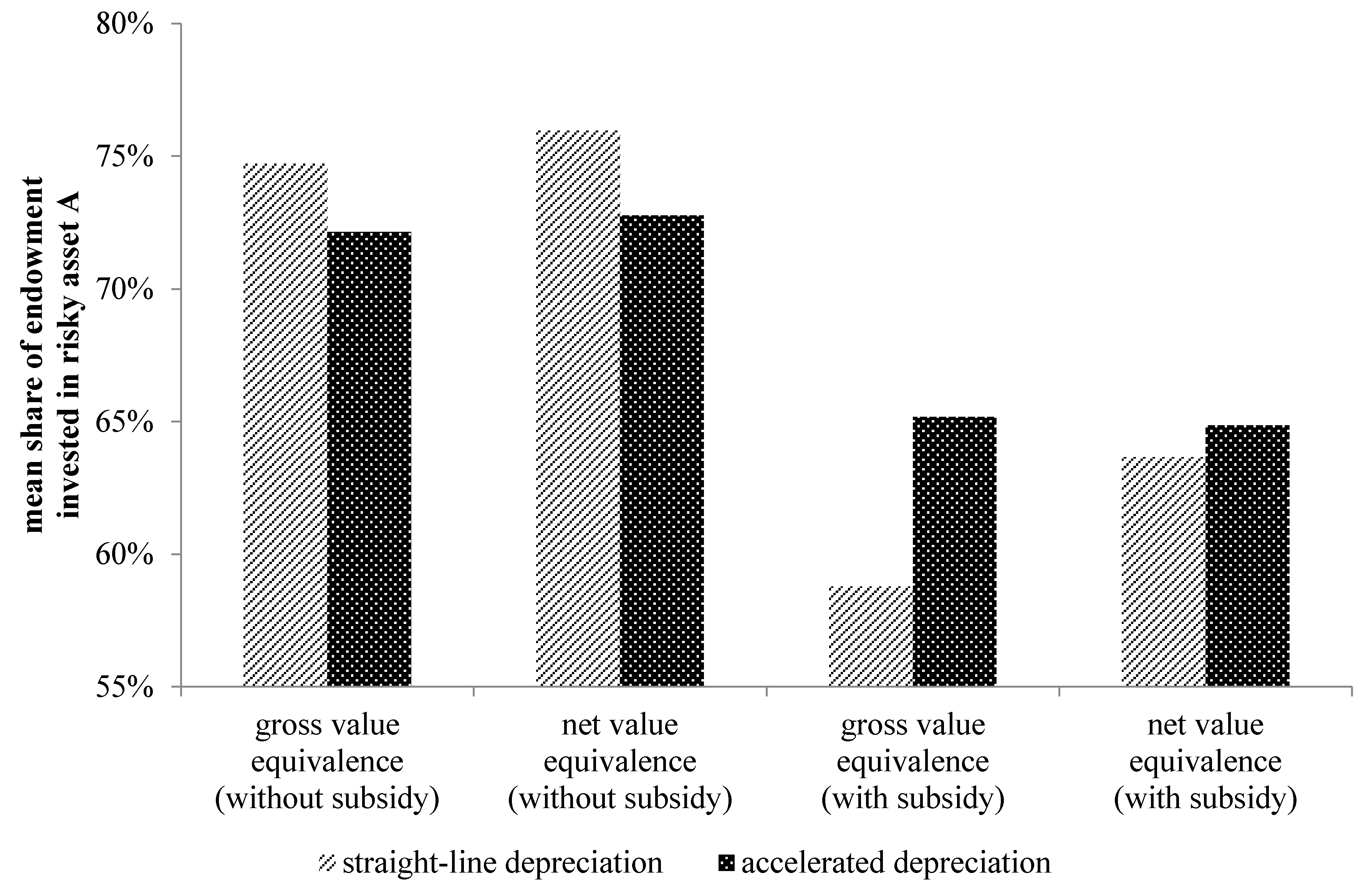
3], we hypothesize that introducing a subsidy leads investors to reduce their willingness to invest in the risky Asset A, although the net returns are not affected by this subsidy (Hypothesis 3). As we are only interested in the decision situations with identical net returns, we just focus on the results of the net value equivalence decision situations in the following.
Table 9 presents different descriptive statistics, and
Figure 2 depicts the mean share of endowment invested in the risky Asset A. Independent of whether we aggregate the results from both depreciation treatments or not, we observe that the willingness to invest in the risky Asset A decreases markedly when a subsidy is paid. All differences are statistically significant (at least) at the 5% level. Thus, Hypothesis 3 is supported, and the results of [
3] are confirmed by our study.
5. Robustness Check: Three-Month Time-Lag
In the following, we analyze how robust our results are with respect to the length of the time-lag between the first and the second period. The idea is that receiving the second payoff not in three weeks, but in, for example, three months makes the investment decision more important as individuals are perhaps more interested in earning money today and not in the distant future. Thus, we decided to extend the time-lag to three month. Everything else remains unchanged.
Table 10 and
Table 11 present descriptive statistics for the mean share of endowment invested in the risky Asset A for the treatments with the three-month time-lag.
Regarding the differences between the straight-line and accelerated depreciation treatments (see
Table 10), we observe very similar results as we observed with a time-lag of three weeks. In the gross value equivalence decision situations, we only observe an economically- and statistically-significant difference between both deprecation treatments in the treatment with subsidy. As a consequence, Hypothesis 1 has to be confirmed for the case with subsidy, but has to be rejected for the case without subsidy. In the net value equivalence decision situation, we find no differences, and therefore, Hypothesis 2 is supported, again. So far, these results are robust to different time-lags. With respect to the introduction of a subsidy (
Table 11), we still observe a decrease of the willingness to invest in the risky Asset A when a subsidy is paid. However, the difference is not significant anymore. As a consequence, Hypothesis 3 is confirmed in the three-week case, but not in the three-month case.
6. Summary and Discussion
The aim of this study is to analyze how depreciation regulations influence the decision behavior of investors. For this purpose, we conduct a laboratory experiment in which participants decide on the composition of an asset portfolio in different choice situations. In line with the theoretical literature, we hypothesize that the capital amount invested in the risky asset is higher under an accelerated than under a straight-line depreciation, as the net present value of the investment is higher in the former case (Hypothesis 1). As a result, this hypothesis is supported by our data, but only in the more complex treatment with a subsidy. If no subsidy exists, however, the hypothesis has to be rejected.
To control for perception biases, which are possibly responsible for this unexpected decision pattern, we use treatments in which the gross returns are adapted in such a way that the net returns are identical under both depreciation methods (net value equivalence decision situations). As a consequence, the same investment behavior is expected in these treatments (Hypothesis 2). In line with this hypothesis, we observe no economically- and statistically-significant difference between the straight-line and accelerated depreciation treatment irrespective of whether a subsidy is paid or not. Thus, we can summarize (1) that perception biases do not occur in this context, but (2) that the theoretical prediction that an accelerated depreciation rule spurs investments is only observed in the more complex treatment with a subsidy. These findings are robust even in a setting in which the time-lag between the first and second period is extended to three months instead of three weeks.
To replicate the unexpected observation of [
3] that introducing a subsidy leads to a lower willingness to take risks although the net returns are kept constant, we implement treatments with and without a subsidy. Independent of whether we aggregate the results from both depreciation treatments or not, we observe that the willingness to invest in the risky asset decreases markedly when a subsidy is paid. Thus, we are able to replicate the findings observed by [
3] in another kind of experimental environment with different payment periods.
Interestingly, this behavior is not significantly observed in our robustness check treatments in which the time-lag between the first and second period is extended to three months. One plausible explanation for this asymmetric behavior is that subjects take the investment decision more seriously in the three-month than in the three-week setting. In the former case, subjects are perhaps more willing to think about the choice problem, since a “wrong” decision would possibly lead to a lower payoff today and a higher payoff in the distant future. Since this trade-off of receiving less today and more in the future is more important in the three-month than in the three-week setting, a more “rational” behavior and, thus, a lower level of perception bias is to be expected in the first case.
In addition to our contribution to the literature on the effects of different depreciation methods on investment decisions, our study indicates (in line with other studies) that experimental results depend to some extent on the experimental environment. In particular, we show that the theoretically expected higher willingness to invest under an accelerated depreciation rule is only observed in the more complex treatment with a subsidy, and we show that the perception bias found by [
3] is only observed in the environment with the three-week time-lag between both payment periods. Therefore, it may be interesting for future research to analyze in more detail why these environment-dependent differences occur. One beneficial extension would be to explicitly analyze the effect of complexity on investors’ responses to depreciation rules. So far, we varied complexity only indirectly by applying a subsidy or not. However, directly varying the level of tax complexity would help to understand whether our investment-enhancing effect of an accelerated depreciation rule in the case of a subsidy is indeed driven by complexity or by another determinant that we were not able to control for. As real-world decisions are characterized by high complexity, further research is, therefore, needed to analyze the potential interaction effects of complexity and tax incentives. So far, our study only provides an indication for the existence of such effects.


