Performance of the Multifractal Model of Asset Returns (MMAR): Evidence from Emerging Stock Markets

Abstract

In this study, the performance of the Multifractal Model of Asset Returns (MMAR) was examined for stock index returns of four emerging markets. The MMAR, which takes into account stylized facts of financial time series, such as long memory, fat tails and trading time, was developed as an alternative to the ARCH family models. Empirical analysis of the study consists of two sections. In the first section, we estimated the parameters of GARCH, EGARCH, FIGARCH, MRS-GARCH and MMAR for the stock index returns of Croatia, Greece, Poland and Turkey. In the second section, 1000 paths were obtained for each model using Monte Carlo simulations. We then compared the scaling function values of simulated and original time series for different q orders (1–5). According to the obtained results, the MMAR is mostly superior to other models and presents the best replica of the original time series. Another important finding is the achievement of the MRS-GARCH. We found that for lower levels of persistency (long memory) of return series, the performance of the MRS-GARCH excels, and for H = 0.5, it narrowly outperforms the MMAR.

1. Introduction

Conventional finance theory was built on pioneering studies published in the 1950s and is based on the random walk theory and the Efficient Market Hypothesis (EMH) of [1,2]. Random walk and a normal distribution have been the assumptions of many subsequent theories that have come under heavy criticism.

Mandelbrot [3,4], who exhaustively analyzed the fat tails that were introduced to the finance literature by Vilfredo Pareto and Paul Levy, criticized conventional finance theory. He noticed that the distribution of cotton price variability has thicker tails than the normal distribution. Besides the fat tails of the return distributions, Mandelbrot and Wallis [5] demonstrated the long-range dependence property of the financial time series inspired by the study of Hurst [6] and expressed this situation as the “Joseph effect”, a references to the Bible. By means of the studies conducted by Mandelbrot, a new door was opened in finance theory regarding fractals. As stated by Taqqu [7] “Benoit’s great gift was his ability to recognize the hidden potential in certain mathematical objects”. Following Mandelbrot’s innovation in finance theory, studies in the field of fractals gained momentum. For example, Peters [8] made a great contribution to the construction of the theoretical framework of the Fractal Market Hypothesis (FMH) as an alternative to the EMH. According to this new theory, when the markets are stable, returns of financial assets present the same auto-covariance structure in different time scales, such as daily, weekly and monthly. For instance, if the daily returns exhibit positive temporary dependence, weekly and monthly returns show similar results.

Loosely speaking, fractals can be defined as iteratively-produced structures based on the self-affinity property and long memory features. Many simple fractals are self-affine geometric objects. In general terms, regardless of the scale at which they are being viewed, fractals display identical geometric patterns. An analog feature of the random geometric objects is the stochastic self-affinity. As the stochastic self-affinity is integrated in stable increments, this property is instrumental to the hyperbolic behavior of the spectral density and therefore will exhibit the long memory and non-persistent concept. Hence, the existence of the fractals constitutes the basis for the explanation of the long memory features of financial asset returns [9]. Self-affinity, the most important feature of the fractals, can be explained as follows: a process $\left\{X\left(t\right),t\in ℝ\right\}$ is self-affine for the index of $H>0$ and any $a>0$. In that case, $\left\{X\left(at\right),t\in ℝ\right\}$ has the same finite-dimensional distribution as $\left\{a^{H}X\left(t\right),t\in ℝ\right\}$. Therefore, there will be a scaling as seen in a fractal, and this process is self-affine for $0<H<1$ [7]. The self-similarity feature of any object displays its isotropic structure. This feature is not held for the time series in which dependent (price or return) and independent (time) variables are measured by different units. For these series, the self-affinity feature appears instead of self-similarity [10]. In conjunction with a suitable rescaling transformation, the self-affine return series displays a self-similarity feature. Self-affine series perform with the same distribution properties when the returns are measured in any frequency and are stated as monofractal [11]. Hence, it can be said that self-similarity is a special form of self-affinity.

Following the arguments about stylized facts seen in the financial time series, such as fat tails, volatility clustering and leverage effects, Engle [12] filled a huge gap in financial econometrics when he introduced the Autoregressive Conditional Heteroscedasticity (ARCH) model, which was based on the specifying of conditional variance. Bollerslev [13] followed with the Generalized Autoregressive Conditional Heteroscedasticity (GARCH) model, adding past values of the variance to the ARCH model, which explains the variance as a linear model of past squared residuals. Studies concerning GARCH-type models in the subsequent period led to the development of a great variety of alternative models. The Fractionally Integrated Generalized Autoregressive Conditional Heteroscedasticity model (FIGARCH) is considered another milestone among GARCH family models. As a matter of fact, Mandelbrot et al. [14] regard the FIGARCH model as the most important development in the GARCH literature because it considers the long memory property. According to them, the second important development is Drost and Werker’s [15] continuous time GARCH model that examines the statistical properties of different time scales. In fact, these two developments are the basis of the Multifractal Model of Asset Returns (MMAR) introduced by Mandelbrot et al. [14].

As stated by Mandelbrot et al. [14], like the GARCH model, the FIGARCH model has the infinite order ARCH presentation in the squared returns. In addition, the model can be viewed as a set of infinite-dimensional restrictions upon its ARCH parameters. Returns are scale-inconsistent in the FIGARCH model despite the fact that it combines the martingale property and long memory as such in MMAR. This property is the most important difference between the MMAR and FIGARCH models. The superiority of the MMAR in the modeling is due to its incorporation of three important stylized facts of financial time series. These features can be summarized as follows: first, MMAR considers fat tails of the return distributions; secondly, it has the long memory, since it uses fractal Brownian motion; and lastly, it includes the trading time property. The attractive side of trading time is that it models the relationship between observed clock time and unobserved natural time measurements of the return process.

The remainder of the paper is structured as follows: Section 2 exhibits studies from the literature. Section 3 gives methodological information regarding the concept that we analyzed. Section 4 represents our empirical findings under different models based on simulation studies for GARCH, EGARCH, FIGARCH, MRS-GARCH and MMAR and compares the performance of these models through the tau statistic analysis. Section 5 contains the conclusion.

2. Literature Reviews

It was the study of Hurst [6] that inspired Mandelbrot to form the long memory concept and set the ground for the rising of MMAR. Thus, Mandelbrot [16] introduced an efficient estimator of long memory via the Rescaled Range ($R/S$) analysis and called it $H$ in Hurst’s honor. In another early study, Mandelbrot [4] pointed out the fat tails in the distribution of cotton price change and, so, introduced a new stylized fact to the finance literature. Following the studies of Mandelbrot, many alternative models were created as a measure of long memory, which endeavored to improve the performance of the Hurst exponent $H$. One of these studies was the modified $R/S$ analysis presented by Lo [17]. Lo used the modified standard errors, unlike classical $R/S$ analysis, and so removed the short memory effect in the modeling. Soon thereafter, Peng et al. [18] introduced the detrended fluctuation analysis, a different methodology for the calculation of the Hurst exponent $H$. Throughout the 1990s, new methodologies and approaches were presented by different researchers. For example, Taqqu et al. [19] proposed a variance type $H$ estimator named the aggregated variance method, and Taqqu and Teverovsky [20] compared the performance of the different types of estimators. According to their findings, if the time series is long enough ($N$ = 10,000), both aggregated Whittle and local Whittle estimators give effective results. As for Abry and Veitch [21], they presented an estimator based on the wavelet estimator. In parallel to these early studies concerning the estimation of Hurst exponent $H$, some semi-parametric and parametric methods were proposed during this period. For instance, Granger and Joyeux [22] and Hosking [23] introduced the Autoregressive Fractionally Integrated Moving Average (ARFIMA) model, which allows for the differencing parameter $d$ having non-integer values between zero and one. By means of the semi-parametric log-periodogram method, Geweke and Porter-Hudak [24] conducted the test of long memory parameter $d$. Later on, in many studies, researchers presented modified versions of the GPH (Geweke and Porter-Hudak) model, such as Robinson [25] and Phillips [26,27]. In these studies, Robinson developed the average periodogram estimator, while Phillips examined the long memory estimator that was consistent with $d>1$. Smith [28], on the other hand, presented a modified GPH model that takes structural breaks into account. Shimotsu and Phillips [29] satisfied asymptotic normality and consistency for both stationary and non-stationary $\delta$ using the exact local Whittle estimator. Likewise, Abadir et al. [30] proposed the fully-extended local Whittle estimator for both stationary and non-stationary long memory time series. Shimotsu [31] introduced two tests that considered structural breaks that were based on the certain time domain properties of $I\left(d\right)$ processes.

Apart from the studies mentioned, there is also another group of studies that analyzed long memory features in variance. The first of these models is FIGARCH, introduced by Baillie et al. [32]. Afterwards, many derivatives of the FIGARCH model were presented in order to bring flexibility to the FIGARCH model. For example, Bollerslev and Mikkelsen [33] extended the asymmetric EGARCH model to long memory processes by means of FIEGARCH. As for Christensen et al. [34], they introduced the filtered in-mean generalization version of the FIEGARCH-M model. This generalization generates un-conditional skewness allowing volatility feedback or the risk-return relation effect of the changing conditional volatility on conditional expected returns. In another recent study, Kilic [35] built the smooth transition FIGARCH model in order to explain long memory and non-linear dynamics in conditional variance. Non-linear dynamics in this model are revealed by a logistic transition function. At the same time, a group of authors focused on the reasons for long memory. Davidson and Sibbertsen [36] showed that a sub-group of nonlinear processes, which is defined by cross-sectional aggregation, is observationally equal to the fractionally-integrated processes. Similarly, Andersen and Bollerslev [37] and Zaffaroni [38] indicated that aggregation might cause the long memory feature. Besides all of this, some authors demonstrated the relationship of long memory and structural breaks in time series: Micosch and Starica [39], Diebold and Inoue [40], Balcilar [41] and Smith [28]. In one of these studies, Baillie and Morana [42] introduced their adaptive-FIGARCH model that is quite robust against structural breaks. In this model, the authors examined the long memory features in conditional changing variance by considering structural breaks, which is accomplished by letting the constant term follow a slowly changing function.

By combining some stylized facts seen in financial time series, Mandelbrot et al. [14] presented a theoretical framework of the MMAR model as an alternative to the FIGARCH, which was a substantial innovation in finance theory. The authors incorporated the long memory, fat tails and trading time properties into one unique model, the MMAR. Fisher et al. [43] examined the performance of the MMAR through Deutschemark/U.S. Dollar currency exchange rates. Calvet and Fisher [44] analyzed the multifractal structure of Deutsche Mark/U.S. Dollar exchange rates and several stock returns, and using Monte Carlo simulations, they indicated that scaling features of the data are exhibited more effectively by the MMAR model than previous alternative models, such as GARCH and FIGARCH. Similarly, following the same procedure, Fillol [45] showed that MMAR replicates the scaling properties of the French Stock Market (CAC40) Index returns better than other models. In another study, Jamdee and Los [46,47] compared the performance of MMAR with GARCH, FIGARCH and geometric Brownian motion simulations for the scaling properties of the U.S. Treasury rates and the Fed funds rates. More recently, Batten et al. [48] analyzed the multifractal features of EUR/USD returns through a modified version of the MMAR model and showed that MMAR outperformed both conditional and unconditional coverage statistics.

3. Theory of the Econometric Model

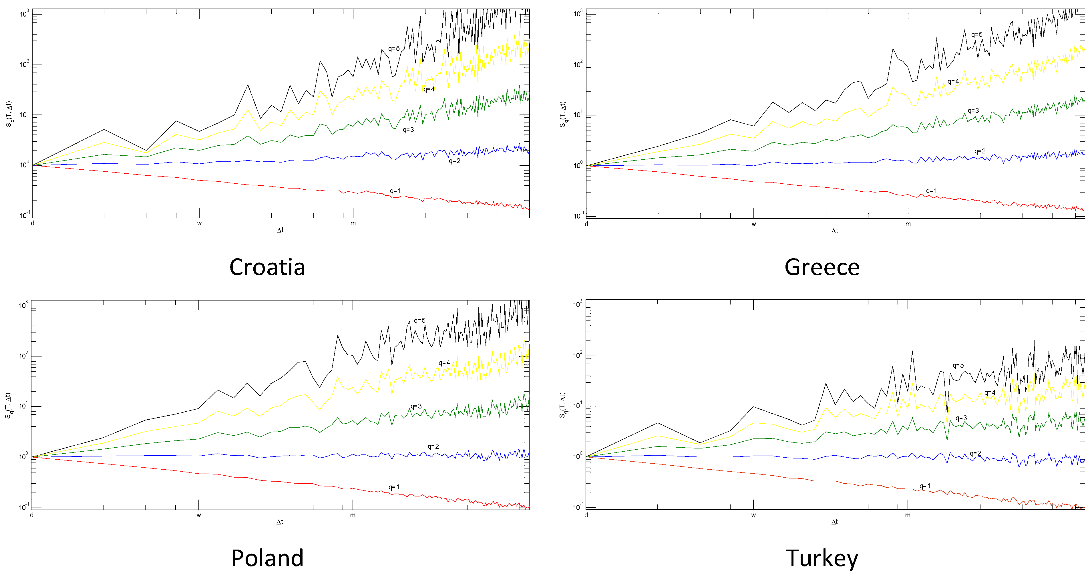
3.1. Multiscaling Property

Before the examination of MMAR, following the definition of Mandelbrot et al. [14], we analyze the multiscaling behavior. As stated before, the scaling property for the self-affine process can be defined as follows:

$$X\left(ct\right)\stackrel{d}{=}{c}^{H}X\left(t\right)$$

(1)

Multifractal theory contains a broader set of conditions:

$$X\left(ct\right)\stackrel{d}{=}M\left(c\right)X\left(t\right)$$

(2)

where $X$ and $M$ are independent random functions. Therefore, multifractality allows greater behavior variety than a self-affine process. The random scaling factor, on the other hand, satisfies the following property: $M\left(ab\right)\stackrel{d}{=}{M}_1\left(a\right)M_2\left(b\right)$, where $M_1$ and $M_2$ are independent copies of $M$, which also satisfies the scaling rule below:

$$\mathbb{E}\left({\left|X\left(t\right)\right|}^q\right)=c\left(q\right)t^{\tau \left(q\right)+1}$$

(3)

where $c\left(q\right)$ and $\tau \left(q\right)$ are the deterministic functions of $q$. This scaling rule is the basic property of the multifractality. $\tau \left(q\right)$ is also stated as a scaling function. A self-affine process with index $H$ is multifractal with the following scaling function: $\tau \left(q\right)=Hq-1$. Because of its linearity, the scaling function is only determined by the slope coefficient and exhibits a uniscaling (unifractal) structure. In spite of that, a concave scaling function exists in a multifractal process.

3.2. The Multifractal Model of Asset Returns

By using the definition of Calvet and Fisher [44], the acquisition process of MMAR can be summarized as follows: the price of an asset $P\left(t\right)$ is in a limited interval $\left[0,T\right]$, and the logarithmic price process is as below:

$$X\left(t\right)\equiv ln P\left(t\right)-\text{ln} P\left(0\right)$$

(4)

By compounding a Brownian motion with the multifractal trading time, we can model the $X\left(t\right)$ process:

Assumption 1. 

$X\left(t\right)$ is a compounding process:

$$X\left(t\right)\equiv B_H\left[\theta \left(t\right)\right]$$

(5)

where $B_H\left(t\right)$ is a fractional Brownian motion and $\theta \left(t\right)$ is stochastic trading time.

Assumption 2. 

Trading time $\theta \left(t\right)$ is the cdf of the multifractal measure $\mu$ defined on interval $\left[0,T\right]$.

Assumption 3. 

$B_H\left(t\right)$ and $\theta \left(t\right)$ processes are independent.

As demonstrated by Fisher et al. [43] when dividing $\left[0,T\right]$ into $N$ intervals of the length $\Delta t$, the partition functions will be as follows:

$$S_q\left(T,\Delta t\right)\equiv {\displaystyle \sum _{i=0}^{N-1}}{\left|X\left(i\Delta t,\Delta t\right)\right|}^q$$

(6)

Despite the fact that there are temporary correlations, in conjunction with the stable increments property of a multifractal process, addends are distributed identically. When the q-th moments exist, if the $X\left(t\right)$ is multifractal, the scaling law satisfies the condition below:

$$\text{log}\mathbb{E}\left[S_q\left(T,\Delta t\right)\right]=\tau \left(q\right)\text{log}\left(\Delta t\right)+c\left(q\right)\text{log}T$$

(7)

At a later stage, graphs of the log $S_q\left(\Delta t\right)$ versus $\text{log}\left(\Delta t\right)$ are plotted for different $q$ and $\Delta t$. The slope of the graph with related $q$ orders is used to test the applicability of MMAR; in other words, the slope of these lines obtained via the OLS method gives an estimation of the scaling function $\tau \left(q\right)$. The estimated scaling function can be easily converted to the estimated multifractal spectrum. As stated by Calvet and Fisher [44], the first two parameters of four ($H$, $\alpha$, $\lambda$, ${\sigma }^2$), which compose the MMAR, can be obtained using the features of the scaling function. Properties of the scaling function are as below:

$$\tau \left(1/H\right)=0$$

(8)

$$f\left(\alpha \right)=\underset{\mathrm{q}}{\text{inf}}\left[\alpha q-\tau \left(q\right)\right]$$

(9)

The first of these two equations gives the inverse ($1/H$) of the Hurst exponent $H$ of the $X\left(t\right)$ process. As stated by Jamdee and Los [46], the same result can be obtained through the plot of partition function, which is approximately parallel to the horizontal axis at a special $q$ moment. As for the second equation, multifractal spectrum $f\left(\alpha \right)$ is the Legendre transformation of the scaling function $\tau \left(q\right)$, that is the Legendre transformation enables the obtaining of the multifractal spectrum $f\left(\alpha \right)$. As demonstrated by Jamdee and Los [46], the first two parameters of the lognormal distribution are attained through the following equations:

$$\lambda =\frac{{\alpha }_0}{H}$$

(10)

$${\sigma }^2=\frac{2\left(\lambda -1\right)}{\text{log} 2}$$

(11)

Equations (10) and (11) give the mean and variance of the lognormal distribution, respectively. The measure that yields the trading time of MMAR can be attained using this closed form.

3.3. FIGARCH Model and Scaling

The FIGARCH model, which gives the fractional differencing parameter $d$, is a parametric approximation of the long memory issue, unlike Mandelbrot’s $R/S$ analysis, which models the long memory via a non-parametric methodology and defines the memory level with the Hurst exponent $H$. Therefore, the long memory property can be explained by these two methodologies: for a stable Gaussian process ($X_i,i\ge 1$) with mean zero, the autocovariance function is $\gamma \left(k\right)=E{X}_i{X}_{i+H}$, and $\gamma$ has the following property:

$$\gamma \left(k\right)~k^{2H-2} f\left(k\right) as k\to \infty$$

(12)

where $f(.)$ is a slowly changing function. $X_i$ is a white noise process for $H=0.5$, while it has a long memory property for $0.5<H<1$ [19]. Similarly, long memory can be defined with $d$ notation via an autocovariance function, which decays hyperbolically:

$$\gamma \left(k\right)~k^{2d-1} f\left(k\right) as k\to \infty$$

(13)

where $d$ is the long memory parameter, and for $0<d<0.5$, the process has long memory. The relationship between $d$ and $H$ is as follows: $d=H-0.5$ [49]. Following Baillie et al. [32], the FIGARCH ($p,d,q$) model can be defined as follows:

$$\left[1-\mathit{\beta }\left(\mathit{L}\right)\right]{\mathit{\sigma }}_{\mathit{t}}^2=\mathit{\omega }+\left[1-\mathit{\beta }\left(\mathit{L}\right)-\mathit{\varphi }\left(\mathit{L}\right){\left(1-\mathit{L}\right)}^{\mathit{d}}\right]{\mathit{\epsilon }}_{\mathit{t}}^2$$

(14)

where $0<d<1$, L denotes the lag operator and ${\left(1-L\right)}^d$ is the fractional differencing operator. In Equation (14), all roots of $\varphi \left(L\right)$ and [$1-\beta \left(L\right)$] are outside of the unit circle.

4. Empirical Analysis

At this stage of the paper, we analyze the multifractal structure of the Croatian, Greek, Polish and Turkish stock markets via the index series: CROBEX, WIG30, ATHEX and BIST100, respectively. The purpose of the empirical investigation is to compare the performance of the GARCH, EGARCH, FIGARCH, MRS-GARCH and MMAR and to determine which model best fits the data in the modeling of stock market index returns. In similar studies, such as Calvet and Fisher [44], Fillol [45] and Jamdee and Los [46], the authors limited the models to normal distributions and used only the GARCH, FIGARCH and GBM in comparing the performance of models with MMAR. In this study, we added the EGARCH and MRS-GARCH models to enhance the model diversity and also used different types of distributions under the FIGARCH and MRS-GARCH models in order to obtain the most efficient results. Our empirical analysis consists of two parts: in the first section, we conducted the parameter estimations of the GARCH, EGARCH, FIGARCH, MRS-GARCH and MMAR models. All of these models have different features. For instance, while the GARCH models the conditional variance and considers the volatility clusterings, the EGARCH contains the asymmetrical structure of the volatility. The FIGARCH, on the other hand, takes the long memory features of the volatility into account. As for MRS-GARCH, it is superior to the previous uni-regime models when the data have different regime properties due to the fact that it considers the multiple regimes in the data. As stated before, the advantage of the MMAR model is its ability to model the most important stylized facts of the financial time series, such as fat tails, long memory and trading time properties.

Following the estimation of the model parameters, scaling functions of the return series are calculated for different $q$ orders ($q=1,2,3,4,5$). The second section of the empirical analysis is allocated to the simulation studies. In this section, using the parameters obtained via the model estimations, simulated time series will be created, and scaling functions of the new series will be calculated. Here, we seek to determine which simulated model’s scaling function results best match those of the original data. The data range of the study consisted of the period of 4 January 2004–3 July 2014 with a total of 3633 observations. Log-returns used in the study are calculated as follows:

$$R_t=\left[ln \left(\frac{P_t}{P_{t-1}}\right)\right]$$

(15)

The models estimated in the empirical analysis and related software/codes are listed in the

Table 1. Used codes and software.

Models	Model Parameters	Model Simulation
GARCH, EGARCH, FIGARCH	Ox-Metrics	Sheppard [50]
		Matlab MFE Toolbox
MRS-GARCH	Marcucci [51]	Chuffart [52]
	MRS-GARCH MATLAB toolbox	MRS-GARCH toolbox
MMAR	Ihlen [53]	Wengert [54]
	MF-DFA MATLAB toolbox	MMAR MATLAB codes
Partition Function	Martineau [55]	-
	MATLAB codes

below.

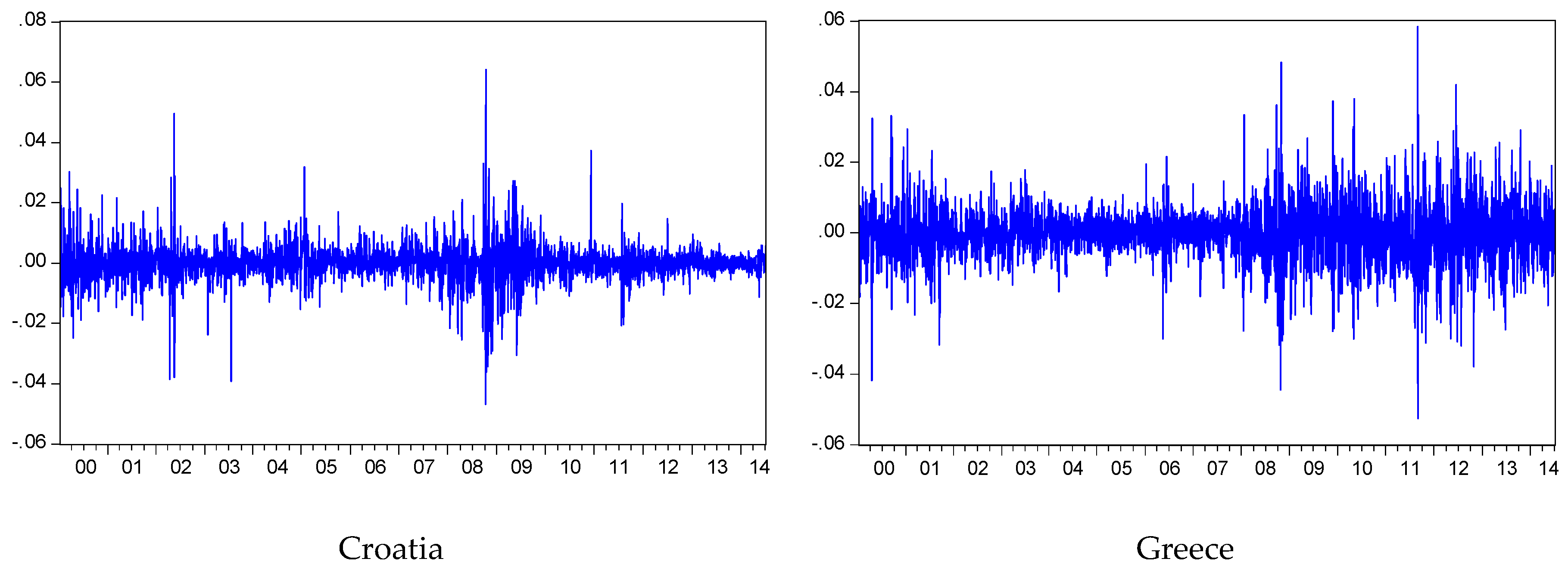
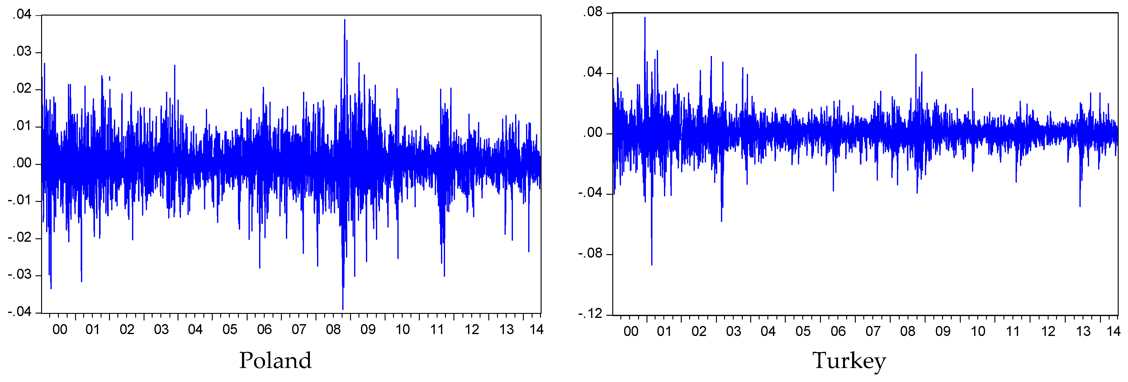
4.1. Descriptive Statistics

Before we evaluate the performance of MMAR and other models, first we determined the descriptive statistics of the series to see the characteristic features of the variables. The result obtained for descriptive statistics are represented in

Table 2. Descriptive statistics of the original series.

Statistics	Croatia	Greece	Poland	Turkey
Mean	0.000104	−0.00018	0.0000423	0.000178
SD	0.00581	0.007811	0.006685	0.009988
Skewness	0.097397	−0.02117	−0.13425	−0.06851
Kurtosis	16.5597	7.639252	5.761347	9.77734
Jarque-Bera	27,838 ***	3258 ***	1165 ***	6956 ***

^*** denotes significance at the 99% confidence level.

below.

As can be seen from the results, all mean values are close to zero with only Greek stock market returns having a negative mean value. According to the standard deviation statistic, which is the most primitive way to measure risk, the highest volatility in the return series belongs to the Turkish stock market, with the Greek stock market second. In addition to the mean and standard deviation, we have seen that skewness and kurtosis values present deviations from the normal distribution of asset returns. Except for Croatia, the series demonstrates a negative asymmetry by the left tail of the distribution being longer than the right tail. The Jarque-Bera test statistic also displays that all of the return series are quite far away from the normal distribution. Besides the statistical feature of the return series, we have also represented the chart of all of them in Figure 1 below to see the way they follow in the period of study.

Since our study is based on the multifractality and long memory, as a diagnosis, we first conducted monofractal analysis to see the memory properties of the series through two well-known Hurst exponent methods: the Detrended Fluctuation Analysis (DFA) and the aggregated variance method. Results are can be seen in

Table 3. Monofractal H statistics for the original series.

Methods	Croatia	Greece	Poland	Turkey
Detrended Fluctuation Analysis	0.5397 ***	0.5166 ***	0.4805 ***	0.4832 ***
	(−0.0199)	(−0.0152)	(−0.0201)	(−0.0094)
Aggregated Variance	0.6294 ***	0.5878 ***	0.5435 ***	0.5084 ***
	(0.0297)	(0.0294)	(0.0513)	(0.0444)

*** denotes significance at the 99% confidence level.

below. Kim et al. [56] and Günay [57] showed the performance of these two models against the alternatives in the estimation of the monofractal Hurst exponent. The most important feature of the DFA is providing consistent results even in non-stationary series.

According to the results obtained for DFA, the monofractal Hurst exponent H is around the threshold value of 0.5. While it is slightly higher than 0.5 for Croatia and Greece, in the other two variables, Poland and Turkey, it is lightly less than 0.5. In addition, the results of the aggregated variance test are surprisingly close to the findings of MMAR analysis. In both models, the highest H values are obtained for Croatia, Greece, Poland and Turkey, respectively. The aggregated variance analysis Hurst exponent value for Turkey is equal to 0.5, which is the reference number of the market efficiency. This result will be also obtained under MMAR analysis later on.

4.2. Parameter Estimations

As previously stated, the first section of the empirical analysis consists of the parameter estimations. In accordance with this purpose, first, we estimated the GARCH (1.1) model. As seen from

Table 4. GARCH (1.1) parameters of the log returns of the original series.

Countries	$\omega$	$\alpha$	$\beta$
Croatia	0.292444	0.085159 **	0.911678 **
	(0.17881)	(0.026237)	(0.027485)
Greece	0.516918 *	0.090307 **	0.905742 **
	(0.23256)	(0.01795)	(0.019015)
Poland	0.380276 **	0.061464 **	0.930645 **
	(0.12473)	(0.0082957)	(0.0089465)
Turkey	0.013341 *	0.103096 **	0.886660 **
	(0.0053819)	(0.021269)	(0.023662)

* and ** indicate the 95% and 99% confidence level, respectively.

, alpha and beta values of the GARCH (1.1), the sum of these statistics is close to one. According to Engle and Bollerslev [58], this situation shows persistence in volatility in which unconditional variance approaches zero very slowly, indicating the long memory property in the variance of the return series.

In order to consider the asymmetry property of volatility, as a second model, in

Table 5. EGARCH (1.1) parameters of the log returns of the original series.

Countries	$\omega$	$\alpha$	$\gamma$	$\beta$
Croatia	−0.305014 **	0.197241 **	−0.008751 *	0.984521 **
	(0.015919)	(0.007293)	(0.004147)	(0.001323)
Greece	−0.273209 **	0.163630 **	−0.043302 **	0.984898 **
	(0.021986)	(0.009035)	(0.004873)	(0.001950)
Poland	−0.227455 **	0.125215 **	−0.036094 **	0.987054 **
	(0.025928)	(0.009624)	(0.005910)	(0.002256)
Turkey	−0.376273 **	0.208343 **	−0.052680 **	0.977284 **
	(0.027994)	(0.010824)	(0.006009)	(0.002656)

* and ** indicate the 95% and 99% confidence level, respectively.

below we estimated EGARCH (1.1). EGARCH models the asymmetrical effects produced by past shocks in the volatility. Therefore, changes occurring in the volatility against good and bad news are incorporated by the model. Asymmetrical effects are caught by the parameter $\gamma$. As the results exhibit, the asymmetry parameter $\gamma$ in EGARCH (1.1) is statistically significant at a 95% confidence level for all stock markets. This finding demonstrates the existence of a leverage effect, that is negative return shocks create higher volatility than positive returns. According to the results in Table 5, the largest γ values belong to Turkey, Greece, Poland and Croatia, respectively. As a result, we can say that the highest effect in volatility created by negative return shocks occurs in the Turkish stock market.

As the results of the GARCH (1.1) model indicate, there is a persistent or long range dependence in volatility. At this stage, we continue the analysis with the FIGARCH, which takes the long memory property in volatility into account. As seen in

Table 6. FIGARCH (1.1) parameters of the log returns of the original series.

Countries	$\omega$	$d$	$\alpha$	$\beta$	Asymmetry	Tail	GED
Croatia	0.5652	0.4498 **	0.4124 **	0.6391 **	-	-	1.0075
	(0.3075)	(0.0712)	(0.1262)	(0.1314)			(0.0441)
Greece	2.5724 **	0.3566 **	0.1015	0.3849 **	-	-	1.2322
	(0.7623)	(0.0429)	(0.0733)	(0.0891)			(0.0513)
Poland	0.5307 *	0.5753 **	0.2108 **	0.7476 **	-	-	1.2948 **
	(0.2361)	(0.1134)	(0.0488)	(0.0756)			(0.0489)
Turkey	3.6399 **	0.3523 **	0.1235	0.3802 **	−0.0617 **	7.7344 **	-
	(1.3372)	(0.0426)	(0.0993)	(0.1140)	(0.0227)	(0.9032)

* and ** indicate the 95% and 99% confidence level, respectively. GED: Generalized Error Distribution.s

, Parameters of the FIGARCH model were estimated under alternative unconditional distributions, such as normal, Student t, skewed Student t and the Generalized Error Distribution (GED), and decisions were made through the best fitting distribution type. In determining the best distribution type, we considered the Akaike Information Criterion (AIC), Schwartz Information Criterion (SIC) and the log-likelihood statistics of the models. According to the results, GED outperforms the alternative distributions for the index returns of the Croatian, Greek and Polish stock markets. On the other hand, the skewed Student t distribution is the best fitting distribution for the Turkish stock market index returns. Results demonstrate that both asymmetry and tail statistics concerning the Student t distribution are statistically significant. Likewise, the GED distribution test statistic is significant for the FIGARCH model of three countries. The fractional differencing parameter $d$, which tests the long memory property of volatility, is statistically significant at a 95% confidence level for all countries. The parameter in the range of $0<d<0.5$ is evidence of long memory in volatility. Accordingly, except for Poland, all countries’ stock index returns have long memory features. As for Poland, it has a $d$ value in the range of $0.5<d<1$, meaning that it has non-stationary and mean-reverting long memory properties, that is even shocks long passed may affect today’s return.

Parameter estimations of the MRS-GARCH model are exhibited in

Table 7. MRS-GARCH parameters of the log returns of the original series.

Parameters	Croatia	Greece	Poland	Turkey
${\gamma }_L$	0.4705	0.0554	0.0371	−1.3797
	(0.0619)	(0.0234)	(0.0201)	(0.5813)
${\gamma }_H$	0.0000	−0.0425	−1.9493	0.1519
	(0.0082)	(0.0408)	(0.4761)	(0.0294)
${\omega }_L$	0.7287	0.0729	0.0338	0.9673
	(0.4098)	(0.0247)	(0.0119)	(0.4796)
${\omega }_H$	0.0201	0.4484	0.0758	0.0633
	(0.0061)	(0.1344)	(0.9568)	(0.0213)
${\alpha }_L$	0.2965	0.0742	0.0458	0.0470
	(0.1782)	(0.0187)	(0.0107)	(0.0394)
${\alpha }_H$	0.0981	0.1037	0.0320	0.0677
	(0.0151)	(0.0225)	(0.1764)	(0.0118)
${\beta }_L$	0.1757	0.8627	0.9177	0.9497
	(0.3783)	(0.0326)	(0.0114)	(0.0735)
${\beta }_H$	0.8868	0.8002	0.9537	0.8861
	(0.0139)	(0.0419)	(0.3109)	(0.0122)
$p$	0.9341	0.9991	0.9916	0.7518
	(0.0247)	(0.0007)	(0.0034)	(0.0904)
$q$	0.9922	0.9995	0.6206	0.9839
	(0.0034)	(0.0006)	(0.1313)	(0.0069)

below. Similar to the FIGARCH model, in the MRS-GARCH model, we used different types of unconditional distributions, and the most successful results were obtained through the GED for all of the index returns.

Results in Table 7 confirm the existence of two different regimes in the return volatility of every country. Parameter ${\omega }_i$, which displays the long-term behavior of the volatility, acts quite differently for every country under two regimes. As for $\alpha$ and $\beta$, they represent the short-term behavior of the volatility. Accordingly, there is a high persistence in the second regime for the returns of Croatia, whereas there is no persistence in the first regime. Likewise, the second regime in the Polish returns has a higher persistence than the first. On the other hand, Greece and Turkey’s first regime’s volatility is stronger than the second’s. It is noteworthy that all three countries’ volatility persistence is distinctly high for both regimes. While transition probabilities are statistically significant for all countries, the related statistic is relatively far from unity for Poland and Turkey.

In order to determine whether the return series are monofractal or multifractal, we determined the scaling function plot of all four indexes versus different $q$ orders between −5 and 5. As stated by Mandelbrot et al. [14] the scaling function has a linear shape in monofractal time series, while it is nonlinear for the multifractal time series. According to the results of Figure 2, scaling functions of all index returns have a nonlinear and concave structure. In addition, the highest degree of non-linearity is seen in the returns of Croatia and Turkey. Therefore, we can say that the highest multifractality features belong to the returns of the Croatian and Turkish stock markets.

Figure 3 displays the partition functions of Croatian, Greek, Polish and Turkish stock markets, respectively. Likewise, for the definition of MMAR established in Section 3, the partition function is obtained by the following process using the interpretation of Calvet and Fisher [44]: logarithmic form of the price series $P\left(t\right)$ in time interval $\left[0,T\right]$ is $X\left(t\right)\equiv lnP\left(t\right)-lnP\left(0\right)$. By partitioning the $\left[0,T\right]$ into $N$ integer intervals of a length of $\Delta t$, partitioning functions can be defined as follows:

$$S_q\left(T,\Delta t\right)\equiv {\displaystyle \sum _{i=0}^{N-1}}{\left|X\left(i\Delta t+\Delta t\right)-X\left(i\Delta t\right)\right|}^q$$

(16)

In cases where any function has the scaling property, the logarithmic graph of the partition function versus time increments should be approximately linear [46]. In addition, the $q$ value, which is parallel to the horizontal axis, presents the related Hurst exponent $H$ value. On the other hand, in order to calculate the exact value of the Hurst exponent $H$, we used the following relationship $\tau \left(q=1/H\right)=0$, given in Equation (8).

According to the obtained $q$ values in

Table 8. Estimated $q$ values of the log returns of the original series.

	Croatia	Greece	Poland	Turkey
$q$	1.6331	1.8368	1.8595	2.0000

for Croatia, Greece, Poland and Turkey, we see that the partition functions have zero slope and a slight persistence with the following values. Approximate results can be seen from Figure 3. Accordingly, it is clear that the partition functions of all indexes’ returns are roughly parallel to the horizontal axis for $q=2$.

Table 9. MMAR parameters of the original series.

Countries	H	${\alpha }_0$	$\lambda$	${\sigma }^2$
Croatia	0.6123	0.6392	1.0439	0.1268
Greece	0.5444	0.5522	1.0143	0.0411
Poland	0.5378	0.5524	1.0272	0.0783
Turkey	0.5000	0.5455	1.0910	0.2597

below presents the results of the parameters required to construct the MMAR. As stated by Jamdee and Los [46], in order to model the conditional variance property of the time series and to take true scaling features into account, the MMAR requires four parameters: the Hurst exponent $H$ value of the return series, the most probable Hurst exponent value of the trading time (${\alpha }_0$) and the first and second moments of the lognormal distributions of multiplicative probability measures $(\lambda$ and ${\sigma }^2)$. It is worth noting that only one Hurst exponent, that is a monofractal Hurst exponent, is calculated in the construction of MMAR. After obtaining the $H$ and ${\alpha }_0$ parameters, we calculated the first and second moments ($\lambda$ and ${\sigma }^2$) of the lognormally-distributed multinomial measures.

These results demonstrate that the highest persistence in the volatility of the index returns occurs in Croatia concerning $H$ values. On the other hand, the $H$ value of Turkey is 0.50, which is the Hurst exponent value of geometric Brownian motion. This result indicates that Turkish stock index returns perform a random walk behavior as assumed by the efficient market hypothesis and do not possess long memory features. In other words, Turkish stock market returns demonstrate a fully-stochastic random behavior, and fluctuations follow white noise. Similar to the findings of Jamdee and Los [46], another interesting result is that the first moment of the lognormal return distribution is larger than one for all countries. In addition, the highest $\lambda$ statistic is seen in the return distribution of Turkey, which means that there is an indistinct relationship between the persistency level of the market and the persistency level of information process in the Turkish stock market. Similarly, it is clear that the variance level of Turkey ${\sigma }^2$ is also higher than those of other countries. This demonstrates that the Turkish stock market is affected by a wider variety of news events.

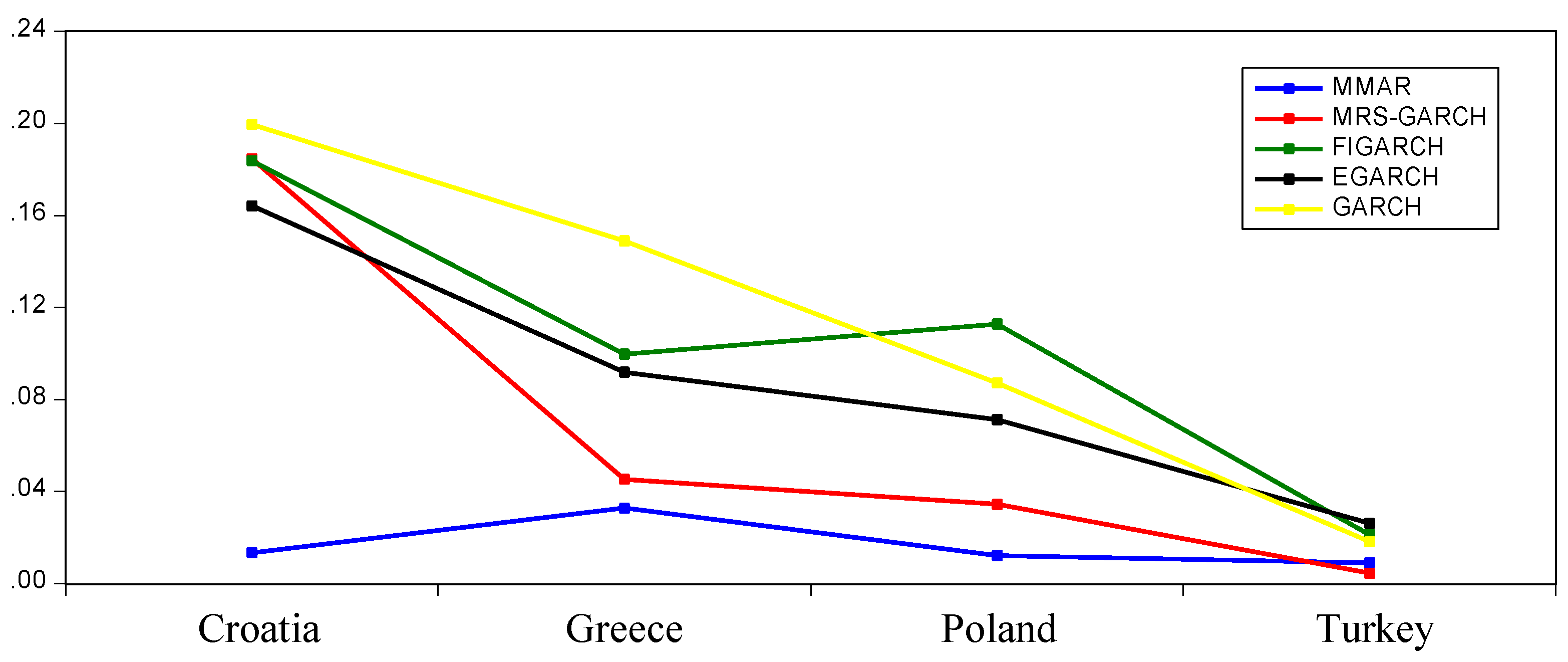
4.3. Simulations and Construction of the Models

Using the acquired parameters of the MMAR, GARCH, EGARCH, FIGARCH and MRS-GARCH models, at this stage of the study, we produce 1000 different simulated time series for every model with the Monte Carlo simulation method. The reason for using the Monte Carlo simulations is to assess the replicability of the simulated time series in order to analyze the performance of the alternative models. The purpose here is to compare scaling function values obtained using the original return series and the simulated return series. The scaling function values of the original and simulated time series for different $q$ orders ($q=1,2,3,4,5$) are presented in

Table 10. Scaling function values of the empirical and simulated series.

	$\raisebox{1ex}{$\mathbf{q}$}\!\left/ \!\raisebox{-1ex}{$\tau $}\right.$	${\widehat{\tau }}_{empirical}$	MMAR $\overline{\tau }$	GARCH (1.1) $\overline{\tau }$	EGARCH (1.1) $\overline{\tau }$	FIGARCH (1.1) $\overline{\tau }$	MRS-GARCH $\overline{\tau }$
			Simulation Results
Croatia	1	−0.39	−0.38	−0.48	−0.49	−0.48	−0.53
	2	0.21	0.20	−0.01	−0.01	−0.01	−0.09
	3	0.76	0.76	0.40	0.42	0.41	0.32
	4	1.27	1.28	0.76	0.81	0.79	0.71
	5	1.74	1.77	1.09	1.18	1.13	1.08
Greece	1	−0.45	−0.45	−0.48	−0.49	−0.49	−0.46
	2	0.09	0.08	−0.01	−0.01	−0.01	0.07
	3	0.59	0.59	0.39	0.43	0.43	0.59
	4	1.05	1.08	0.75	0.83	0.82	1.09
	5	1.47	1.54	1.07	1.20	1.18	1.56
Poland	1	−0.46	−0.45	−0.49	−0.50	−0.49	−0.50
	2	0.07	0.07	−0.01	−0.02	-0.01	−0.01
	3	0.57	0.57	0.44	0.44	0.42	0.46
	4	1.04	1.05	0.85	0.86	0.81	0.92
	5	1.48	1.51	1.23	1.26	1.17	1.36
Turkey	1	−0.47	−0.47	−0.48	−0.49	−0.49	−0.48
	2	0.00	0.00	−0.01	−0.02	−0.02	−0.01
	3	0.42	0.42	0.40	0.42	0.42	0.41
	4	0.80	0.81	0.76	0.82	0.81	0.78
	5	1.14	1.16	1.09	1.18	1.17	1.13

below. Since the simulation model that has the closest scaling function values to the original series will be accepted as the best replica model, we will consider it as the best alternative model that contains the same stylized facts in the original series. It is also worth noting that unlike the original return series, the scaling function values of the simulated models were attained through the mean values of $\tau$ of the 1000 simulated time series for all countries and models. As for the scaling function values of empirical data, they were obtained by means of the slopes of the partition functions.

The results of Table 10 demonstrate that $q=1$ values start as negative for all countries’ index returns, and ultimately, $q=5$ ends in a value of around 1.5. In order to carry out a more thorough evaluation about the results of Table 10, we present the standard deviations of the differences between the original series’ scaling function values and those of the simulated series in

Table 11. Standard deviation of the scaling function values from ${\widehat{\tau }}_{empirical}$.

Countries	MMAR $\overline{\tau }$	GARCH (1.1) $\overline{\tau }$	EGARCH (1.1) $\overline{\tau }$	FIGARCH (1.1) $\overline{\tau }$	MRS-GARCH $\overline{\tau }$
Croatia	0.0133	0.1995	0.1641	0.1838	0.1846
Greece	0.0327	0.1489	0.0918	0.0996	0.0453
Poland	0.0122	0.0871	0.0712	0.1127	0.0344
Turkey	0.0089	0.0182	0.0261	0.0212	0.0045

. It is clear that larger deviation figures mean inferior performance for the related models.

When we look at the findings of the simulated Croatia, Greece and Poland series, we see that among the simulated time series, the results that best match the original series are provided by the MMAR. However, regarding Turkey, the situation differs slightly from the others. Despite the fact that the MMAR and MRS-GARCH results are approximately equal in the Turkish stock market, the MRS-GARCH model slightly outperforms the MMAR with a difference of 0.0044. On the other hand, although the GARCH model catches the time-varying volatility, skewness and kurtosis features that arise in the financial time series, it does not properly identify the empirical index return processes. Because it also considers the different reaction property of variance against good and bad news, we can see relatively better results in the EGARCH model when compared to GARCH. Besides, the performance of the FIGARCH model, which takes long memory into account in analogy to MMAR, fell short of our expectations, as well. In spite of that, the MRS-GARCH model produced the second most successful results after MMAR. Not only does the MRS-GARCH model best fit the data of Turkey, it also displays the second best performance for Greek and Polish index returns. If we pay attention, it is clear that there is an obvious relationship between the Hurst exponent value and the performance of the MRS-GARCH model. While the MRS-GARCH model performed poorly for Croatian returns with the highest Hurst exponent value, the same model exhibits moderately successful results for Greece and Poland, which have comparatively lower Hurst exponent values. Additionally, for the Turkish stock returns, which have an $H$ value of 0.5, indicating the absence of long memory or the existence of the random walk, the MRS-GARCH is slightly more successful than the MMAR. Since there are no long memory features in the return diffusion process of the Turkish stock market, the performances of the MMAR and MRS-GARCH models appear quite close, the reasons for which are worthy of examination in another study or dissertation. As a general assessment, we can say that the MMAR displays the best replica performance against the alternative models in reflecting the stylized facts of original return series. Upon deep inspection, we see that MMAR preserves the scaling properties of different stock index returns especially for the first three moments, while fourth and fifth moments are slightly higher than the empirical results.

Information concerning previous results can also be viewed in Figure 4. Loosely speaking, the lowest deviations from the original series were obtained with the MMAR. The second best model is the MRS-GARCH. Accordingly, we can say that MMAR is superior to the GARCH, EGARCH and FIGARCH models in the modeling of the time-scaling properties of the stock index returns. The results obtained from the empirical section of this study are generally consistent with the findings of Calvet and Fisher [44], Fillol [45], Jamdee and Los [46]. Distinct from these studies, the most interesting result in our analysis concerns MRS-GARCH’s performance. We saw that when the persistency decreases or in the absence of long memory features, MRS-GARCH displays a high performance similar to MMAR.

5. Conclusions

In this study, the performance of the multifractal model of asset returns was analyzed in comparison to other popular models, such as GARCH, EGARCH, FIGARCH and MRS-GARCH during the period of 4 January 2004–3 July 2014 for the stock index returns of Croatia, Greece, Poland and Turkey. According to the parameter estimations conducted in the first section of the empirical analysis, the sum of the mean and variance parameters in the GARCH model have values very close to unity as a result of high persistency. As for the other models, EGARCH exhibited asymmetrical effects; FIGARCH demonstrated long memory; while MRS-GARCH showed the existence of different regimes in the volatility. According to the parameter estimations of MMAR, the highest persistence in stock index returns was seen in the Croatian, Greek, Polish and Turkish stock markets respectively. The most interesting result concerning Hurst exponent $H$ was obtained for Turkey. As distinct from the other countries’ results, the Turkish stock market had an $H$ value equal to 0.5, indicating the existence of the random walk in the log returns. In the second section of empirical analysis, we simulated 1000 paths for each model through Monte Carlo simulations using the previous parameters obtained in the first section. Afterwards, scaling function values were calculated for both original and simulated time series in different $q$ orders ($q=1,2,3,4,5$). When we compare the results of the original and simulated time series, the best fitting replication of the original series’ time-varying variance process was exhibited by the MMAR. Other interesting results were the increasing performance of MRS-GARCH for the lower values of $H$ and its matching with the performance of MMAR for the random walk process. Hence, for Turkey, which has an $H$ value equal of 0.5, the performance of the MRS-GARCH model is more successful than MMAR with a difference of 0.0044.

References

1. E. Fama. “Random Walks in Stock Market Prices.” Financ. Anal. J. 21 (1965): 55–59. [Google Scholar] [CrossRef]
2. E. Fama. “Efficient Capital Markets: A Review of Theory and Empirical Work.” J. Financ. 25 (1970): 383–417. [Google Scholar] [CrossRef]
3. B.B. Mandelbrot. “The Pareto-Lévy law and the distribution of income.” Int. Econ. Rev. 1 (1960): 79–106. [Google Scholar] [CrossRef]
4. B.B. Mandelbrot. “The variation of certain speculative prices.” J. Bus. 36 (1963): 392–417. [Google Scholar] [CrossRef]
5. B.B. Mandelbrot, and J.R. Wallis. “Some Long-Run Properties of Geophysical Records.” Water Resour. Res. 5 (1969): 321–340. [Google Scholar] [CrossRef]
6. H.E. Hurst. “Long-term storage capacity of reservoirs.” Trans. Am. Soc. Civ. Eng. 116 (1951): 770–808. [Google Scholar]
7. M.S. Taqqu. “Benoit Mandelbrot and Fractional Brownian Motion.” Stat. Sci. 28 (2013): 131–134. [Google Scholar] [CrossRef]
8. E.E. Peters. Fractal Market Analysis: Applying Chaos Theory to Investment and Economics. New York, NY, USA: John Wiley and Sons, 1994. [Google Scholar]
9. J. Beran, Y. Feng, S. Ghosh, and R. Kulik. Long-Memory Processes: Probabilistic Properties and Statistical Methods. New York, NY, USA: Springer, 2013. [Google Scholar]
10. A.B. Schmidt. Financial Markets and Trading: An Introduction to Market Microstructure and Trading Strategies. New York, NY, USA: John Wiley & Sons, 2011. [Google Scholar]
11. J. Goddard, and E. Onali. “Self-affinity in financial asset returns.” Int. Rev. Financ. Anal. 24 (2012): 1–11. [Google Scholar] [CrossRef]
12. R. Engle. “Autorregressive Conditional Heteroskedasticity with Estimates of United Kingdom Inflation.” Econometrica 50 (1982): 987–1008. [Google Scholar] [CrossRef]
13. T. Bollerslev. “Generalized Autorregressive Conditional Heteroskedasticity.” J. Econom. 31 (1986): 307–327. [Google Scholar] [CrossRef]
14. B.B. Mandelbrot, A. Fisher, and L. Calvet. “A multifractal model of asset returns.” Cowles Foundation Discussion Paper No. 1164; New Haven, CT, USA: Yale University, 1997, pp. 1–33. [Google Scholar]
15. F.C. Drost, and J.C. Werker. “Closing the GARCH gap: Continuous GARCH modelling.” J. Econom. 74 (1996): 31–57. [Google Scholar] [CrossRef]
16. B.B. Mandelbrot. “Statistical Methodology for Nonperiodic Cycles from Covariance to R/S Analysis.” In Annals of Economic and Social Measurement. Cambridge, MA, USA: National Bureau of Economic Research, 1972, Volume 1, pp. 259–290. [Google Scholar]
17. A.W. Lo. “Long-term memory in stock market prices.” Econometrica 59 (1991): 1279–1313. [Google Scholar] [CrossRef]
18. C.K. Peng, S.V. Buldyrev, S. Havlin, M. Simons, H.E. Stanley, and A.L. Goldberger. “Mosaic organization of DNA nucleotides.” Phys. Rev. E 49 (1994): 1685–1689. [Google Scholar] [CrossRef]
19. M. Taqqu, V. Teverovsky, and W. Willinger. “Estimators for long-range dependence: An empirical study.” Fractals 3 (1995): 785–798. [Google Scholar] [CrossRef]
20. M.S. Taqqu, and V. Teverovsky. “Robustness of Whittle type estimators for time series with long-range dependence.” Stoch. Models 13 (1997): 723–757. [Google Scholar] [CrossRef]
21. P. Abry, and D. Veitch. “Wavelet analysis of long-range-dependent traffic.” IEEE Trans. Inf. Theory 44 (1998): 2–15. [Google Scholar] [CrossRef]
22. C.W.J. Granger, and R. Joyeux. “An introduction to loag memory time series models and fractional differencing.” J. Time Ser. Anal. 1 (1980): 5–39. [Google Scholar]
23. J.R.M. Hosking. “Fractional differencing.” Biometrika 68 (1981): 165–176. [Google Scholar] [CrossRef]
24. J. Geweke, and S. Porter-Hudak. “The estimation and Appication of Long Memory Time Series Models.” J. Time Seri. Anal. 4 (1983): 221–238. [Google Scholar] [CrossRef]
25. P.M. Robinson. “Log-periodogram regression of time series with long range dependence.” Ann. Stat. 23 (1995): 1048–1072. [Google Scholar] [CrossRef]
26. P.C.B. Phillips. “Discrete Fourier Transforms of Fractional Processes; 1999.” New Haven, CT, USA; Unpublished Working Paper No. 1243. : Cowles Foundation for Research in Economics; Yale University. Available online: http://cowles.yale.edu/sites/default/files/files/pub/d12/d1243.pdf (accessed on 23 July 2014).
27. P.C.B. Phillips. “Unit Root Log Periodogram Regression; 1999.” Cowles Foundation for Research in Economics; Yale University; Unpublished Working Paper No. 1244. Available online: http://cowles.yale.edu/sites/default/files/files/pub/d12/d1244.pdf (accessed on 23 July 2014).
28. A. Smith. “Level Shifts and the Illusion of Long Memory in Economic Time Series.” J. Bus. Econ. Stat. 23 (2005): 321–335. [Google Scholar] [CrossRef]
29. K. Shimotsu, and P.C.B. Phillips. “Exact Local Whittle estimation of fractional integration.” Ann. Stat. 33 (2005): 1890–1933. [Google Scholar] [CrossRef]
30. K.M. Abadir, W. Distaso, and L. Giraitis. “Non-stationarity extended Local Whittle estimation.” J. Econom. 141 (2007): 1353–1384. [Google Scholar] [CrossRef]
31. K. Shimotsu. Simple (but Effective) Tests of Long Memory versus Structural Breaks. Queen’s Economics Department Working Paper No. 1101; Kingston, ON, Canada: Queen’s University, 2006. [Google Scholar]
32. R.T. Baillie, T. Bollerslev, and H.O. Mikkelsen. “Fractionally integrated Generalized Autoregressive Conditional Heteroscedasticity.” J. Econom. 74 (1996): 3–30. [Google Scholar] [CrossRef]
33. T. Bollerslev, and H.O. Mikkelsen. “Modeling and pricing long memory in stock market volatility.” J. Econom. 73 (1996): 151–184. [Google Scholar] [CrossRef]
34. B.J. Christensen, M.Ø. Nielsen, and J. Zhu. “Long memory in stock market volatility and the volatility-in-mean effect: The FIEGARCH-M Model.” J. Empir. Financ. 17 (2010): 460–470. [Google Scholar] [CrossRef]
35. R. Kilic. “Long memory and nonlinearity in conditional variances: A smooth transition FIGARCH model.” J. Empir. Financ. 18 (2011): 368–378. [Google Scholar] [CrossRef]
36. J. Davidson, and P. Sibbertsen. “Generating schemes for long memory processes: Regimes, aggregation and linearity.” J. Econom. 128 (2005): 253–282. [Google Scholar] [CrossRef] [Green Version]
37. T. Andersen, and T. Bollerslev. “Heterogeneous information arrivals and return volatility dynamics: Uncovering the long-run in high frequency returns.” J. Finance 52 (1997): 975–1005. [Google Scholar] [CrossRef]
38. P. Zaffaroni. “Aggregation and memory of models of changing volatility.” J. Econom. 136 (2007): 237–249. [Google Scholar] [CrossRef] [Green Version]
39. T. Mikosch, and C. Starica. “Change of Structure in Financial Time Series, Long Range Dependence and the GARCH Model.” Available online: http://citeseerx.ist.psu.edu/viewdoc/versions?doi=10.1.1.56.5517 (accessed on 5 September 2014).
40. F.X. Diebold, and A. Inoue. “Long Memory and Regime Switching.” J. Econom. 105 (2001): 131–159. [Google Scholar] [CrossRef]
41. M. Balcilar. “Long Memory and Structural Breaks in Turkish Inflation Rates.” In Proceedings of the National Econometrics and Statistics Symposium VI, Gazi University, Ankara, Turkey, May 2003; pp. 1–13.
42. R.T. Baillie, and C. Morana. “Modelling long memory and structural breaks in conditional variances: An adaptive FIGARCH approach.” J. Econ. Dyn. Control 33 (2009): 1577–1592. [Google Scholar] [CrossRef]
43. A. Fisher, L. Calvet, and B.B. Mandelbrot. “Multifractality of Deutschemark/US Dollar Exchange Rates.” Cowles Foundation Discussion Paper No.1165; New Haven, CT, USA: Yale University, 1997, pp. 1–77. [Google Scholar]
44. L. Calvet, and A. Fisher. “Multifractality in Asset Returns: Theory and Evidence.” Rev. Econ. Stat. 84 (2002): 381–406. [Google Scholar] [CrossRef]
45. J. Fillol. “Multifractality: Theory and Evidence an Application to the French Stock Market.” Econ. Bull. 3 (2003): 1–12. [Google Scholar]
46. S. Jamdee, and C.A. Los. “Multifractal Modeling of the US Treasury Term Structure and Fed Funds Rate.” 2005. Available online: http://econpapers.repec.org/paper/wpawuwpfi/0502021.htm (accessed on 5 September 2014).
47. S. Jamdee, and C.A. Los. “Multifractal Modeling of the Japanese Treasury Term Structure.” In Japanese Fixed Income Markets: Money, Bond and Interest Rate Derivatives. Edited by J.A. Batten, T.A. Fetherston and P.G. Szilagyi. Amsterdam, The Netherlands: Elsevier Science, 2006, Chapter 12; pp. 285–320. [Google Scholar]
48. J.A. Batten, H. Kinateder, and N. Wagner. “Multifractality and value-at-risk forecasting of exchange rates.” Phys. A Stat. Mech. Appl. 401 (2014): 71–81. [Google Scholar] [CrossRef]
49. W. Palma. Long-Memory Time Series: Theory and Methods. Hoboken, NJ, USA: John Wiley & Sons, 2007. [Google Scholar]
50. K. Sheppard. “MFE MATLAB Function Reference Financial Econometrics.” 2009. Available online: www.kevinsheppard.com/images/9/95/MFE_Toolbox_Documentation.pdf (accessed on 7 August 2014).
51. J. Marcucci. “Forecasting stock market volatility with regime switching GARCH models.” Stud. Nonlinear Dyn. Econom. 9 (2005): 1–53. [Google Scholar] [CrossRef]
52. T. Chuffart. “Readme RSGARCH Toolbox.” Available online: www.thomaschuffart.fr/?page_id=12 (accessed on 13 August 2014).
53. E.A.F. Ihlen. “Introduction to multifractal detrended fluctuation analysis in Matlab.” Front. Physiol. 3 (2012): 1–18. [Google Scholar] [CrossRef] [PubMed]
54. C. Wengert. “Multifractal Model of Asset Returns (MMAR).” Available online: http://www.mathworks.com/matlabcentral/fileexchange/29686-multifractal-model-of-asset-returns--mmar- (accessed on 2 September 2014).
55. C. Martineau. “Partition Function for Scaling Moment.” Available online: www.charlesmartineau.com/?page_id=1196 (accessed on 13 August 2014).
56. B.S. Kim, H.S. Kim, and S.H. Min. “Hurst’s Memory for Chaotic, Tree Ring, and SOI Series.” Appl. Math. 5 (2013): 175–195. [Google Scholar] [CrossRef]
57. S. Günay. “Are the Scaling Properties of Bull and Bear Markets Identical? Evidence from Oil and Gold Markets.” Int. J. Financ. Stud. 2 (2014): 315–334. [Google Scholar] [CrossRef]
58. R.F. Engle, and T. Bollerslev. “Modelling the Persistence of Conditional Variances.” Econom. Rev. 5 (1986): 1–50. [Google Scholar] [CrossRef]
Figure 1. Index returns of Croatia, Greece, Poland and Turkey (4 January 2004–3 July 2014).
Ijfs 04 00011 g001aIjfs 04 00011 g001b
Figure 2. Classical multifractal scaling exponent τ (q) versus q.
Ijfs 04 00011 g002
Figure 3. Partition functions of the log returns of the original series.
Ijfs 04 00011 g003
Figure 4. Path of the standard deviation of scaling function values.
Ijfs 04 00011 g004