Opportunistic In-Flight INS Alignment Using LEO Satellites and a Rotatory IMU Platform

Abstract

With the emergence of numerous low Earth orbit (LEO) satellite constellations such as Iridium-Next, Globalstar, Orbcomm, Starlink, and OneWeb, the idea of considering their downlink signals as a source of pseudorange and pseudorange rate measurements has become incredibly attractive to the community. LEO satellites could be a reliable alternative for environments or situations in which the global navigation satellite system (GNSS) is blocked or inaccessible. In this article, we present a novel in-flight alignment method for a strapdown inertial navigation system (SINS) using Doppler shift measurements obtained from single or multi-constellation LEO satellites and a rotation technique applied on the inertial measurement unit (IMU). Firstly, a regular Doppler positioning algorithm based on the extended Kalman filter (EKF) calculates states of the receiver. This system is considered as a slave block. In parallel, a master INS estimates the position, velocity, and attitude of the system. Secondly, the linearized state space model of the INS errors is formulated. The alignment model accounts for obtaining the errors of the INS by a Kalman filter. The measurements of this system are the difference in the outputs from the master and slave systems. Thirdly, as the observability rank of the system is not sufficient for estimating all the parameters, a discrete dual-axis IMU rotation sequence was simulated. By increasing the observability rank of the system, all the states were estimated. Two experiments were performed with different overhead satellites and numbers of constellations: one for a ground vehicle and another for a small flight vehicle. Finally, the results showed a significant improvement compared to stand-alone INS and the regular Doppler positioning method. The error of the ground test reached around 26 m. This error for the flight test was demonstrated in different time intervals from the starting point of the trajectory. The proposed method showed a 180% accuracy improvement compared to the Doppler positioning method for up to 4.5 min after blocking the GNSS.

1. Introduction

In recent years, many loosely and tightly coupled integrations of the inertial navigation system (INS) and the global navigation satellite system (GNSS) have been used and implemented in ground and air navigation applications in many studies [1,2,3]. Various kinds of signals of opportunity (SOP) are being used in many navigation algorithms. To compare several augmented navigation methods, there are distinct factors to choose a proper SOP: the number of transmitters, the distance, and the global coverage [4]. The signals of opportunity (SOP) transmitted by several low Earth orbit (LEO) satellites became more popular in recent years as a reliable alternative in GNSS-denied environments. Various LEO constellations such as Iridium-Next, Orbcomm, and Globalstar are transmitting on their downlink mode in a wide range of frequencies and amplitudes. The close distance of LEO satellites to the surface of the Earth made it possible to track their Doppler shifts while passing through a static or dynamic receiver. The pseudorange rate measurements obtained from the LEO receivers could be a consistent source of measurements instead of the pseudoranges of the GNSS satellites in blocking situations or inaccessible places. Many researchers have concentrated on positioning solutions using Doppler measurements of the LEO satellites. Designing single- and multi-constellation LEO signal receivers was the first step to provide these Doppler measurements. The receiver architecture introduced in [5,6] could acquire and track the phase and the Doppler measurements of the acquired signal from various LEO constellations. The receiver utilizes the power spectral density (PSD) analysis in order to detect and acquire the transmitted signals. Several parameters of the receiver-like sampling frequency, the center frequency, the window size, and the peak threshold could be defined depending on the downlink specification of each LEO constellation. The receiver’s tracking block consists of a numerically controlled oscillator (NCO), a first-order loop filter, and a phase detector. This block is able to track Doppler shifts of different channels of one or multiple constellations.

INS/SOP integrations [7], SOP-based collaborative navigation [8], and distributed SOP-aided INS [9] were investigated and discussed. The Doppler positioning method with LEO satellites was also used to estimate the trajectory of an unmanned aerial vehicle (UAV) or a ground vehicle (GV). In [10], the messaging bursts of Iridium-Next satellites were used to estimate their Doppler shift. Later, the states of a flight vehicle were extracted using a least-squares estimator. The paging channels of Iridium-Next satellites with acceptable coverage and powerful amplitude made the Iridium constellation more prevalent. Opportunistic navigation for various applications using single or multiple overhead Iridium satellites has been long reviewed and presented [11,12,13]. These articles are mostly based on designing an extended Kalman filter (EKF) with a nonlinear pseudorange rate measurement model. The positioning accuracy was obtained in short-term experiments. Additionally, using multi-constellation LEO satellites combining the Doppler measurements of Orbcomm and Iridium satellites is articled in [14]. Authors could estimate the location of a stationary receiver with an accuracy of less than 30 m.

The alignment is one of the most important stages of the navigation system and the validity and the reliability of the results are dependent on the accuracy of the alignment in every navigation system. The main goal of the work presented in this article was not only implementing the dynamic alignment and obtaining the attitude of inertial measurement unit (IMU) related to the navigation reference frame but also increasing the error estimation results by means of increasing the observability rank of the error model. As it has been proved that in GPS-challengeable environments the attitude error will diverge continuously, signals of opportunity could be a great alternative for INS augmentation. The alignment and online calibration using rotation and other innovative methods was considered and implemented in the following articles. In some methods, by increasing the coupling among the estimated states and measurements, the filter’s convergence speed could improve; moreover, it was accepted that the rotation vector-based method can have faster convergence parameters than the Euler angle-based method [15,16]. Regarding in-flight calibration with a rotatory IMU platform, establishing an excessive-cost IMU structure with the ability to rotate accurately in each of the three axes is necessary. However, some works have been done with single- or dual-axis rotation [17,18]. These methods are related to the observability rank of the error model of the system. Several in-flight alignment methods of INS/GNSS integration systems have also been investigated in [19,20]. The articles could correct the orientation results and the INS errors, which may be caused by misalignment or vibrations.

Numerous INS alignments have also been presented to estimate and compensate the INS errors using measurements from satellites. For instance, in [21], The INS calibration results improved using the pseudorange measurements of GPS satellites. The article claims an efficiency in estimating the INS/GPS errors using differential phase pseudorange measurements. Additionally, the IMU-rotation method could enhance the navigation results even in GPS-denied environments. All these works show the possibility of INS online calibration using multiple LEO satellites. Apart from that, the IMU rotation also has an acceptable background in GNSS-challengeable environments [22].

So far, various methods of the coarse and fine alignments have been presented based on the swing IMU platform. Swing is a kind of disturbance situation, which mostly affects the orientation variation. In [23,24,25], some swing-based INS alignment systems were presented to correct the effect of disturbance. Although the self-alignment was proved theoretically, the accuracy is completely dependent on the gravitational apparent motion vectors. Some researchers have studied the periodical IMU motions in a complete rotation cycle with a special amount of angular rate [26,27]. These rotation cycles also could be simulated by a sine function. Despite its requirement to an expensive and complex motion platform, the estimated bias states can significantly calibrate the misalignment effects [28]. A novel rotation innovation was presented in [29] to solve the needs of expensive platforms by mounting the IMU on the wheels of a ground vehicle.

In the presented article, a navigation system and an error model of the IMU were designed. An in-flight calibration method was implemented using a master–slave system augmented by a rotatory IMU platform followed by an optimized dual-axis rotation algorithm. The slave EKF estimates the states of the dynamic antenna mounted on a vehicle using the Doppler positioning method, and the master system is a regular INS. Additionally, for alignment and bounding the errors of the estimation, as well as reaching the maximum observability, a dual-axis rotation sequence was simulated as an IMU actuator. In fact, the novelty is in combining the LEO-SOP measurements with an IMU-rotating method, which leads to decrease the estimated errors and calculates more reliable and robust navigation data. The article also presents new features regarding the experiment and the duration. In the experimental results, two different tests were designed. The accuracy and robustness of the algorithm was validated with two trajectories on air and on the ground. The robustness is discussed in different time slots of the flight experiment.

The main structure of this article is organized as follows. In Section 2, the system model is presented for the air vehicle, and, in Section 3 and Section 4, the model of sensors’ error, the Kalman filter, and the SOP receiver are considered. Subsequently, in Section 5, the rotation algorithm and the SOP/INS integration are presented. Finally, in Section 6, the result of the simulation and the interpretation of the results are propounded as a conclusion.

2. Positioning Architecture

The positioning architecture presented in this article is based on an INS as a master system and an EKF-based Doppler positioning system as a slave system. The slave system estimates the position, velocity, and attitude of the vehicle using inertial data of a MEMS-based IMU and Doppler measurements of the multi-constellation software-defined receiver (MC-SDR) designed in the LASSENA laboratory of the ETS university located in Montreal, Canada. The MC-SDR utilized in this study is completely discussed in [6]. The receiver is able to provide pseudorange rate measurements of several satellites from different LEO constellations. Furthermore, the INS alignment system is accounted for the online calibration of the master INS using the error measurements and the IMU date.

To have more accurate error estimation in the INS alignment system, an IMU rotation simulator was provided. The simulated rotation actuator rotates the IMU in an already-defined sequence, which is discussed in Section 3.2. The main purpose of this actuator is to increase the observability rank of the error state-space model included in the alignment system. Figure 1 shows the block diagram of the proposed method. Finally, after estimating the error of position, velocity, and attitude, as well as the IMU bias vector, the IMU data were corrected, and the INS was calibrated. It should be mentioned that the alignment system estimates the error states using a Kalman filter (KF). The error measurements for this system are provided by subtracting the estimated states from master and slave systems. In the following parts, the master INS kinematics, the EKF-based slave system, and the KF-based alignment method as well as the rotation technique are discussed in detail.

2.1. Master INS Kinematics

We assumed that the attitude, position, and velocity error vectors, $\delta \mathsf{\Omega }$, $\delta p$, $\delta v$, as well as the gyroscope bias vector, $b_g$, and the accelerometer bias vector,$b_a$, are estimated from the alignment system. First, the IMU data were calibrated using the estimated biases. Equations (1) and (2) show the IMU data after performing the correction. ${\omega }^b$ and $f^b$ are the measured angular velocity and specific force in the body frame, and ${\omega }_c^b$ and $f_c^b$ are their calibrated values.

$${\omega }_c^b={\omega }^b-b_g,$$

(1)

$$f_c^b=f^b-b_a,$$

(2)

Similarly, the position and the velocity could be corrected by simply subtracting their estimated value and the alignment error value, estimated by the calibration system. The calibrated position and velocity are given in Equations (3) and (4), where $\delta v$ and $\delta p$ are the errors of velocity and of position, respectively. Additionally, $v^n$ and $p^n$ are uncalibrated values, and $v_c^n$ and $p_c^n$ are these values after the calibration, given by Equations (3) and (4).

$$v_c^n=v^n-\delta v,$$

(3)

$$p_c^n=p^n-\delta p,$$

(4)

Moreover, the quaternion attitude vector was calibrated using the estimated quaternion vector, q, and the estimated attitude error vector $\delta \mathsf{\Omega }={\left[\begin{array}{ccc}\delta \phi & \delta \theta & \delta \psi \end{array}\right]}^T$. The calibrated direction cosine matrix ${\tilde{C}}_b^n$ was calculated by Equation (5), while $\left(\delta \mathsf{\Omega }\times \right)$ was defined as the skew symmetric form of the $\delta \mathsf{\Omega }$ [30]. Additionally, I is a three-dimension identity matrix.

$${\tilde{C}}_b^n=\left(I-\delta \mathsf{\Omega }\times \right)C_b^n=C_b^n-\delta \mathsf{\Omega }\times C_b^n,$$

(5)

After calibrating the estimated states, the INS block followed the regular kinematic equations. To summarize, at first, the quaternion was updated by $q_c\left(k+1\right)=0.5{\Sigma }_b{q}_c\left(k\right)$, where ${\Sigma }_b$ is the skew symmetric form of the vector $\left[\begin{array}{cc}0& {\omega }_c^b\end{array}\right]$. Then, the velocity was updated by Equation (6) [30].

$$\dot{v_c^n}={\tilde{C}}_b^n{f}_c^b-\left[2{\omega }_{ie}+{\omega }_{en}\right]\times v_c^n+g^n,$$

(6)

where ${\tilde{C}}_b^n$ is the body-to-navigation transform matrix obtained from its quaternion form $q_c$. Additionally, $f_c^b$ is the calibrated specific force of the accelerometer, and $v_c^b$ is the calibrated velocity of the aircraft in the navigation frame. Moreover, ${\omega }_{ie}$ is defined as the turn rate of the Earth in the navigation frame. ${\omega }_{en}$ is the turn rate of the navigation frame with respect to the Earth-fixed coordinate. Finally, the gravity vector computation and the position updates are mentioned in Equations (7) and (8) [30].

$$g^n=g-0.5{\mathsf{\Omega }}^2.\left(R_0+h_c\right){\left[\mathit{sin}\left(2L_c\right),0,1+\mathit{cos}\left(2L_c\right)\right]}^T,$$

(7)

$$\dot{L_c}=v_{c_N}/\left(R_0+h_c\right),\dot{l_c}=v_{c_E}\mathit{sec}\left(L_c\right)/\left(R_0+h_c\right),\dot{h_c}=-v_{c_D},$$

(8)

where $R_0$ is the radius of the Earth, and $p_c={\left[\begin{array}{ccc}{L}_c& l_c& h_c\end{array}\right]}^T$ is the position vector. Additionally, $v_c={\left[\begin{array}{ccc}{v}_{c_N}& v_{c_E}& v_{c_D}\end{array}\right]}^T$ is the velocity vector as the main outputs of the system.

2.2. Slave EKF-Based Doppler Positioning Model

The slave EKF model estimated the states of the dynamic receiver defined as attitude quaternion vector, position, velocity, clock bias, and clock drift. In this part, we defined the EKF model and parameters for the Doppler positioning slave block. Moreover, the measurement model of the system was discussed based on the MC-SDR receiver’s model.

2.2.1. EKF Model and Parameters

The state vector of the EKF system was defined as Equation (9).

$$x={\left[q_s^T,p_s^T,v_s^T,c\delta t_r,\dot{c\delta }{t}_r\right]}^T,$$

(9)

The attitude quaternion vector, the three-axis velocity, and the three-axis position vectors were updated by a similar kinematic INS equation mentioned in the previous part. Moreover, the dynamic model for the clock bias, $\delta t_r$, and the clock drift, $\dot{\delta }{t}_r$, of the receiver after discretization are given by Equations (10) and (11) [31].

$$x_{clk,r}\left(k+1\right)=F_{clk}.x_{clk,r}\left(k\right)+n_{clk,r}\left(k\right),$$

(10)

$$x_{clk,r}={\left[c\delta t_r,c\dot{\delta }{t}_r\right]}^T,F_{clk}=\left[\begin{array}{cc}1& T\\ 0& 1\end{array}\right],$$

(11)

where T is the sampling time interval and $n_{clk,r}$ is the discretized process white Gaussian noise sequence with covariance matrix $Q_{clk,r}$, which is defined in the Equation (12). Additionally, c is the speed of light.

$$Q_{clk,r}=\left[\begin{array}{cc}{P}_{\delta t_r}& P_{\dot{\delta }{t}_r}\\ 0& \frac{1.5}{T}{P}_{\dot{\delta }{t}_r}\end{array}\right]\left[\begin{array}{cc}T& 0\\ \frac{T^3}{3}& \frac{T^2}{2}\end{array}\right]⨀\left[\begin{array}{cc}1& 1\\ 1& \frac{4}{3}\end{array}\right],$$

(12)

where $⨀$ is the element-wise product sign, and $P_{\delta t_r}$ and $P_{\dot{\delta }{t}_r}$ are defined as the process noise power spectra for the clock bias and the clock drift of the receiver, respectively. These two parameters are related to the power law coefficients, ${\left\{h_{\alpha ,r}\right\}}_{\alpha =-2}^2$. The approximations of these parameters are $P_{\delta t_r}\cong \frac{h_{0,r}}{2}$ and $P_{\dot{\delta }{t}_r}\cong 2{\pi }^2{h}_{-2,r}$, as discussed in [32].

2.2.2. LEO Downlink Measurement Model

Signals of opportunity transmitted from different ground and satellite networks were deeply investigated. LEO-SOPs attracted the interest of different fields in engineering. Among them, navigation systems in GNSS-denied environments are in the main interest of the community, which was considered in this study. In the following section, we present a description of SOPs propagated from LEO satellites by considering the pseudorange and the pseudorange rate as measurements extracted from their downlink signals. By using software-defined radios (SDR), and by developing the acquisition and tracking algorithms for burst-based and continuous downlinks, the phase and Doppler frequency of different downlink channels could be tracked. Doppler frequency measurements $f_D$ could then be derived and estimated using least-squares algorithms applied on the phase parameter estimation of LEO signals. In this work, the Orbcomm and the Iridium-Next downlinks were considered as a LEO-SOP source. Thus, pseudorange rate measurement was possible to obtain following Equation (13). The pseudorange rate measurement for the $n$th satellite of the $m$th constellation at the $k$th time-step was modeled, according to [33].

From the extracted Doppler shifts, the pseudorange rate measurements could be obtained for each observed satellite by a simple formula of $\dot{{\rho }_{m_n}}=-c\frac{f_{D_{m,n}}}{f_{c_{m,n}}}$, while $f_{D_{m,n}}$ and $f_{c_{m,n}}$ were the Doppler shift and the carrier frequency of the $n$th satellite of the $m$th constellation [33], respectively.

$${\dot{\rho }}_{m_n}={\left[v_{m_n}\left(k\right)-v_r\left(k\right)\right]}^T\frac{\left[p_r\left(k\right)-p_{m_n}\left(k\right)\right]}{{\Vert p_r\left(k\right)-p_{m_n}\left(k\right)\Vert }_2}+c.\left[\dot{\delta }{t}_r\left(k\right)-\dot{\delta }{t}_{m,n}\left(k\right)\right]+c.\left[\dot{\delta }{t}_{iono}\left(k\right)+\dot{\delta }{t}_{tropo}\left(k\right)\right]+n_{m_n}\left(k\right)$$

(13)

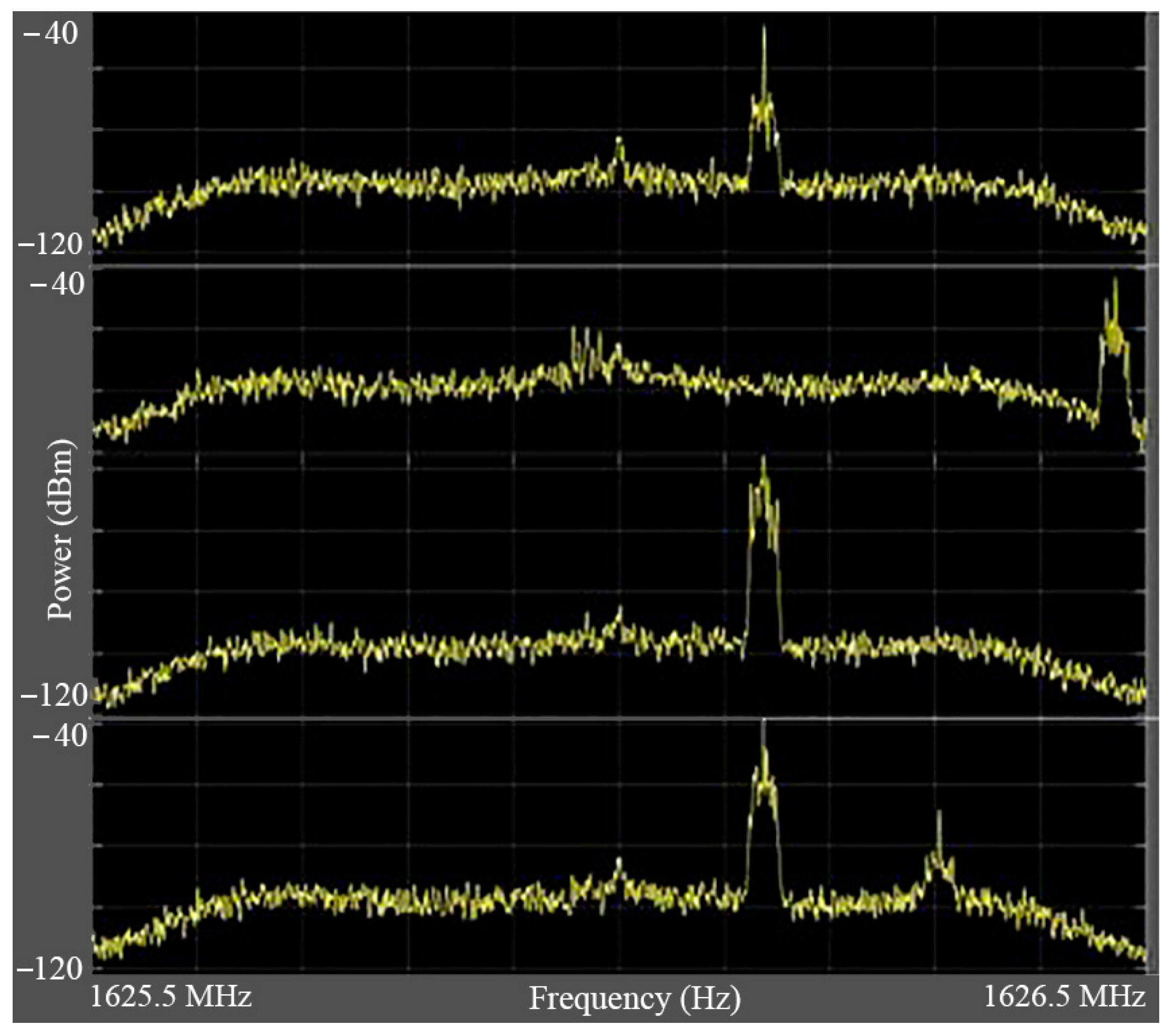
where $v_{m_n}$ and $p_{m_n}$ are the velocity and position of the $n$th satellite of the $m$th LEO constellation, respectively. Additionally, $v_r$ and $p_r$ were defined as the velocity and the position of the receiver, respectively, and $n_{m_n}$ is the measurement noise modeled as a white Gaussian random sequence with variance ${\sigma }_{rrate}$. The variation in the ionospheric and tropospheric delays, $\dot{\delta }{t}_{iono}$ and $\dot{\delta }{t}_{tropo}$, during LEO satellite visibility was negligible compared to the errors in the satellite’s estimated velocities [34]; so, these effects were not mentioned in this article. As depicted in Figure 2, one can observe a different downlink burst from iridium-Next LEO satellites during experimental measures. This experience could also be repeated for Orbcomm, Globalstar, and other VHF/UHF and L-Band LEO satellites. The goal was to observe Doppler shifts and to measure accurately the Doppler frequencies before calculating related pseudorange rates equivalent to the respective measures. It is important to pay attention to the clock bias and the clock drift on the SDR side because they have a direct impact on the estimation accuracy as well as the alignment quality. Although the kinematic and clock states of each observed satellite could be included in the EKF system, our concentration in this study was on deriving the accurate estimation of the receiver’s states. The measurement model for the slave EKF system was defined as Equation (14), where $v\left(k\right)$ is the measurement noise with the zero-mean white Gaussian model. The modeled measurement noise had a variance of ${\sigma }_{m,n}^2$, $m=1,\dots ,M,$ and $n=1,\dots ,N$ where M is the total number of constellations and N is number of the satellites in each one. Additionally, $y\left(k\right)$ is the estimated measurement vector, and z is the pseudorange rate measurement vector obtained from the MC-SDR, given by Equation (15).

$$y\left(k\right)=Hx\left(k\right)+v\left(k\right),$$

(14)

$$z\equiv {\left[\dot{{\rho }_{1_1}},\dots ,\dot{{\rho }_{m_n}}\right]}^T,$$

(15)

Moreover, the measurement matrix $H$ was obtained using the Jacobian matrix of the nonlinear measurement function $h\left(x\left(k\right)\right)$. Finally, the matrix $H$ is given by Equation (16).

$$H=\left[\begin{array}{ccccc}{0}_{1\times 4}& h_{p_{1,1}}^T& -h_{v_{1,1}}^T& 0& c\\ ⋮& ⋮& ⋮& ⋮& ⋮\\ 0_{1\times 4}& h_{p_{1,n}}^T& -h_{v_{1,n}}^T& 0& c\\ ⋮& ⋮& ⋮& ⋮& ⋮\\ 0_{1\times 4}& h_{p_{m,n}}^T& -h_{v_{m,n}}^T& 0& c\end{array}\right],$$

(16)

where c is speed of the light; $h_{p_{m,n}}$ and $h_{v_{m,n}}$ are defined in Equations (17)–(19).

$$h_{p_{m,n}}=\frac{\Delta v_{m_n}{\Vert \Delta p_{m_n}\Vert }_2-\left(\Delta v_{m_n}^T\Delta p_{m_n}\right)\Delta p_{m_n}}{{\Vert \Delta p_{m_n}}_2^3},$$

(17)

$$h_{v_{m,n}}=\frac{\Delta p_{m_n}}{|\Delta p_{m_n}{|}_2},$$

(18)

$$\Delta p_{m_n}=\left[p_r-p_{m_n}\right]\hspace{1em}\Delta v_{m_n}=\left[v_{m_n}-v_r\right],$$

(19)

2.2.3. EKF Update Process

After defining the EKF measurement and the state-space model, the prediction and update processes were required to estimate the receiver’s states. First, the attitude, position, and velocity of the receiver were predicted using the kinematic INS equations, which were discussed previously. Additionally, the clock states of the receiver were predicted using the receiver’s clock bias state-space model. The predicted covariance matrix was obtained by Equation (20).

$$P_{k+1|k}=F_k{P}_{k|k}{F}_k^T+Q_k,$$

(20)

where $F_k$ was obtained using the Jacobian of the INS equations, and $Q_k$ is the covariance of the process noise. The matrix $Q_k$ is defined as $diag\left[Q_{ins},c^2{Q}_{clk}\right]$ in which $Q_{clk}$ is described in Equation (12); $Q_{ins}$ is implemented as the covariance of dynamic disturbance noise in a standard INS kinematics (refer to [30]). Second, the receiver’s states were updated using the Kalman gain, $K_k$, and the pseudorange-rate measurements of LEO satellites, $z$. Finally, the covariance matrix and the Kalman gain were updated. Equations (21)–(23) showed the updated EKF process.

$$x_{k+1|k+1}=x_{k+1|k}+K_{k+1}\left[z_{k+1}-H_{k+1}{x}_{k+1|k}\right],$$

(21)

$$P_{k+1|k+1}=P_{k+1|k}-K_{k+1}{H}_{k+1}{P}_{k+1|k},$$

(22)

$$K_{k+1}=P_{k+1|k}{H}_{k+1}^T{\left[H_{k+1}{P}_{k+1|k}{H}_{k+1}^T+R_{k+1}\right]}^{-1},$$

(23)

where R is the covariance of the measurement noise. As mentioned before, the EKF-based slave system estimates the receiver’s states using the above measurement model and the known orbital data of LEO satellites. These estimated states and the estimated states of the master INS will be the main source of the alignment system. The INS alignment system is totally investigated in the following part.

3. LEO/INS Alignment Architecture

3.1. KF-Based Alignment Method

The receiver’s error model consists of attitude, position, and velocity errors, as well as errors of the gyroscope and the accelerometer. The error model is given by Equation (24).

$$\dot{X}\left(t\right)=F\left(t\right)X\left(t\right)+w\left(t\right),$$

(24)

There are 15 states for the matrix X(t), which defined $\delta \phi$, $\delta \theta$, and $\delta \psi$ as errors of attitude; $\delta v_N$, $\delta v_E$, and $\delta v_D$ as errors of velocity; $\delta L$, $\delta l$, and $\delta h$ as errors of position; $b_{gx}$, $b_{gy},$ and $b_{gz}$ as bias errors of the gyroscope; and finally $b_{ax}$, $b_{ay},$ and $b_{az}$ as bias errors of the accelerometer (see Equation (25)). Moreover, the $w\left(t\right)$ is the white Gaussian noise vector defined for the sensor biases. The evolution of the biases was modeled with a random walk process, where ${\dot{b}}_g={\mu }_g$ and ${\dot{b}}_a={\mu }_a$ with a zero expected value and a covariance of ${\sigma }_{{\mu }_g}^2$ and ${\sigma }_{{\mu }_a}^2$, respectively. The completed states of the model are shown in the vector $X$(t).

$$X\left(t\right)={\left[\delta {\mathsf{\Omega }}^T\delta v^T\delta p^T{b}_g^T{b}_a^T\right]}^T,$$

(25)

where $\delta \mathsf{\Omega }={\left[\delta \varphi \delta \theta \delta \psi \right]}^T$, $\delta v={\left[\delta v_N\delta v_E\delta v_D\right]}^T$, $\delta p={\left[\delta L\delta l\delta h\right]}^T$, $b_g={\left[b_{gx}{b}_{gy}{b}_{gz}\right]}^T$, and $b_a={\left[b_{ax}{b}_{ay}{b}_{az}\right]}^T$. Moreover, the matrix F(t) is defined in Appendix A. The measurement model is $Y\left(t\right)=HX\left(t\right)+n\left(t\right)$, where n(t) is the measurement noise with the white Gaussian model. As described before, the measurements were obtained from the comparison of master and slave positioning systems, which are based on two different sources, namely, LEO downlinks and the IMU data. The measurement matrix H was given by Equation (26). The measurement vector was defined as $Y={\left[\delta \mathsf{\Omega }\delta v\delta p\right]}^T$, where its elements were given by Equation (27).

$$H=\left[\begin{array}{cc}{I}_{9\times 9}& 0_{9\times 6}\end{array}\right],$$

(26)

$$\delta \mathsf{\Omega }={\mathsf{\Omega }}_c-{\mathsf{\Omega }}_s,\delta v=v_c-v_s,\delta p=p_c-p_s,$$

(27)

It should be mentioned that the ${\mathsf{\Omega }}_c$ and ${\mathsf{\Omega }}_s$ were obtained from their quaternion form using the quaternion to Euler transform equation. After discretizing the continuous error model, a linear Kalman filter was implemented to estimate the error states. The Kalman-filter-updated equations had the same process as Equations (20)–(23).

3.2. Observability Analysis and IMU Rotation Simulation

The importance of observability analysis was a clear fact because of its direct effect on the state estimation, and in the second layer it could have influence on the error correction and final results of the navigation system. In the time-variant systems, the observability rank could be measured by the Grammian matrix using the piece-wise constant system (PWCS) method. However, in the systems that have short interval variations, the PWCS method proved that by calculating the stripped observability matrix (SOM), the rank of observability could be defined [35]. For the discussed system included (F, H), the observability matrix in the interval $\left(t_i,t_{i+1}\right)$ was calculated as Equation (28) [36].

$$Q_i={\left[{\left(H\right)}^T,{\left(HF\left(t_i\right)\right)}^T,{\left(H{F}^2\left(t_i\right)\right)}^T,\dots ,{\left(H{F}^{n-1}\left(t_i\right)\right)}^T\right]}^T,$$

(28)

From the PWCS method, the SOM matrix will be obtained as Equation (29).

$$SOM={\left[\begin{array}{cccc}{Q}_1^T& Q_2^T& \cdots & Q_i^T\end{array}\right]}^T,$$

(29)

The rank of the SOM matrix will determine the rank of observability in the error models. Before making our SOM matrix, the rotation algorithm should be determined, and each i-axis rotation showed one time interval. The rotation algorithm is shown in Figure 3, and

Table 1. IMU rotation sequences.

	x-axis ($\mathit{\phi }$)	y-axis ($\mathit{\theta }$)	z-axis ($\mathit{\psi }$)
Interval 1 (initial position)	0°	0°	0°
Interval 2 (1st rotation)	0°	0°	$\pm 180$°
Interval 3 (2nd rotation)	0°	$\pm 180$°	0°

defines each step. Each rotation step was specialized with code number 1. Each step of the Figure 3 can be considered as an interval in the SOM matrix. The rank of observability was calculated before the rotation with the Grammian matrix in a non-rotational IMU platform. The rank of observability for the error model was shown as ${\left[\begin{array}{cccc}H& HF& \cdots & H{F}^{n-1}\end{array}\right]}^T=10$. However, the result of the SOM matrix after the rotation showed the observability rank of 14, which means that from the 15-state system, 14 states could be observed that demonstrated a great enhancement in comparison with the works done in [15] due to the minimum rotation steps. The presented rotation sequence was based on the optimized dual-axis rotational IMU motion for strapdown INS (SINS) (refer to [37]).

As illustrated above, the IMU was rotated around its z and y axes. For each rotation, there was a transform matrix, which changed the biases in the body frame. The output of the accelerometer and the gyroscope after performing the mentioned rotations were modeled as Equations (30) and (31), where ${\epsilon }^b$ and ${\epsilon }^q$ were defined as IMU bias vectors in the body frame and the new IMU frame after the rotation, respectively. As a result of that, $C_q^b$ was the transform matrix from the IMU frame to the body frame.

$${\epsilon }^b=C_q^b{\epsilon }^q,$$

(30)

$$C_q^b=\left[\begin{array}{ccc}cos\left(\psi \right)& sin\left(\psi \right)& 0\\ -sin\left(\psi \right)& cos\left(\psi \right)& 0\\ 0& 0& 1\end{array}\right]\left[\begin{array}{ccc}cos\left(\theta \right)& 0& -sin\left(\theta \right)\\ 0& 1& 0\\ sin\left(\theta \right)& 0& cos\left(\theta \right)\end{array}\right]=\left[\begin{array}{ccc}cos\left(\psi \right)cos\left(\theta \right)& sin\left(\psi \right)& -cos\left(\psi \right)sin\left(\theta \right)\\ -sin\left(\psi \right)cos\left(\theta \right)& cos\left(\psi \right)& -sin\left(\psi \right)sin\left(\theta \right)\\ sin\left(\theta \right)& 0& cos\left(\theta \right)\end{array}\right],$$

(31)

The IMU biases were obtained by Equations (32) and (33).

$$b_g^b=\left[\begin{array}{c}{b}_{gx}^{q}cos\left(\psi \right)cos\left(\theta \right)+b_{gy}^{q}sin\left(\psi \right)-b_{gz}^{q}cos\left(\psi \right)sin\left(\theta \right)\\ -b_{gx}^{q}sin\left(\psi \right)cos\left(\theta \right)+b_{gy}^{q}cos\left(\psi \right)-b_{gz}^{q}sin\left(\psi \right)sin\left(\theta \right)\\ b_{gx}^{q}sin\left(\theta \right)+b_{gz}^{q}cos\left(\theta \right)\end{array}\right],$$

(32)

$$b_a^b=\left[\begin{array}{c}{b}_{ax}^{q}cos\left(\psi \right)cos\left(\theta \right)+b_{ay}^{q}sin\left(\psi \right)-b_{az}^{q}cos\left(\psi \right)sin\left(\theta \right)\\ -b_{ax}^{q}sin\left(\psi \right)cos\left(\theta \right)+b_{ay}^{q}cos\left(\psi \right)-b_{az}^{q}sin\left(\psi \right)sin\left(\theta \right)\\ b_{ax}^{q}sin\left(\theta \right)+b_{az}^{q}cos\left(\theta \right)\end{array}\right],$$

(33)

In a 2$\pi$ cycle, the elements of $b_g^b$ and $b_a^b$, which have a single sine or cosine function, are removed. The rotation sequence could be repeated several times during the real experiments. This motion could be implemented by simulation or using a rotatory platform connected to the IMU [38].

4. Iridium-Next and Orbcomm Downlink Signal Specification

Usually, LEO satellites use quadrature phase shift keying (QPSK) or code-division multiple access (CDMA) downlink signals, which can be of two main types: continuous (such as Orbcomm and Globalstar) and burst-based (such as Iridium, etc.). In this study, we concentrated on two outstanding constellations, namely, Orbcomm and Iridium-NEXT. The orbital data of each satellite in all three constellations were updated every day in a TLE file, which is freely downloadable from the North American Aerospace Defense Command (NORAD) website. The data are represented with one of the simplified perturbations models such as SGP, SGP4, and SGP8.

All the Orbcomm satellites propagate a continuous packed data in 1 MHz of the VHF bandwidth frequency between 137 to 138 MHz. The bit rate of the transmitted downlinks is 4800 bps. Technically, a major frame of Orbcomm downlinks includes 16 minor frames. Each 600 words is defined as a minor frame. These satellites transmit on 15 different center frequencies separated by a 25 KHz protected band among them. Although not all of the Orbcomm satellites are functional, there are eleven channels that definitely transmit downlink signals. Every single Orbcomm satellite vehicle transmits on two downlink frequencies in the mentioned VHF band [39]. On the other side, the Iridium-Next constellation works on the L-band frequency range. The frequency of their transmitted signals is designed on 1616 to 1626.5 MHz for both duplex and simplex channels. These downlinks are being propagated in 30 duplex sub-bands between 1616 and 1626 MHz. Additionally, there are 12 simplex channels between 1626 and 1626.5 MHz, with 90 ms time division multiple-access (TDMA) frames. Both simplex and duplex signals are based on burst messages; however, the simplex bursts are more suitable for navigation applications. The reason is the fact that they are always being transmitted from Iridium satellites. The center frequency of the Iridium-NEXT ring alert is 1626.27833 MHz and those of messaging channels are 1626.437500 MHz, 1626.395833 MHz, 1626.145833 MHz, and 1626.104167 MHz, for primary, secondary, tertiary, and quaternary messaging channels, respectively [40].

5. Experimental Evaluation and Results

To assess the proposed LEO/SOP-based INS alignment method, two different experiments were designed and performed. The goal of both experiments was to estimate the trajectory of an aerial vehicle. The first experiment was implemented by a ground vehicle, while the second one was performed using a light aircraft. This section includes two body parts. First, we describe the hardware and software configuration and specifications of each experiment. Second, the observed satellite and outputs of the receiver are investigated for each experiment. Finally, the experimental results of the proposed method are discussed in detail.

5.1. Hardware and Software Configuration

5.1.1. Ground Experiment

The location of the experiment was in the city of Montreal with a ground vehicle equipped by the MC-SDR and an IMU. The principal goal of this experiment was to acquire the SOP downlinks transmitted by multiple LEO satellites to aid the EKF-based slave Doppler positioning system. A 9 degree-of-freedom (DoF) VN-100 IMU was mounted on the ground vehicle to record the vehicle’s three-axis acceleration, three-axis magnetic field, and three-axis angular velocity as a dynamic receiver. To receive precise downlink signals, the antennas from each constellation were prepared based on our last signal acquisition tests in various environments. As a result, a dual-band VHF/UHF mobile Orbcomm as well as an Iridium-Next L-band antenna were connected to two different SDRs: a BladeRF V2.0 and a RTL-SDR dongle. First, the overhead satellites were detected using their predicted elevation angles. Later, the SDRs recorded the satellite’s downlinks from the Iridium-NEXT and the Orbcomm constellations.

To have an acceptable and noise-free signal acquisition, we used a RF bandpass filter on the Orbcomm signals and a low-noise amplifier (LNA) for the Iridium-NEXT channel. The recording sampling frequency for the IMS was set to 100 Hz and that of the SDRs was selected at 1.2288 MHz. The center frequencies of the Orbcomm and Iridium-NEXT channels were specified at 137.5 MHz and 1626 MHz, respectively. Figure 4 demonstrates the overall details of the utilized hardware and software during the experiment. The LASSENA MC-SDR was used to analyze the signals. It also obtained the pseudorange rate measurements of the detected overhead satellites. At the end, the inertial data and the doppler shift outputs of the receiver were postprocessed in the MATLAB to run the proposed alignment method.

5.1.2. Flight Experiment

The flight experiment was performed in the Joliette airport near the Montreal City. A light aircraft was equipped with a Novatel GNSS/INS RTK connected to two GNSS antennas. An Iridium-Next L-band antenna was used to record the Iridium downlinks during the flight. The utilized front-end and the LNA were the same as the ground experiment. The position output of the RTK was considered as the true reference trajectory. The receiver’s sampling frequency and bandwidth were also followed by the specifications of the ground test. The time duration of the flight test was 10 min. The GNSS measurements were blocked after 5 min of the experiment. More details about the overhead satellites and the Doppler shift measurements are discussed later. Figure 5 shows the installed antennas for the LEO satellites as well as the GNSS receiver in the aircraft.

5.2. Doppler Shift Measurements

5.2.1. Ground Experiment

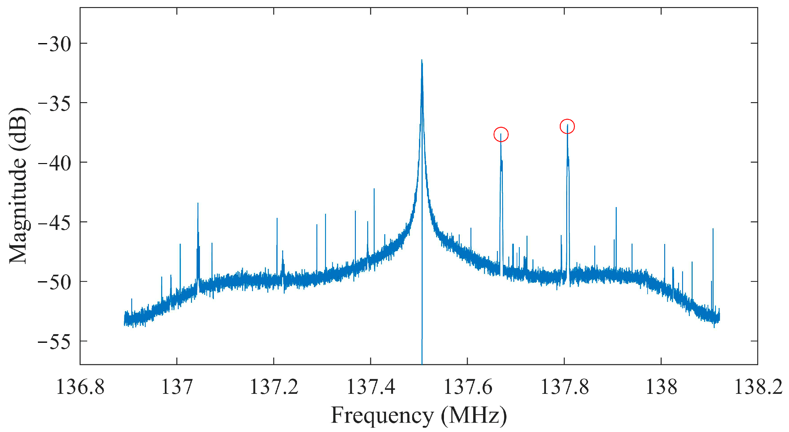
The experiment was done on the 6 November 2020 in Montreal, Canada. During the experiment, one Orbcomm (Orbcomm FM-113) and one Iridium-NEXT (Iridium 141) satellite were visible in the receiver’s sight. The TLE files of the observed satellites were downloaded from the American NORAD website on the day of the experiment. To detect the overhead satellites, we implemented a real-time power spectral density (PSD) viewer on MATLAB for both RTL-SDR and BladeRF software-defined radios. Our latest experiments showed that in each time at least one Iridium satellite was visible above the Montreal city and its vicinity. As a result of that, we started the experiment when an Orbcomm satellite was detected on the PSD viewer. Figure 6 shows a geographical view of the overhead satellite as well as the location of the airport. It also presents the estimated Doppler shifts of the Iridium satellite in three different channels (quaternary, primary, and ring alert). Figure 7 demonstrates the PSD analysis of the Orbcomm channel. The receiver detected two frequency peaks with magnitudes of more than −38 dB. These frequencies were 137.6626 and 137.80 MHz, which are the dual transmitted frequencies of the Orbcomm space vehicle (SV) FM-113. Later, the Doppler shift of each satellite was tracked using the MC-SDR for the entire trajectory. Although the Doppler shift of the Orbcomm on its two frequencies was obtained, just that of the higher frequency (137.80 MHz) was considered for this study. It should be mentioned that the receiver showed the same Doppler behaviors for both carrier frequencies as they were propagated from the same satellite origin. For the Iridium channels, the Doppler shifts tracked in all the three channels had the same behavior. However, it can be seen that the Doppler shifts given by the quaternary messaging channel showed better quality with more dense measurements, which is more suitable for the EKF-based alignment method.

To validate the obtained Doppler shifts, we used the LASSENA’s Doppler simulator based on the simplified perturbation (SGP, SGP4, and SGP8) model. In the simulation, regarding the fact that the vehicle’s velocity related to that of the satellite was a small value, the satellite’s velocity was considered as a relative velocity between the satellite and the receiver. It could provide us with an estimation of the Doppler shift from each satellite during the experiment. The estimated Doppler shifts for the Orbcomm FM 113 and the Iridium 141 satellites were continuous and burst-based, respectively. Figure 8 shows the comparison of the simulated and the estimated Doppler-shift curves. It was obvious that the receiver could extract the Doppler shifts from the LEO satellites with high accuracy. The accuracy of the receiver for different channels and constellations were previously discussed in [6].

5.2.2. Flight Experiment

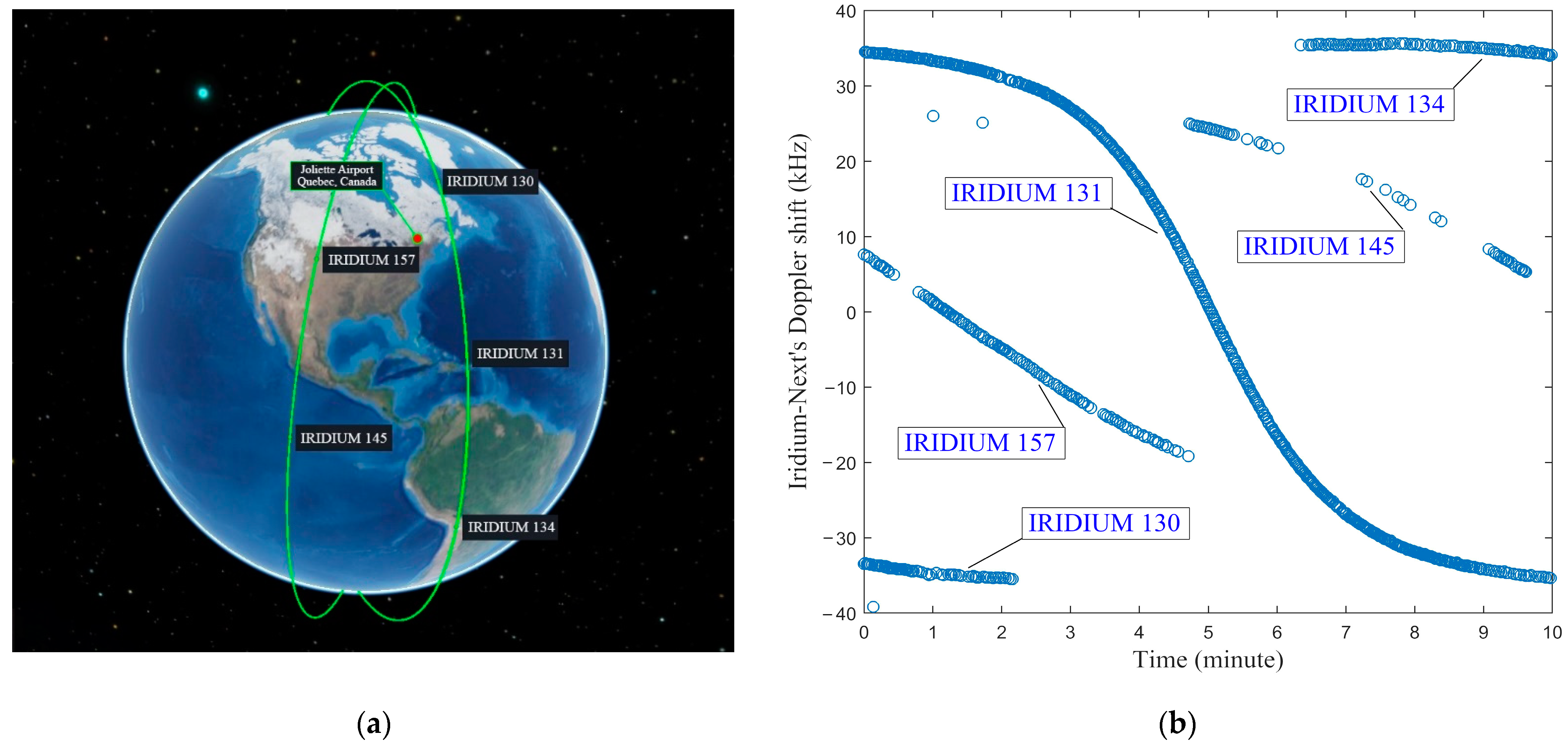
The flight experiment was on 14 April 2021. During the 10 min of the experiment, five Iridium-Next satellites were observed in two different planes. The downlink bursts of these satellites, Iridium-130, Iridium-131, Iridium-134, Iridium-145, and Iridium-157, were acquired using the MC-SDR. Figure 9 shows the tracked Doppler shifts during the entire trajectory. The Doppler shifts were acquired in the quaternary messaging channel as it was the most powerful and dense measurement obtained by the receiver. The resolution of the Doppler shift was different for satellites in various orbital planes. In this case, the transmitted messaging bursts from Iridium 130, 131, and 134 were in a range of around −40 kHz to 40 kHz; however, this range for the Iridium 157 and 145 was between −20 kHz to 20 kHz. The distance of each orbital plane led different elevation angles seen by the receiver. Additionally, the quality of the measurement acquired by the satellites in the closer plane was much better, as depicted in Figure 9. This means that the satellites located on the closer plane pass the receiver’s location with a maximum elevation angle of ${62.3}^{\circ }$; however, the elevation angle for satellites of the other plane was at a maximum at ${21.5}^{\circ }$. Figure 9 also represents the orbit path of the satellites and the receiver’s location.

5.3. Experimental Results and Discussion

5.3.1. Ground Experiment

The mentioned hardware and software equipment was installed on a ground vehicle, and the experiment was done in a pre-selected route with 166 s duration. The EKF-based slave model was injected using the pseudorange rate measurements of two satellites from the two different constellations (Orbcomm and Iridium-NEXT) given by the receiver. The slave system also utilized the position and velocity of both satellites obtained from the downloaded TLE files. Additionally, the GPS was used to initialize the system and record the reference position track. The true reference orientation was also recorded by the AHRS module of the VN100-Rugged IMU. The initial covariance matrices were defined as $P_x\left(0|0\right)=diag\left[{10}^{-4}.I_{4\times 4},{10}^{-2}.I_{6\times 6},10,2\right]$, for the slave EKF system, and $P_X\left(0|0\right)=diag\left[{10}^{-10}.I_{3\times 3},{10}^{-6}.I_{6\times 6},{10}^{-2}.I_{3\times 3},{10}^{-3}.I_{3\times 3}\right]$ for the KF alignment system, where, I is the identity matrix. In the receiver’s model, a typical temperature-compensated crystal oscillator (TCXO) was considered, with coefficient values $\left\{h_{0,r},h_{-2,r}\right\}=\left\{9.4\times {10}^{-21},3.8\times {10}^{-21}\right\}$.

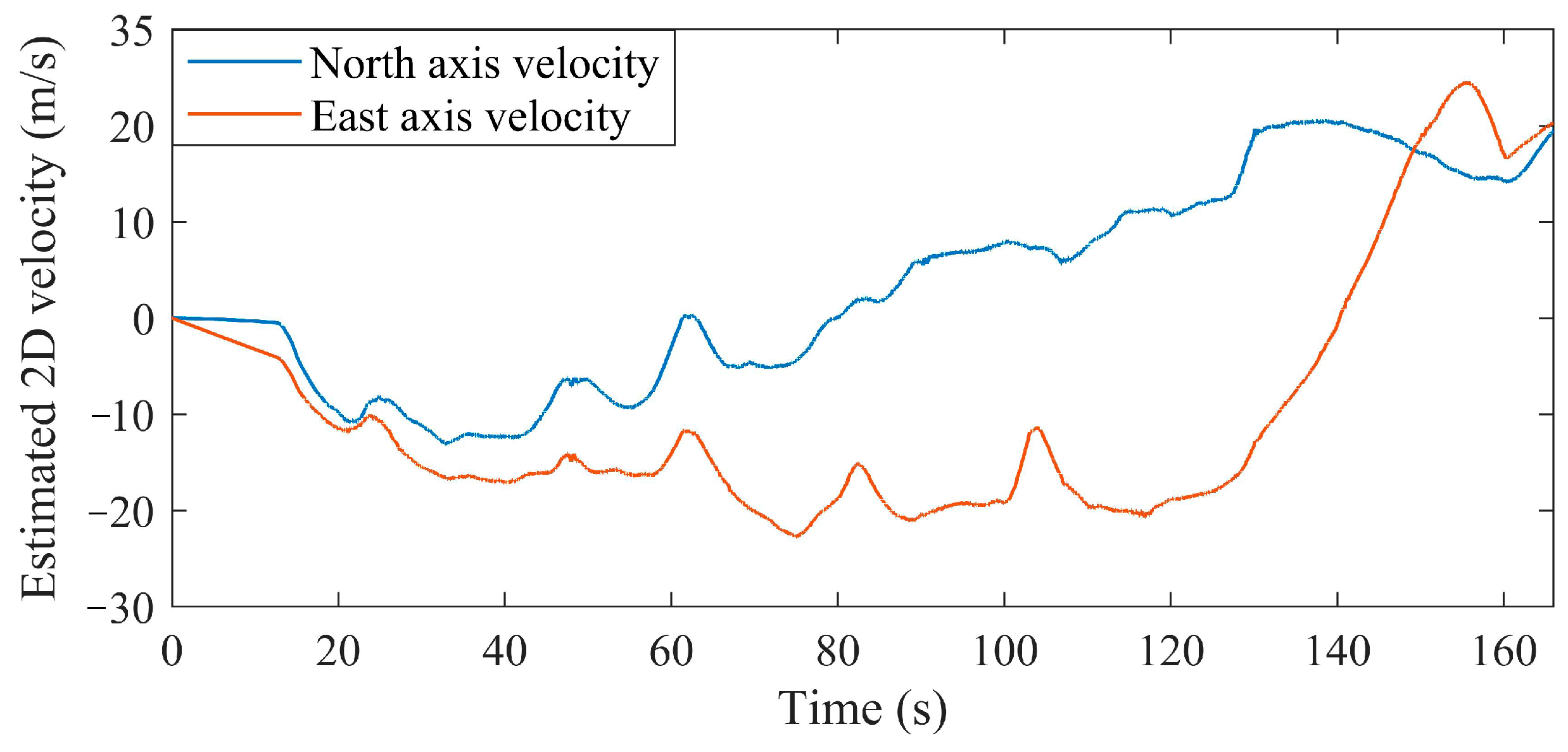
Figure 10 demonstrates the comparison of the reference and estimated AV’s orientation obtained from the proposed alignment and positioning algorithm. The mean square error (MSE) for the roll, pitch, and heading angles during the experiment were obtained as ${2.0234}^{\circ }$, ${1.9764}^{\circ }$, and ${22.1529}^{\circ }$, respectively. Furthermore, Figure 11 shows the attitude errors. It was obvious that the highest attitude error was for the heading angle, while it diverged gradually by time. In this case, cutting off the GNSS had a significant effect on the heading drift; moreover, attitude calibration using the proposed SOP-based method could bound the roll and pitch errors with higher precision. Figure 12 represents the estimated velocity of the AV during the experiment, visualized in the local navigation frame.

The receiver’s clock errors were estimated for the typical TCXO using the slave system, as depicted in Figure 13. The clock error parameters were increased after a downward peak, which is caused by the satellite’s pass. The clock bias reached its highest value, at about 300 m, and the clock drift culminated at around 1.5 m/s. Figure 14 shows the final 2-D position results plotted on the geographical map with latitude and longitude axes. The results prove that the proposed alignment method was able to bound the stand-alone INS. On the other hand, the INS was well-calibrated using the pseudorange rate measurements of the LEO satellites and the observability enhancement method based on the IMU rotation. The proposed method showed the root mean square (RMS) error of 12.234 m in the entire trajectory, which is a significant advance compared to the stand-alone INS mode. The end-to-end error in the INS mode was also about 245.23 m, while this error after performing the proposed alignment method decreased to a mere 9.2 m.

5.3.2. Flight Experiment

The obtained pseudorange rate measurement from the five overhead satellites led at least two and a maximum of three measurements during the entire trajectory. In the first seconds of the experiment, the aircraft took off from the Joliette airport, and it followed a challengeable trajectory. The GNSS receiver recorded the true reference position of the flight vehicle; however, the algorithm did not utilize the measurements of the GNSS receiver after 5 min. The last 5 min of the trajectory were estimated using multi-satellite LEO-SOP pseudorange rate measurements. Figure 15 demonstrates the true and estimated position of the aircraft, highlighting the GNSS-blocked point and visualizing the experiment’s region on a 3-D geographical map. The figure was plotted using the mapping toolbox of the MATLAB.

Figure 16 shows the North and East errors of the proposed alignment method along with $\pm 3\sigma$ bounds. The red dash line illustrates the GNSS cut-off point. The flight experiment was able to measure the stability of the system in medium-term durations. It can be seen that by the variation of the aircraft’s attitude, the position error increased gradually. Overall, the method bounded the error of the INS by the SOP-aided alignment system.

Table 2. RMSE of the alignment method for different time slots from the start point compared with the error of the Doppler positioning method.

	5′:30″~6′:00″	5′:30″~7′:00″	5′:30″~8′:00″	5′:30″~9′:00″	5′:30″~10′:00″
Duration from start point	30 s	1.5 min	2.5 min	3.5 min	4.5 min
RMSE (m) Doppler positioning	80.9458	110.9693	151.5803	224.4044	550.2049
RMSE (m) SOP-aided alignment	16.1054	35.6654	56.1978	282.1078	196.7429

shows the root mean square error (RMSE) of the proposed method in different time slots. The goal was to measure the stability and the resiliency of the system in longer terms. As mentioned before, the GNSS was blocked after 5 min and 30 s from the start point of the experiment. The RMSE in the first 1.5 min of the experiment was 35.6654 m, and after 1 min it reached 56.1978 m. Then, it culminated at 372.1078 m in the next minutes. The RMSE of the entire trajectory for 4.5 min of the experiment was 196.7429 m. Figure 17 illustrates the estimated bias of the IMU, and Figure 18 shows the estimated orientation of the aircraft.

6. Conclusions

LEO-SOPs with a wide-carrier frequency rage, a number of satellites, and an orbit time are somehow known as free infrastructures for augmenting the outdoor navigation systems in non-GNSS environments. The use of pseudorange rate measurements of downlink signals propagated from Iridium-Next and Orbcomm constellations are popularly investigated in many previous works, although most of them showed the navigation performance in short-term experiments. In this study, a regular LEO-based Doppler positioning method was used as a slave EKF estimator to calibrate the INS system. The error state space model of the INS was presented as a master system. In parallel, two EKFs were presented in the proposed method. At first, the slave EKF estimates the position of the vehicle by fusing the pseudorange rate measurements obtained from the receiver. By comparing the positions of the master and the slave systems, the error measurements were provided for the INS alignment model. This system calculated all the errors of the INS system including IMU biases and errors of the position, the velocity, and the attitude. As the alignment model was not completely observable, the observability rank of the system was increased by rotation of the IMU in a special sequence. The observability rank of the calibration model was enhanced to 14 out of 15 states.

Two experiments were planned to examine the proposed method. The receiver, antenna, front-ends, IMU, and other equipment were installed one time on the ground and the next time on a flight vehicle. A special 2-min trajectory for the ground experiment and a 10-min air path for the flight test were selected. The final accuracy of the ground test reached 12.234 m, which showed a significant improvement compared to the stand-alone INS. The results of the flight test were demonstrated in different time periods. It helped us to track the accuracy of the proposed method by time. It could also measure the robustness of each algorithm. The accuracy of the alignment method in the first 150 s increased by around 60% compared to the Doppler positioning method. The method showed a RMSE of around 197 m, which advanced around 180% for the entire trajectory.

References

- Yu, M.-J. INS/GPS Integration System Using Adaptive Filter for Estimating Measurement Noise Variance. IEEE Trans. Aerosp. Electron. Syst. 2012, 48, 1786–1792. [Google Scholar] [CrossRef]
- Zhong, M.; Guo, D.; Guo, J. PMI Based Nonlinear H∞ Estimation of Unknown Sensor Error for INS/GPS Integrated System. IEEE Sens. J. 2014, 15, 1. [Google Scholar] [CrossRef]
- Falco, G.; Pini, M.; Marucco, G. Loose and Tight GNSS/INS Integrations: Comparison of Performance Assessed in Real Urban Scenarios. Sensors 2017, 17, 255. [Google Scholar] [CrossRef] [PubMed]
- Zheng, L.; Xue, R. Signals of Opportunity Navigation Methods for Complex Lower Airspace Flight. In Proceedings of the 2011 IEEE 5th International Conference on Cybernetics and Intelligent Systems (CIS), Qingdao, China, 17–19 September 2011; pp. 272–276. [Google Scholar] [CrossRef]
- Khalife, J.J.; Kassas, Z.M. Receiver design for Doppler positioning with LEO satellites. In Proceedings of the ICASSP 2019-2019 IEEE International Conference on Acoustics, Speech and Signal Processing (ICASSP), Brighton, UK, 12–17 May 2019; pp. 5506–5510. [Google Scholar]
- Farhangian, F.; Landry, R. Multi-constellation software-defined receiver for Doppler positioning with LEO satellites. Sensors 2020, 20, 5866. [Google Scholar] [CrossRef] [PubMed]
- Morales, J.J.; Roysdon, P.F.; Kassas, Z.M. Signals of Opportunity Aided Inertial Navigation. In Proceedings of the 29th International Technical Meeting of the Satellite Division of the Institute of Navigation (Ion Gnss + 2016), Portland, OR, USA, 12–16 September 2016; pp. 1492–1501. [Google Scholar] [CrossRef] [Green Version]
- Morales, J.J.; Khalife, J.; Kassas, Z.M. Collaborative Autonomous Vehicles with Signals of Opportunity Aided Inertial Navigation Systems. In Proceedings of the 2017 International Technical Meeting of The Institute of Navigation, Monterey, CA, USA, 30 January–2 February 2017; pp. 805–818. [Google Scholar] [CrossRef] [Green Version]
- Morales, J.J.; Kassas, Z.M. Distributed Signals of Opportunity Aided Inertial Navigation with Intermittent Communication. In Proceedings of the 30th International Technical Meeting of the Satellite Division of The Institute of Navigation (ION GNSS+ 2017), Portland, OR, USA, 29 September 2017; pp. 2519–2530. [Google Scholar] [CrossRef] [Green Version]
- Benzerrouk, H.; Nguyen, Q.; Xiaoxing, F.; Amrhar, A.; Nebylov, A.V.; Landry, R. Alternative PNT Based on Iridium Next LEO Satellites Doppler/INS Integrated Navigation System. In Proceedings of the 2019 26th Saint Petersburg International Conference on Integrated Navigation Systems (ICINS), Saint Petersburg, Russia, 27–29 May 2019; pp. 1–10. [Google Scholar] [CrossRef]
- Tan, Z.; Qin, H.; Cong, L.; Zhao, C. Positioning Using IRIDIUM Satellite Signals of Opportunity in Weak Signal Environment. Electronics 2020, 9, 37. [Google Scholar] [CrossRef] [Green Version]
- Acebes Cebrian, C. Opportunistic Navigation with Iridium next LEO Satellites. Bachelor’s Thesis, Universitat Politècnica de Catalunya, Barcelona, Brazil, 2020. [Google Scholar]
- Thompson, S.; Martin, S.; Bevly, D. Single Differenced Doppler Positioning with Low Earth Orbit Signals of Opportunity and Angle of Arrival Estimation. In Proceedings of the 2021 International Technical Meeting of The Institute of Navigation, Online, 25–28 January 2021; pp. 497–509. [Google Scholar]
- Orabi, M.; Khalife, J.; Kassas, Z.M. Opportunistic navigation with Doppler measurements from Iridium Next and Orbcomm LEO satellites. In Proceedings of the 2021 IEEE Aerospace Conference (50100), Big Sky, MT, USA, 6–13 June 2021; pp. 1–9. [Google Scholar]
- Bo, X.; Feng, S. A FOG Online Calibration Research Based on High-Precision Three-Axis Turntable. In Proceedings of the 2009 International Asia Conference on Informatics in Control, Automation and Robotics, Bangkok, Thailand, 1–2 February 2009; pp. 454–458. [Google Scholar] [CrossRef]
- Ahn, H.-S.; Won, C.-H. Fast Alignment Using Rotation Vector and Adaptive Kalman Filter. IEEE Trans. Aerosp. Electron. Syst. 2006, 42, 70–83. [Google Scholar] [CrossRef]
- Li, Y.; Zhu, X.; Liu, H. Shaft Orientation Calibration Method for Single-Axis Rotation INS. In Proceedings of the 2019 Chinese Control Conference (CCC), Guangzhou, China, 27–30 July 2019; IEEE: Piscataway, NJ, USA, 2019; pp. 7115–7119. [Google Scholar] [CrossRef]
- Zha, F.; Chang, L.; He, H. Comprehensive error compensation for dual-axis rotational inertial navigation system. IEEE Sens. J. 2020, 20, 3788–3802. [Google Scholar] [CrossRef]
- Lu, Z.; Li, J.; Zhang, X.; Feng, K.; Wei, X.; Zhang, D.; Mi, J.; Liu, Y. A New In-Flight Alignment Method with an Application to the Low-Cost SINS/GPS Integrated Navigation System. Sensors 2020, 20, 512. [Google Scholar] [CrossRef] [PubMed] [Green Version]
- Zhang, H.; Zhang, X. Robust SCKF filtering method for MINS/GPS in-motion alignment. Sensors 2021, 21, 2597. [Google Scholar] [CrossRef] [PubMed]
- Park, J.G.; Kim, J.; Lee, J.G.; Park, C.; Jee, G.; Oh, J.T. The Enhancement of INS Alignment Using GPS Measurements. In Proceedings of the IEEE 1998 Position Location and Navigation Symposium (Cat. No.98CH36153), Palm Springs, CA, USA, 20–23 April 1998; pp. 534–540. [Google Scholar] [CrossRef]
- Wang, L.; Gao, J.; Li, K.; Song, T. Optimization-Based in-Motion Alignment for Rotation INS in GPS-Challenging Environments. In Proceedings of the 2017 IEEE 2nd Advanced Information Technology, Electronic and Automation Control Conference (IAEAC), Chongqing, China, 25–26 March 2017; pp. 1693–1703. [Google Scholar] [CrossRef]
- Liu, X.; Xu, X.; Zhao, Y.; Wang, L.; Liu, Y. An initial alignment method for strapdown gyrocompass based on gravitational apparent motion in inertial frame. Measurement 2014, 55, 593–604. [Google Scholar] [CrossRef]
- Li, Q.; Ben, Y.; Yang, J. Coarse alignment for fiber optic gyro SINS with external velocity aid. Opt. Int. J. Light Electron. Opt. 2014, 125, 4241–4245. [Google Scholar] [CrossRef]
- Liu, X.; Liu, X.; Song, Q.; Yang, Y.; Liu, Y.; Wang, L. A novel self-alignment method for SINS based on three vectors of gravitational apparent motion in inertial frame. Measurement 2015, 62, 47–62. [Google Scholar] [CrossRef]
- Du, S. Rotary Inertial Navigation System with a Low-Cost MEMS IMU and Its Integration with GNSS. Ph.D. Thesis, University of Calgary, Calgary, AB, Canada, 2015. [Google Scholar]
- Zhang, Y.; Zhou, B.; Song, M.; Hou, B.; Xing, H.; Zhang, R. A Novel MEMS Gyro North Finder Design Based on the Rotation Modulation Technique. Sensors 2017, 17, 973. [Google Scholar] [CrossRef] [PubMed] [Green Version]
- Du, S.; Sun, W.; Gao, Y. MEMS IMU error mitigation using rotation modulation technique. Sensors 2016, 16, 2017. [Google Scholar] [CrossRef] [PubMed]
- Collin, J. MEMS IMU carouseling for ground vehicles. IEEE Trans. Veh. Technol. 2015, 64, 2242–2251. [Google Scholar] [CrossRef]
- Titterton, D.H.; Weston, J.L. Strapdown Inertial Navigation Technology, 2nd ed.; IEE Radar, Sonar, Navigation, and Avionics Series 17; Institution of Electrical Engineers: Stevenage, UK, 2004. [Google Scholar]
- Kassas, Z.; Humphreys, T. Observability analysis of collaborative opportunistic navigation with pseudorange measurements. IEEE Trans. Intell. Transp. Syst. 2014, 15, 260–273. [Google Scholar] [CrossRef]
- Thompson, A.R.; Moran, J.M.; Swenson, G.W., Jr. Interferometry and Synthesis in Radio Astronomy; Springer Nature: Cham, Switzerland, 2017. [Google Scholar]
- Groves, P. Principles of GNSS, Inertial, and Multisensor Integrated Navigation Systems, 2nd ed.; Artech House: Norwood, MA, USA, 2013. [Google Scholar]
- Enge, P.K. The global positioning system: Signals, measurements, and performance. Int. J. Wirel. Inf. Netw. 1994, 1, 83–105. [Google Scholar] [CrossRef]
- Feng, S.; Qian, S.; Yueyang, B.; Ya, Z.; Gao, W. A New Method of Initial Alignment and Self-Calibration Based on Dual-Axis Rotating Strapdown Inertial Navigation System. In Proceedings of the 2012 IEEE/ION Position, Location and Navigation Symposium, Myrtle Beach, SC, USA, 23–26 April 2021; pp. 808–813. [Google Scholar] [CrossRef]
- Ogata, K. Modern Control Engineering; Prentice Hall: Upper Saddle River, NJ, USA, 1997. [Google Scholar]
- Sun, W.; Xu, A.G.; Che, L.N.; Gao, Y. Accuracy improvement of SINS based on IMU rotational motion. IEEE Aerosp. Electron. Syst. Mag. 2012, 27, 4–10. [Google Scholar] [CrossRef]
- Xing, H.; Chen, Z.; Yang, H.; Wang, C.; Lin, Z.; Guo, M. Self-Alignment MEMS IMU Method Based on the Rotation Modulation Technique on a Swing Base. Sensors 2018, 18, 1178. [Google Scholar] [CrossRef] [PubMed] [Green Version]
- Kenny, M. Ever Wondered What Is on the Orbcomm Satellite Downlink? Available online: http://mdkenny.customer.netspace.net.au/Orbcomm.pdf (accessed on 16 October 2020).
- Manual for ICAO Aeronautical Mobile Satellite (Route) Service, Part 2–IRIDIUM, Draft V4. Available online: https://www.icao.int/safety/acp/Inactive%20working%20groups%20library/ACP-WG-M-Iridium-8/IRD-SWG08-IP05%20-%20AMS(R)S%20Manual%20Part%20II%20v4.0.pdf (accessed on 16 October 2020).
Figure 1.
Block diagram of the proposed in-flight INS alignment method.
Figure 2.
PSD analysis of the Iridium-Next bursts in different time slots.
Figure 3.
3D demonstration of IMU rotation sequences in three steps.
Figure 4.
The ground vehicle and the equipment used in the ground experiment.
Figure 5.
The light aircraft and the equipment used in the flight experiment.
Figure 6.
(a) Geographical view of the overhead satellites. (b) Tracked Doppler shifts from the Iridium 141 in three different channels: quaternary message, primary message, and ring alert.
Figure 7.
Power spectral density (PSD) analysis representation for the transmitted downlinks of Orbcomm FM 113 satellite.
Figure 8.
Estimated and simulated Doppler shifts for (a) Iridium-141 satellite, and (b) Orbcomm FM-113 satellite.
Figure 9.
(a) 3D Earth representation of the overhead Iridium-Next satellites. (b) Doppler shift curve tracked by the receiver.
Figure 10.
The estimated and reference orientation of the ground vehicle for (a) roll angle, (b) pitch angle, and (c) heading.
Figure 11.
The orientation error for (a) roll angle, (b) pitch angle, and (c) heading.
Figure 12.
The estimated velocity of the ground vehicle for the North and East axes.
Figure 13.
(a) The estimated receiver’s clock bias. (b) The estimated receiver’s clock drift.
Figure 14.
The estimated trajectory of the vehicle compared to the stand-alone INS and the true reference position.
Figure 15.
Experimental results include the geographical view of the airport and a comparison of the true and estimated trajectory.
Figure 16.
The North (a) and East (b) position errors of the aircraft before and after blocking the GNSS compared with the error of the Doppler positioning method.
Figure 17.
(a) Estimated accelerometer bias, and (b) Estimated gyroscope bias with bound.
Figure 18.
Estimated attitude of the aircraft with bound.