A Nonlinear Ultrasonic Modulation Method for Crack Detection in Turbine Blades


Materials Research Centre, Department of Mechanical Engineering, University of Bath, Bath BA2 7AY, UK
*
Author to whom correspondence should be addressed.
Aerospace 2020, 7(6), 72; https://doi.org/10.3390/aerospace7060072
Submission received: 17 April 2020
/
Revised: 27 May 2020
/
Accepted: 1 June 2020
/
Published: 4 June 2020
(This article belongs to the Special Issue Selected Papers from IWSHM 2019)
Abstract
:In modern gas turbines, efforts are being made to improve efficiency even further. This is achieved primarily by increasing the generated pressure ratio in the compressor and by increasing the turbine inlet temperature. This leads to enormous loads on the components in the hot gas region in the turbine. As a result, non-destructive testing and structural health monitoring (SHM) processes are becoming increasingly important to gas turbine manufacturers. Initial cracks in the turbine blades must be identified before catastrophic events occur. A proven method is the linear ultrasound method. By monitoring the amplitude and phase fluctuations of the input signal, structural integrity of the components can be detected. However, closed cracks or small cracks cannot be easily detected due to a low impedance mismatch with the surrounding materials. By contrast, nonlinear ultrasound methods have shown that damages can be identified at an early stage by monitoring new signal components such as sub- and higher harmonics of the fundamental frequency in the frequency spectrum. These are generated by distortion of the elastic waveform due to damage/nonlinearity of the material. In this paper, new global nonlinear parameters were derived that result from the dual excitation of two different ultrasound frequencies. These nonlinear features were used to assess the presence of cracks as well as their qualitative sizes. The proposed approach was tested on several samples and turbine blades with artificial and real defects. The results were compared to samples without failure. Numerical simulations were conducted to investigate nonlinear elastic interaction of the stress waves with the damage regions. The results show a clear trend of nonlinear parameters changing as a function of the crack size, demonstrating the capability of the proposed approach to detect in-service cracks.
1. Introduction
Linear ultrasound techniques are a proven method in modern component inspection. Failure detection is carried out here by changes in the elastic properties such as sound velocity, damping, transmission coefficients, and reflection coefficients [1,2,3].
Hikata et al. brought a significant development of this technique in 1965. They found that a sinusoidal ultrasonic wave distorts the fundamental frequency as it propagates in the presence of nonlinearities [4]. An ultrasonic wave propagates into a solid with the fundamental frequency. If this is disturbed during propagation in the body, harmonics are generated. If the amplitudes of these harmonic frequencies are now measured and compared with the fundamental frequencies, these comparative values are a good indicator for detecting changes in the material [4].
Where linear ultrasound failure detection techniques reach their limits, nonlinear ultrasound techniques show higher detection rates [4,5]. This technique offers the possibility to easily assess the remaining life of a component [6,7,8,9,10,11]. Different nonlinear models are compared in the review paper [12]. The second order nonlinearity parameter with two fundamental frequencies was used to detect microcracks [13]. Lim et al. developed a technique with the frequency modulation of high-frequency and low-frequency waves [14]. Subharmonic frequencies were used to detect closed cracks [15]. Moll et al. examined the temperature effect on the propagation of guided waves in composites [16]. Using nonlinear ultrasound, various possibilities were shown to determine mechanical stresses in screw connections [17].
In this study, new global nonlinearity parameters are proposed and derived analytically when a material is excited with two different input frequencies. The numerical simulations were done using the commercially available finite element software LS-DYNA to support and validate the proposed approach where the presence of higher harmonic frequencies was modelled. This method was demonstrated in a quasi-one-dimensional calculation model that was expanded to a dual-frequency excitation model. Nonlinear ultrasound investigations were carried out on metal plate samples where the derived parameter values were used for the damage assessment. Welded plates and selective laser melting (SLM) manufactured plates were also investigated. The sums of the amplitude values of all fundamental and harmonic frequencies and the calculated parameter values were evaluated. Subsequently, a damaged turbine vane and blade were examined. The derived nonlinear parameters were calculated and used for crack detection. The failure in the vane was artificially eroded. The crack in the turbine blade, however, was formed during operation in a gas turbine. Especially for the complex shaped turbine blades, the proposed method of crack detection is very promising. The investigation is very efficient with a high level of response and offers customers and suppliers of gas turbines a quick way to inspect components.
2. Global Nonlinearity Parameter
Jhang et al. investigated the second harmonic parameter β and its dependence on the wave shift. This allowed to understand the properties of a material [18]. This was extended by Frouin et al. [19], Rothenfusser et al. [20], and Yost et al. [21]. Thus, the direct dependence of the amplitudes on the fundamental frequency and the second harmonic frequency became apparent [19]. Boccardi et al. used this procedure for damage localization in composite materials [22]. The derivation of the second harmonic parameter is also shown by Jeong. et al. [23]. Ostrovky et al. studied the nonlinearity parameters for geomaterials [24]. They described the proportionality to the amplitude of the third harmonic frequency. Straka et al. worked on a nonlinear elastic wave modulation spectroscopy (NEWMS), where the effect of two superimposed waves was investigated. Low-frequency and high-frequency waves were combined to detect damages [25].
Malfense Fierro and Meo developed a nonlinearity parameter for dual-frequency waves [26,27,28] for the determination of the residual fatigue life of a component. This technique was further developed by Jinpin et al. [29]. Amura and Meo developed the third-order nonlinearity parameter with one driving frequency [30].
The wave equation should now be solved analytically up to the third-order degree of nonlinearity. The excitation takes place over two different frequencies.
In the presence of nonlinearity, Hooke’s law is:
where is the stress, E is the Young’s modulus, is the strain, is the second-order nonlinearity parameter, and is the third-order nonlinearity parameter. Due to the weakening signal, higher nonlinearity grades are difficult to detect.
Equation (2) is the nonlinear wave equation with the following assumptions:
- A longitudinal plane wave propagates in a thin circular rod.
- Attenuation is neglected.
The wave speed is defined as (long rod d λ), and the strain is defined as .
This is now substituted into Equations (1) and (2) and leads to the formulation of:
Equation (3) is solved in two steps. The perturbation method (Equation (4)) is used to find solutions for with the second-order parameter, β, and with the third-order parameter, γ.
The assumption for for dual frequencies is:
where A1 and A2 are the amplitudes and kf1 and kf2 are the wavenumbers of the frequencies f1 and f2 (f1 < f2), respectively.
Substituting Equation (5) in the right side of Equation (3), with the second-order nonlinearity parameter, β, and making further transformations with trigonometric formulas leads to:
Based on this expression, the following assumption is made for :
Substituting Equation (7) in the left side of Equation (3) (linear part) gives:
Solving the equations by substituting (8) in the right side of Equation (6) with the assumptions yields:
The solution of Equation (3) should now be extended by the cubic nonlinearity parameter, γ, to obtain a global description of the nonlinearity parameters. Substituting Equation (5) into the right side of Equation (3) in the third-order nonlinearity parameter, γ, gives:
Transformation with binominal and trigonometric formulas leads to:
Based on this expression, the solution approach for is made:
Substituting Equation (12) in the left side of Equation (11) yields:
Further assumptions:
This results in the following solution:
The accumulated solution of Equations (5), (9) and (14) ( is:
When analyzing Equation (15) it becomes clear that the harmonic displacement components depend linearly on the propagation distance, x. Exactly this behavior was verified experimentally [31,32,33].
With an assumed constant propagation distance and wavenumber, the expressions of Equation (16) can be derived. The displacement, u, is interpreted as the accumulated amplitude of the harmonic frequency: u(x) = Af1+f2
These derived nonlinearity parameters in Equation (16) offer the possibility to evaluate the different variations of higher harmonic or subharmonic frequencies.
The derived parameters and only combine the fundamental frequencies and thus deliver a purely linear result.
2.1. Validation of the Use of the One-Dimensional Wave Equation
The nonlinearity parameters derived in the previous section are valid for one-dimensional wave propagation. Beam samples with artificial and real cracks were tested, and the derived nonlinear parameters were measured.
The derived parameters are used in principle to compare the amplitudes of the higher harmonic frequencies with the fundamental frequencies. SLM samples made of Inconel 718 with the dimensions 6.4 mm × 70 mm × 35 mm were used. The reference sample (SLM-X1-C) was compared with samples with defects (SLM-1R-C, SLM-2R-C, and SLM-5R-C). An overview is shown in (Figure 1a). These samples had artificial cracks with lengths of 1, 2, and 5 mm. For nonlinear frequency modulation, the 5 MHz sensor at the top and the 3/4 MHz sensor at the bottom were placed at a distance of 30 mm from the receiving sensor (Figure 1b).
A 5 MHz signal is transmitted with a voltage of 20 V via sensor S1 (Olympus A5014) and a 3-MHz or 4-MHz signal with S2 (Olympus A5014). The ultrasonic waves are sent synchronized over two output channels of the pulse generator AIM-TTI 5011. The signal is captured with the sensor R1 (Olympus A5013), and amplified with a Phoenix ISL 40 dB amplifier. Figure 2 shows the results for the frequency combinations 3/5 MHz (Figure 2a) and 4/5 MHz (Figure 2b).
It can be seen that the parameter values measured increase with increasing defect sizes in the samples.
2.2. Amplitude Summing Method
The total sums of the amplitudes of the fundamental frequencies and the harmonic frequencies were compared. It is expected that the amplitudes of the harmonic frequencies will increase due to nonlinear effects and the amplitudes of the fundamental frequencies will decrease due to energy conservation. This is a quick and effective comparison of the measurements.
This approximation can be proven by the energy spectral density approach (Equation (17)).
where is the energy, is the signal, are the fundamental amplitudes, and are the harmonic amplitudes.
In the following, ƩAF is designated as the summation of the fundamental amplitudes and ƩAH as the summation of the harmonic amplitudes. Table 1 summarizes the different fundamental frequencies and the higher and subharmonic frequencies.
It is also shown that the different harmonic frequencies behave contrarily [29]. While individual harmonic frequencies increase with damaged samples, others can certainly decrease.
3. Numerical Simulation
3.1. Modelling
The nonlinear interaction of elastic waves with a damage was modelled to support the experimental campaign, and it was critical to understand how higher harmonics and subharmonic frequencies could be generated. For this, the program LS-DYNA was used.
First, the simulation is to be demonstrated in a quasi-one-dimensional case and then in two dimensions [34]. For this purpose, two 2D elements with a ratio of length/width = 10 were modelled [35] (Figure 3). The material 001-ELASTIC with the material properties from Table 2 was selected (based at 20 °C ambient temperature).
The elements are 0.1 mm apart. In order to simulate the nonlinearities, the 2D elements were connected to nonlinear spring elements (S04_NONLINEAR_ELASTIC_SPRING). The longitudinal waves are generated by the application of a periodic force. For this, a 5-MHz sine wave is introduced into the model (node S). The element size is λ/6, where λ is the wavelength. For frequency domain acoustics, the keyword *FREQUENCY_DOMAIN_ACOUSTIC_BEM was used to compute the acoustic pressure due to vibration of the structure [36].
In postprocessing, the acoustic pressure in node R was read out. The frequency spectrum is shown in Figure 4. Here it can be seen that in addition to the basic frequency, f, the harmonic frequencies, 2f and 3f, are also measured. This is now the proof of the generation of nonlinearities in the numerical simulation.
For the two-dimensional case, two different frequency excitations were applied to demonstrate the generation of complex subharmonic and higher harmonic frequencies.
A plate with the dimensions 2 mm × 50 mm × 70 mm modelled with a defect of 5 mm length in the middle part of the plate was introduced. Nonlinear elastic spring elements were used to generate nonlinearities in the defect area. The same material parameters as the 1D case were used.
The excitations are introduced in the plate by two periodic forces. These are set at an angle of 50° (Figure 5). These, in turn, are directed into the component at an angle of 60°, as in the experiments shown in Section 4.2.2.
3.2. Results and Discussion
Figure 6 shows the wave propagation with the frequency combination 4/5 MHz. In Figure 6c, the generated disturbance at the defect becomes visible. In the further course, the wave propagation patterns will be more complex, but this is a good basis for further evaluation.
The results at node R1 were evaluated. After implementing a fast Fourier transformation (FFT) in the LS-DYNA postprocessing, a frequency spectrum is shown in Figure 7. The frequencies marked in red are the fundamental frequencies, and the blue ones show the higher and subharmonic frequencies. The frequencies predicted in Section 2 are clearly shown here.
Figure 8 shows the FFT with the excitation frequencies f1 = 4 MHz and f2 = 5 MHz. The analytically predicted complex harmonic frequencies could be clearly demonstrated.
4. Experimental Validation
The proposed nonlinear parameters were used to investigate damages in plates and turbine blades. Transmission experiments were carried out where two Olympus 60°/5 MHz A5014 transducers were selected. The signals were received with an Olympus 70°/5 MHz A5013 transducer and amplified with a Phoenix ISL 40 dB preamplifier. The signal was generated with an AIM-TTI 5011 pulse generator with two output channels and an output voltage of 20 V each. All measurement data were sent to an oscilloscope for further processing. The ambient temperature has an influence on the wave propagation in a component. Since this also has an impact on the formation of the harmonic frequencies [37], the experiments were carried out at constant temperature. The experimental setup is shown in Figure 9. With this basic configuration, all experiments in this paper were made.
4.1. Damage Detection Methodology
Figure 10 shows a possible methodology for flaw detection in a flowchart. The process begins with the measurement of a reference model for comparison and the sample to be examined. Then, the global nonlinearity parameters, , the sum values, ƩAF and ƩAH, and the linear fundamental parameters, and , are evaluated and calculated after the measurements. The index “i” represents the reference model, and “j” represents the component to be tested. The presence of nonlinearities in the component is a first indication of a defect. The comparison of the behavior of the amplitudes of the fundamental and harmonic frequencies gives a clear indication of material defects. Crack size estimation is done via the parameter values as a function of the size of the defect.
4.2. Plate Samples—Welded
The samples used were Inconel 718 plates measuring 2 mm × 70 mm × 35 mm. These consist of two plates and were joined by micro laser welding. Samples were available with 5, 2, and 1 mm defect widths, which were placed both centrally and laterally on the samples. After welding, the samples were machined, so that the weld seam was no longer visible and the same wall thickness was given at each position. For comparison, samples without defect were also analyzed. Five variants of each sample were examined, and the arithmetic mean values were further processed. Table 3 summarizes the used specimens. Crack generation through a fatigue test would also be possible but would have some disadvantages. The exact crack size and the crack course are hardly controllable here.
The positioning angle of the sensors was chosen so that the ultrasonic waves can overlap before reaching the crack region.
4.2.1. Evidence Higher Harmonic Frequencies
The higher harmonic nonlinearity parameters, derived in the previous section, were also measured experimentally. Figure 11 shows the superimposed frequency spectrum with the input frequencies of 4 MHz and 5 MHz with a sensor angle of α = 60°. Here, the undamaged sample (X1) is compared with the samples with defects (1M, 2M, 5M). The same sensor positioning was used as in Section 4.2.2. The different combinations of higher harmonic and subharmonic frequencies can be seen clearly.
It becomes apparent that the amplitudes of the higher harmonic frequencies 3f2, f2−f1, 2f1+f2, and 2f2+f1 increase significantly. In contrast, the nonlinearity decreases at 2f1 for the damaged samples.
Figure 12 shows a similar picture. Here, the fundamental frequencies 4/5 MHz were investigated. The frequencies 2f1, f2+f1, 2f1−f2, and 2f2−f1 increase strongly compared to the reference measurement, and 3f2, however, drops.
The assumption postulated in the previous section could hereby be confirmed. The nonlinearity parameters, determined in Equation (16), were used to calculate and compare the corresponding values from the experiments.
4.2.2. Results and Discussion—Central Defect
Samples 5M, 2M, and 1M were compared to the sample without damage X1. The frequency combinations 3/5 MHz and 4/5 MHz and the angles α = 50°, 60°, and 90° were examined (Figure 13).
At an angle of 50°, the distance to the flaw is shortest compared to the other angle combinations. (Figure 14). For the frequency combination 3/5 MHz, all parameter values increase significantly in comparison to those of the initial sample. Interestingly, the peak values are measured at the 1M and the 2M samples. These points represent the maximum of the generated nonlinearities and do not increase with a larger crack. The ƩAF and ƩAH values also show this behavior. At 4/5 MHz (Figure 14b), the highest parameter values were determined for the 5M sample, with the largest defect. A rise with positive gradients is shown by nearly all parameters. Figure 14b shows a continuous increase in the ƩAH values.
Figure 15a shows the measurement result with the input frequencies 3 MHz and 5 MHz with a sensor angle of α = 60°. In particular, the parameters of the frequencies 2f1, 3f1, 2f1+f2, and f2+f1 show a good curve trend depending on the failure size.
With the input frequencies 4 MHz and 5 MHz and with a sensor angle of α = 60°, the results are presented in Figure 15b. Here, only the nonlinearity parameters of the frequencies 2f1 and 3f2 show a good trend depending on the size of the failure.
If the angle is changed to α = 90°, the result shows a different view (Figure 16). In this configuration, the collision of the ultrasonic waves is furthest from the crack at this sensor angle. At 3/5 MHz, the parameter values increase and remain relatively constant for the 1M sample. ƩAH also reflects this behavior.
At 4/5 MHz, it can be clearly seen that the sample 2M in particular shows the highest parameter values. The parameters 2f1 and 3f2 start with positive gradients and are strong indicators for the presence of damage.
In the previous section, the parameters and were derived analytically. This linear definition should also be used to classify cracks (Figure 17). The behavior of the two fundamental frequencies is reflected in this parameter because it only contains the amplitudes of these frequencies. Especially when measuring at α = 50° and α = 90°, the behavior is shown as a function of the crack size. The development of the defect can be observed from the undamaged sample.
4.2.3. Results and Discussion—Lateral Defect
Figure 18 represents the measurement setup with lateral defects. This matches better to the typical damage pattern on turbine blades where the thin trailing edge is cracked. Samples 5R, 2R and 1R were used for the comparison with X1. The frequency combinations 3/5 MHz and 4/5 MHz with angles of 45°, 60°, and 90° were investigated.
Figure 19a shows a clear trend with peak values for the sample 1R. ƩAF have their minimal value here, and ƩAH have the maximum value. At 4/5 MHz, Figure 19b shows a comparable but more moderate behavior.
The sum of amplitudes of the fundamental frequencies ƩAF decreases in both series of measurements, and the sum of the harmonic amplitudes ƩAH increases due to the generated nonlinearities.
In Figure 20a, the higher harmonic f2+f1 and 2f2+f1 start with a positive gradient from the undamaged sample. At 4/5 MHz, only small variations are shown. The ƩAH indicator shows a continuous increase with increased damage size.
At an angle of α = 90°, a sensor is positioned in the direction of the crack. This is also reflected in the measurement results. Figure 21b shows that the nonlinearities increase and then reach a plateau.
The calculated and parameters are shown in Figure 22. The frequency combination 4/5 MHz in particular shows a crack size representing parameter course.
If a comparison sample without defect is available, a defect can be detected with an estimate of the failure size.
4.3. Plate Samples—SLM Manufactured
The samples shown in Figure 23 were produced with the material Inconel 718 by SLM. The dimensions of the component and the defect were comparable with the samples in Section 4.2. This method has the advantage that the samples can be produced with the artificial defect in one operation. Compared to forged components, the SLM parts yielded high tensile strength, low ductility, and strong anisotropy associated with building direction. The static properties of the SLM fabricated parts are comparable with those of the wrought parts [38].
The same tests as in Section 4.2.3 were performed on this sample and compared with an undamaged sample. Five variants of each sample were examined, and the arithmetic mean values were used for the evaluations.
Table 4 summarizes the samples used in this section.
Results and Discussion
At a sensor angle of 45°, there is a constant increase in the excitation combination of 3/5 MHz of all parameter values with a peak in the SLM-2R and the SLM-5R samples (Figure 24a). The ƩAF and ƩAH again behave in opposite directions. With excitation frequencies of f1 = 4 MHz and f2 = 5 MHz (Figure 24b), only the parameter 2f2−f1 shows the expected trend. It is expected that failures in the material will result in nonlinearities and consequently harmonic frequencies. As a result of the energy conservation of a signal shown, a decrease in the amplitudes of the fundamental frequencies is expected with increasing harmonic frequencies. As can be seen here, this is not always the case. The largest point of error does not necessarily lead to the greatest nonlinearities. Saturation is often observed, which does not allow a further increase.
At a sensor angle of 60°, both frequency response variants show the maximum values at the SLM-1R sample (Figure 25a,b).
With a sensor orientation of 90°, the behavior is comparable to the 1R, 2R, and 5R samples. With the excitation combination of 4/5 MHz, relatively constant values are set (Figure 26b). Again, the ƩAF and ƩAH values react like predicted.
When comparing the linear parameters and , the behaviour is similar to the welded samples. The 4/5 MHz excitation combination is significantly more sensitive (Figure 27).
4.4. Turbine Vane
A turbine vane made of Inconel 738 was also investigated. By structural-mechanical calculations, possible crack positions are known, typically in the middle of the trailing edge. The defect was introduced by erosion. It is 0.2 mm wide and 4 mm deep into the component through the cooling air outlet slots (Figure 28).
Results and Discussion
The sensor arrangement is shown in Figure 29a,b. The results show that all the nonlinear parameters increase significantly. The parameter f2+f1 was detected only on the damaged sample Figure 29c.
4.5. Turbine Blade
Tests were also conducted on a turbine blade employed in operation conditions. The turbine blade (Figure 32) was used for several thousand operating hours in a 10-MW industrial gas turbine in the first blade stage and was positioned behind the combustion chamber and first vane stage. The turbine blades are regularly inspected using boroscopy to make small cracks or other damages visible. The turbine blade had a crack at the trailing edge between the cooling air outlet openings. The material was Inconel 625, and the blade was provided with a ceramic thermal barrier coating (TBC), which was slightly discolored during operation. The blade B259T was operated under the same conditions but remained undamaged and therefore serves as a comparative basis for the following measurements.
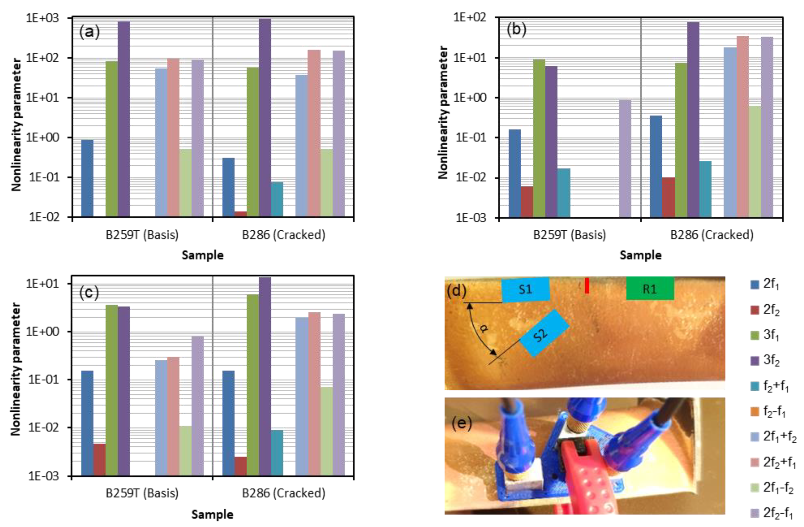
Results and Discussion
Figure 33 shows the nonlinear parameter measurements on the trailing edges of the turbine blades. The left sides of the figure illustrate the results of the undamaged blade (B259T). The sensors were positioned on the opposite side of the cooling air outlet slots, where a continuous surface is given.
In Figure 33a, an important indicator is that 2f2 occurs only in the damaged sample. The parameter values of 2f2+f1 and 2f2−f1 show a significant increase in the damaged sample.
At a sensor angle of α = 60° (shown in Figure 33b), the harmonic frequencies 2f1−f2, 2f2+f1, and 2f1+f2 were regressed exclusively on the measurements on the damaged sample. With 2f1, 2f2, 3f2, and f2+f1, an increase of the parameters is measurable compared to the reference sample.
At an angle of α = 90° (Figure 33c), the frequency f2−f1 was not measured at both samples. Most other higher harmonic frequencies also indicate an increase in the parameter values. Those dependent on one frequency like 2f1, 3f1, and 3f2 but also the combination harmonics of two frequencies, f2±f1, 2f1±f2, and 2f2±f1, show a clear increase in their parameter values.
All three combinations of angles were able to clearly identify the crack in the turbine blade. However, the sensor arrangement at 60° and 90° showed clearer changes in the nonlinear parameter values.
5. Conclusions
The aim of this study was the development of a frequency modulated nonlinear ultrasonic technique for the detection of cracks in turbine blades. New global nonlinearity parameters were developed to determine a correlation between the crack length and the measured nonlinear features. Their existence has been proven numerically and experimentally. A simple method for adding up the amplitude amounts of the fundamental amplitudes and harmonic amplitudes are used for the crack prediction. The behavior of the fundamental frequencies is also a good indicator for crack detection and crack size estimation. Therefore, the linear parameters and have been proposed.
New sample types made of metal plates, produced with a welding process and SLM technology, were used. Different sensor angle combinations were compared, and in addition to the plate samples, tests were carried out with turbine guide vanes and rotor blades. The results show a clear trend of changing nonlinear parameters as a function of crack size and sensor angles. In all measurements, a dependence of the sensor position to the defect was observed.
It was shown that each crack behaves individually during the ultrasound measurements, since the highest nonlinearities were often found in small- and medium-sized defects. Nevertheless, it became clear that the interactions from the various harmonic frequencies also offer very good additions or alternatives to the already existing measurements and evaluation variants.
This study demonstrates an efficient way to determine the initial loss of structural integrity of these complex components.
Author Contributions
M.M. designed the project and F.M. the experiments. F.M. performed the experiments and wrote the paper with support from M.M. All authors contributed to the general discussion. All authors have read and agreed to the published version of the manuscript.
Funding
This research was funded by the European Commission through the project TurboReflex, grant agreement no. 764545.
Acknowledgments
Thanks to the MAN Energy Solutions SE for their support.
Conflicts of Interest
The authors declare no conflict of interest.
References
- Li, Z.L.; Achenbach, J.D. Reflection and Transmission of Rayleigh Surface Waves by a Material Interphase. J. Appl. Mech. 1991, 58, 688. [Google Scholar] [CrossRef]
- Achenbach, J.D.; Lin, W.; Keer, L.M. Mathematical Modelling of Ultrasonic Wave Scattering by sub-Surface Cracks. Ultrasonics 1986, 24, 207–215. [Google Scholar] [CrossRef]
- Angel, Y.C.; Achenbach, J.D. Reflection and Transmission of Obliquely Incident Rayleigh Waves by a Surface-Breaking Crack. Acoust. Soc. Am. 1983, 74, S87. [Google Scholar] [CrossRef]
- Hikata, A.; Chick, B.B.; Elbaum, C. Dislocation Contribution to the Second Harmonic Generation of Ultrasonic Waves. J. Appl. Phys. 1965, 36, 229–236. [Google Scholar] [CrossRef]
- Cantrell, J.H.; Yost, W.T. Nonlinear Ultrasonic Characterization of Fatigue Microstructures. Int. J. Fatigue 2001, 23, 487–490. [Google Scholar] [CrossRef]
- Mitra, M.; Gopalakrishnan, S. Guided Wave Based Structural Health Monitoring: A Review. Smart Mater. Struct. 2016, 25, 53001. [Google Scholar] [CrossRef]
- Cho, H.; Lissenden, C.J. Structural Health Monitoring of Fatigue Crack Growth in Plate Structures with Ultrasonic Guided Waves. Struct. Health Monit. 2012, 11, 393–404. [Google Scholar] [CrossRef]
- Chan, H.; Masserey, B.; Fromme, P. High Frequency Guided Ultrasonic Waves for Hidden Fatigue Crack Growth Monitoring in multi-Layer Model Aerospace Structures. Smart Mater. Struct. 2015, 24, 25037. [Google Scholar] [CrossRef] [Green Version]
- Masserey, B.; Fromme, P. Analysis of High Frequency Guided Wave Scattering at a Fastener Hole with a View to Fatigue Crack Detection. Ultrasonics 2017, 76, 78–86. [Google Scholar] [CrossRef]
- Masserey, B.; Fromme, P. Fatigue Crack Growth Monitoring Using High-Frequency Guided Waves. Struct. Health Monit. 2013, 12, 484–493. [Google Scholar] [CrossRef] [Green Version]
- Masserey, B.; Fromme, P. Noncontact monitoring of fatigue crack growth using high frequency guided waves. In Proceedings of the SPIE 9061, Sensors and Smart Structures Technologies for Civil, Mechanical, and Aerospace Systems 2014, Bellingham, WA, USA, 8 March 2014. [Google Scholar]
- Broda, D.; Staszewski, W.J.; Martowicz, A.; Uhl, T.; Silberschmidt, V.V. Modelling of Nonlinear Crack—Wave Interactions for Damage Detection Based on Ultrasound—A Review. J. Sound Vib. 2014, 333, 1097–1118. [Google Scholar] [CrossRef]
- Guan, L.; Zou, M.; Wan, X.; Li, Y. Nonlinear Lamb Wave Micro-Crack Direction Identification in Plates with Mixed-Frequency Technique. Appl. Sci. 2020, 10, 2135. [Google Scholar] [CrossRef] [Green Version]
- Lim, H.J.; Sohn, H. Online Fatigue Crack Prognosis Using Nonlinear Ultrasonic Modulation. Struct. Health Monit. 2019, 18, 1889–1902. [Google Scholar] [CrossRef]
- Mihara, T.; Konishi, G.; Miura, Y.; Ishida, H. Accurate sizing of closed crack using nonlinear ultrasound of space with high voltage transformer pulser technique. In Proceedings of the American Institute of Physics Conference, Baltimore, MD, USA, 21–26 July 2013; AIP Publishing LLC: Melville, NY, USA, 2014; pp. 727–732. [Google Scholar]
- Moll, J.; Kexel, C.; Pötzsch, S.; Rennoch, M.; Herrmann, A.S. Temperature Affected Guided Wave Propagation in a Composite Plate Complementing the Open Guided Waves Platform. Sci. Data 2019, 6, 191. [Google Scholar] [CrossRef] [PubMed]
- Pan, Q.; Pan, R.; Shao, C.; Chang, M.; Xu, X. Research Review of Principles and Methods for Ultrasonic Measurement of Axial Stress in Bolts. Chin. J. Mech. Eng. 2020, 33, 1–16. [Google Scholar] [CrossRef] [Green Version]
- Jhang, K.-Y.; Kim, K.-C. Evaluation of Material Degradation Using Nonlinear Acoustic Effect. Ultrasonics 1999, 37, 39–44. [Google Scholar] [CrossRef]
- Frouin, J.; Sathish, S.; Matikas, T.E.; Na, J.K. Ultrasonic Linear and Nonlinear Behavior of Fatigued Ti–6Al–4V. J. Mater. Res. 1999, 14, 1295–1298. [Google Scholar] [CrossRef]
- Rothenfusser, M.; Mayr, M.; Baumann, J. Acoustic Nonlinearities in Adhesive Joints. Ultrasonics 2000, 38, 322–326. [Google Scholar] [CrossRef]
- Yost, W.T. Nonlinear ultrasonic pulsed measurements and applications to metal processing and fatigue. In Proceedings of the 27th Annual Review of Progress in Quantitative Nondestructive Evaluation, Ames, IA, USA, 16–20 July 2000; AIP: Melville, NY, USA, 2000; pp. 1268–1275. [Google Scholar]
- Boccardi, S.; Callá, D.B.; Ciampa, F.; Meo, M. Nonlinear Elastic multi-Path Reciprocal Method for Damage Localisation in Composite Materials. Ultrasonics 2018, 82, 239–245. [Google Scholar] [CrossRef] [Green Version]
- Jeong, H.; Nahm, S.-H.; Jhang, K.-Y.; Nam, Y.-H. A Nondestructive Method for Estimation of the Fracture Toughness of CrMoV Rotor Steels Based on Ultrasonic Nonlinearity. Ultrasonics 2003, 41, 543–549. [Google Scholar] [CrossRef]
- Ostrovsky, L.A.; Johnson, P.A. Dynamic nonlinear elasticity in geomaterials. La Rivista del Nuovo Cimento 2001, 24, 1–46. [Google Scholar]
- Straka, L.; Yagodzinskyy, Y.; Landa, M.; Hänninen, H. Detection of Structural Damage of Aluminum Alloy 6082 Using Elastic Wave Modulation Spectroscopy. NDT & E Int. 2008, 41, 554–563. [Google Scholar]
- Malfense Fierro, G.P.; Meo, M. Residual Fatigue Life Estimation Using a Nonlinear Ultrasound Modulation Method. Smart Mater. Struct. 2015, 24, 25040. [Google Scholar] [CrossRef]
- Malfense Fierro, G.P.; Meo, M. Nonlinear Imaging (NIM) of Flaws in a Complex Composite Stiffened Panel Using a Constructive Nonlinear Array (CNA) Technique. Ultrasonics 2017, 74, 30–47. [Google Scholar] [CrossRef] [PubMed] [Green Version]
- Malfense Fierro, G.P. Development of Nonlinear Ultrasound Techniques for Multidisciplinary Engineering Applications. Ph.D. Thesis, University of Bath, Bath, UK, 2014. [Google Scholar]
- Jingpin, J.; Xiangji, M.; Cunfu, H.; Bin, W. Nonlinear Lamb Wave-Mixing Technique for micro-Crack Detection in Plates. NDT & E Int. 2017, 85, 63–71. [Google Scholar]
- Amura, M.; Meo, M.; Amerini, F. Baseline-free Estimation of Residual Fatigue Life Using a Third Order Acoustic Nonlinear Parameter. Acoust. Soc. Am. 2011, 130, 1829–1837. [Google Scholar] [CrossRef] [Green Version]
- TenCate, J.A.; van den Abeele, K.E.A.; Shankland, T.J.; Johnson, P.A. Laboratory Study of Linear and Nonlinear Elastic Pulse Propagation in Sandstone. J. Acoust. Soc. Am. 1996, 100, 1383–1391. [Google Scholar] [CrossRef] [Green Version]
- Bermes, C.; Kim, J.-Y.; Qu, J.; Jacobs, L.J. Nonlinear Lamb Waves for the Detection of Material Nonlinearity. Mech. Syst. Signal Process. 2008, 22, 638–646. [Google Scholar] [CrossRef]
- Herrmann, J.; Kim, J.-Y.; Jacobs, L.J.; Qu, J.; Littles, J.W.; Savage, M.F. Assessment of Material Damage in a Nickel-Base Superalloy Using Nonlinear Rayleigh Surface Waves. J. Appl. Phys. 2006, 99, 124913. [Google Scholar] [CrossRef]
- Markovic, N.; Stojic, D.; Cvetkovic, R.; Radojicic, V.; Conic, S. Numerical Modeling of Ultrasonic Wave Propagation-by Using of Explicit FEM in ABAQUS. Facta Univ. Ser. Archit. Civ. Eng. 2018, 16, 135–147. [Google Scholar] [CrossRef]
- Schwarz, C.; Werner, E.; Dirschmid, H.J. 1D Wave Propagation in a Rod: Analytic Treatment for non-Trivial Boundary Conditions. Proc. Appl. Math. Mech. 2010, 10, 525–526. [Google Scholar] [CrossRef]
- Cui, Z.; Huang, Y. Discussion on Acoustic Databases in LS-DYNA. 2017. Available online: http://www.lstc.com/sites/default/files/marketing/new_features/12_Acoustic_Databases_ZheCui_2017_01.pdf (accessed on 8 March 2020).
- Maraghechi, B.; Hasani, M.H.; Kolios, M.C.; Tavakkoli, J. Temperature Dependence of Acoustic Harmonics Generated by Nonlinear Ultrasound Wave Propagation in Water at Various Frequencies. J. Acoust. Soc. Am. 2016, 139, 2475. [Google Scholar] [CrossRef] [PubMed] [Green Version]
- Song, B.; Zhao, X.; Li, S.; Han, C.; Wei, Q.; Wen, S.; Liu, J.; Shi, Y. Differences in Microstructure and Properties between Selective Laser Melting and Traditional Manufacturing for Fabrication of Metal Parts: A Review. Front. Mech. Eng. 2015, 10, 111–125. [Google Scholar] [CrossRef]
Figure 1.
Experiments (a) Specimen—overview; (b) Experimental setup—principle.

Figure 2.
Nonlinearity parameter: (a) f1 = 3 MHz, f2 = 5 MHz; (b) f1 = 4 MHz, f2 = 5 MHz.
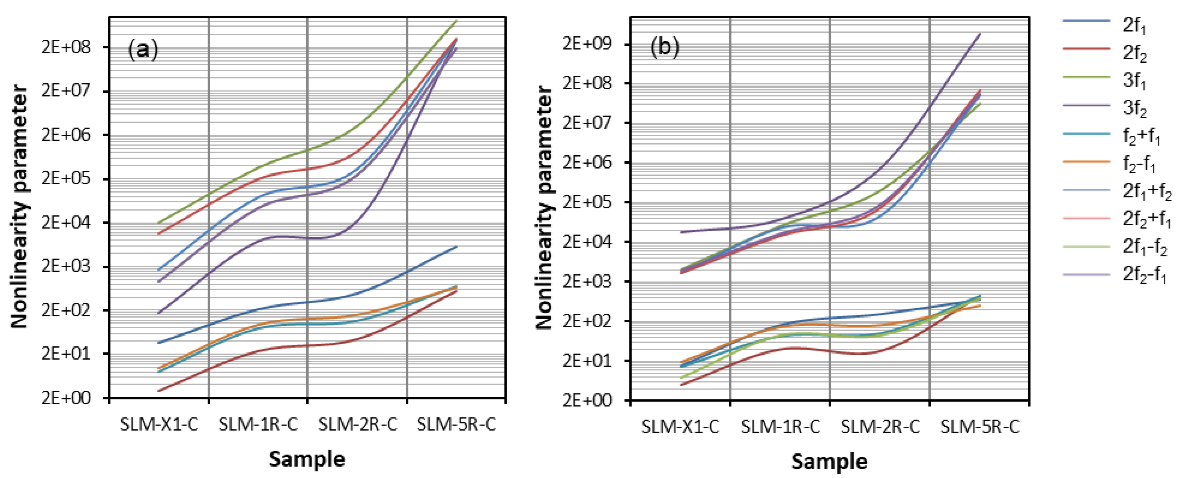
Figure 3.
Quasi-one-dimensional LS-DYNA model.
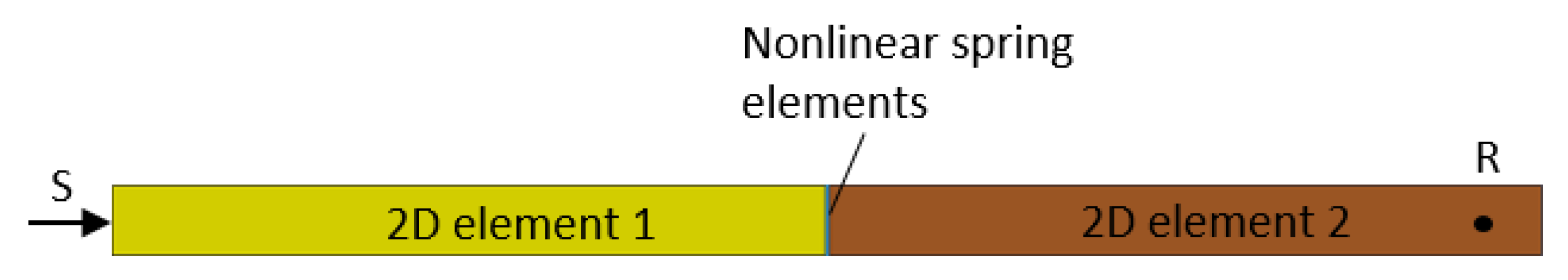
Figure 4.
Quasi-one-dimensional frequency spectrum, LS-DYNA simulation with excitation frequency f = 5 MHz.
Figure 4.
Quasi-one-dimensional frequency spectrum, LS-DYNA simulation with excitation frequency f = 5 MHz.
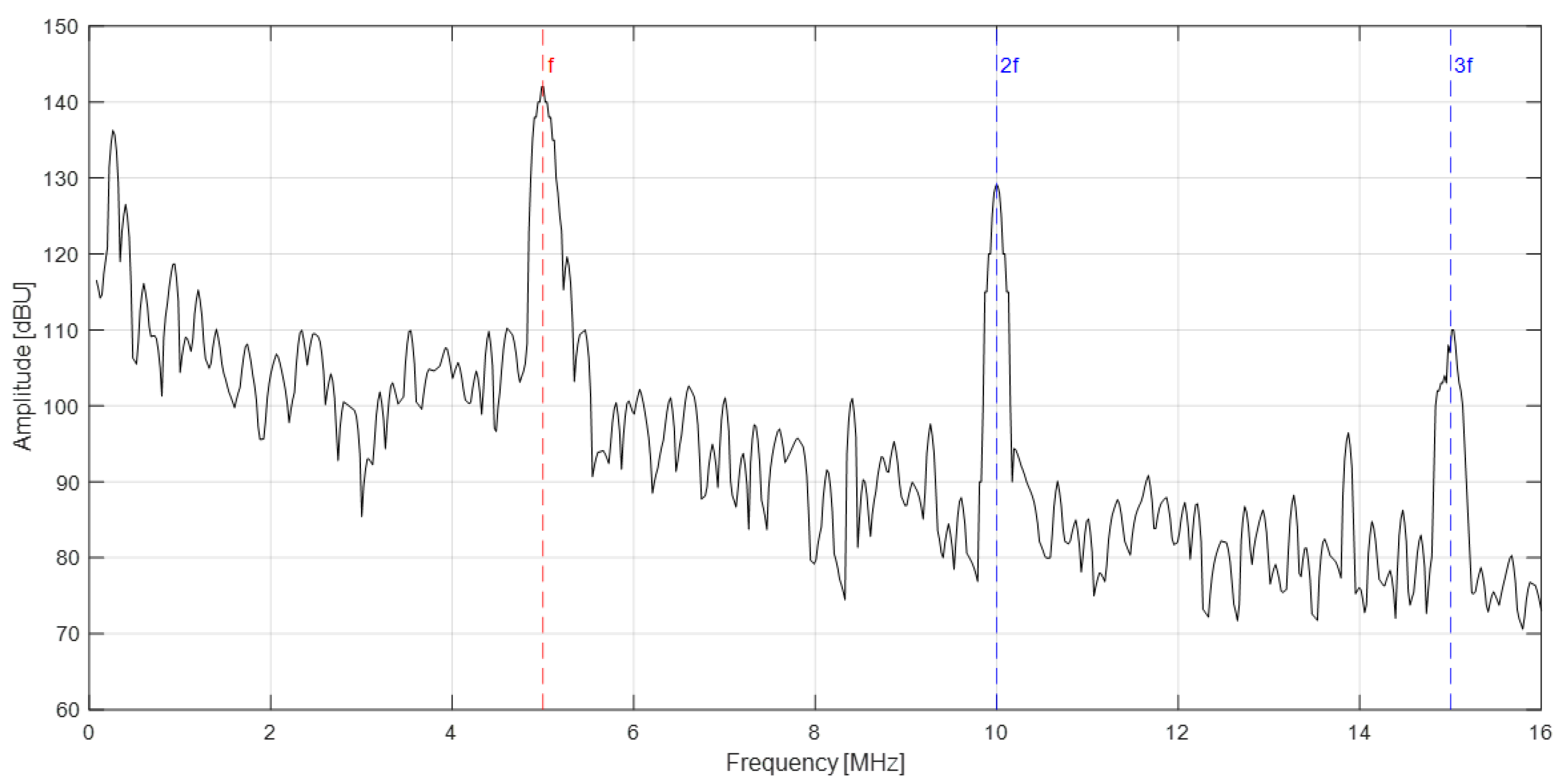
Figure 5.
LS-DYNA model.
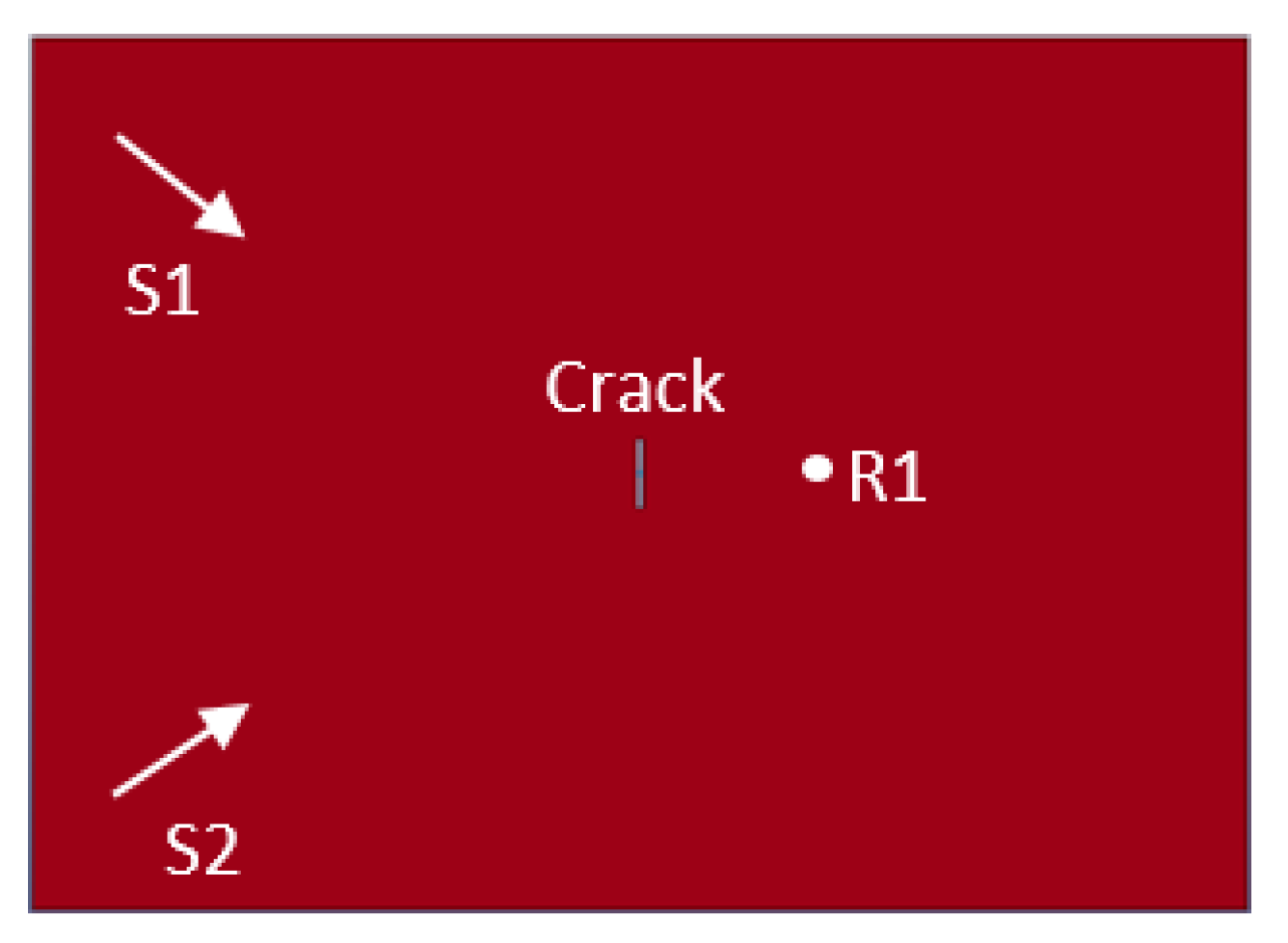
Figure 6.
Wave propagation: (a) t = 2.4 × 10⁻⁹ s; (b) t = 6.8 × 10⁻⁹ s; (c) t = 1.2 × 10⁻⁸ s; (d) t = 3.6 × 10⁻⁸ s; (e) t = 5.3 × 10⁻⁸ s; (f) t = 1.1 × −7 s.
Figure 6.
Wave propagation: (a) t = 2.4 × 10⁻⁹ s; (b) t = 6.8 × 10⁻⁹ s; (c) t = 1.2 × 10⁻⁸ s; (d) t = 3.6 × 10⁻⁸ s; (e) t = 5.3 × 10⁻⁸ s; (f) t = 1.1 × −7 s.
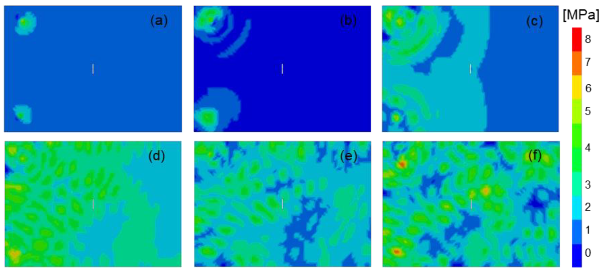
Figure 7.
Frequency spectrum, LS-DYNA simulation with excitation frequencies f1 = 3 MHz and f2 = 5 MHz.
Figure 7.
Frequency spectrum, LS-DYNA simulation with excitation frequencies f1 = 3 MHz and f2 = 5 MHz.
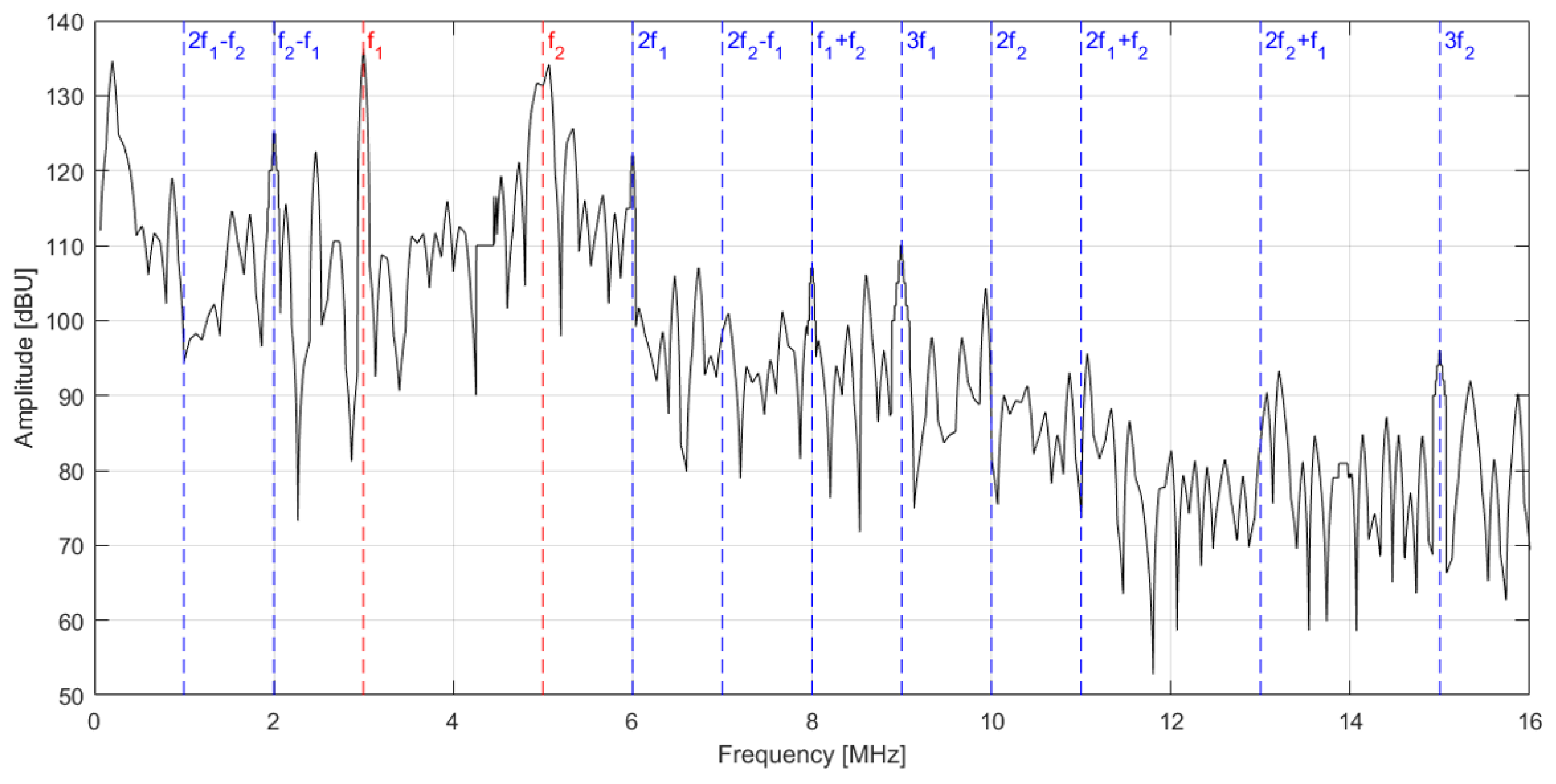
Figure 8.
Frequency spectrum, LS-DYNA simulation with excitation frequencies f1 = 4 MHz and f2 = 5 MHz.
Figure 8.
Frequency spectrum, LS-DYNA simulation with excitation frequencies f1 = 4 MHz and f2 = 5 MHz.
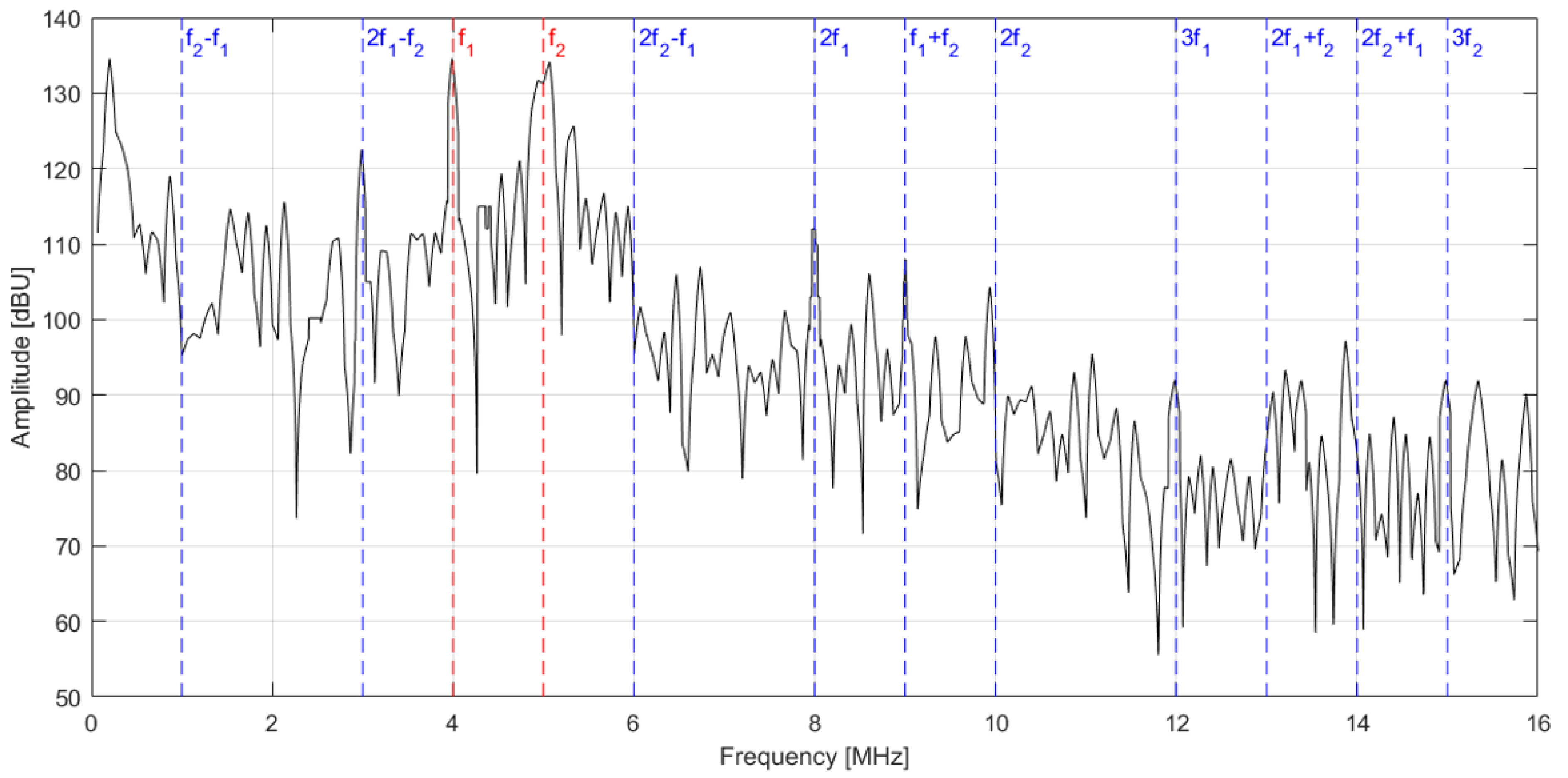
Figure 9.
Experimental setup.

Figure 10.
Damage detection methodology.
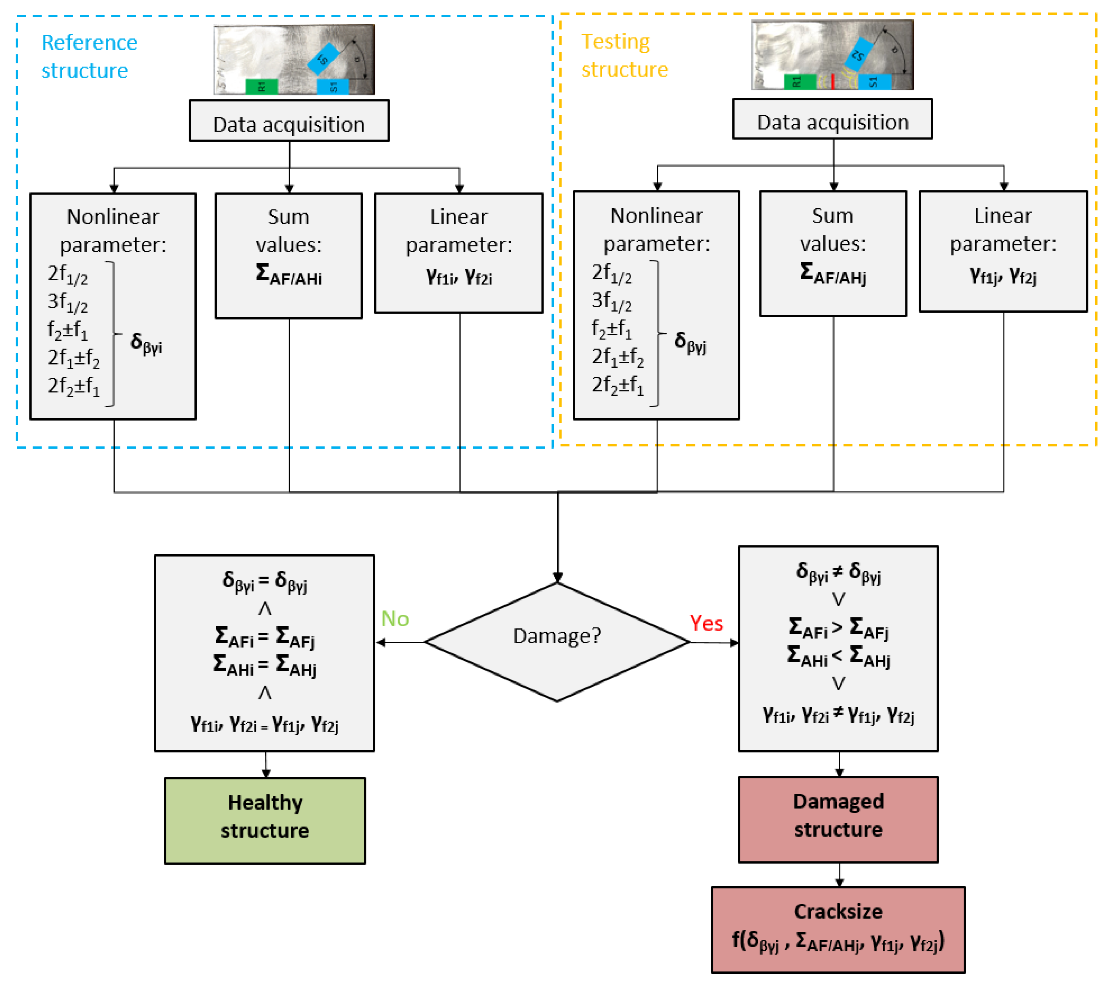
Figure 11.
Comparison of frequency spectrum: f1 = 3 MHz, f2 = 5 MHz, α = 60°.
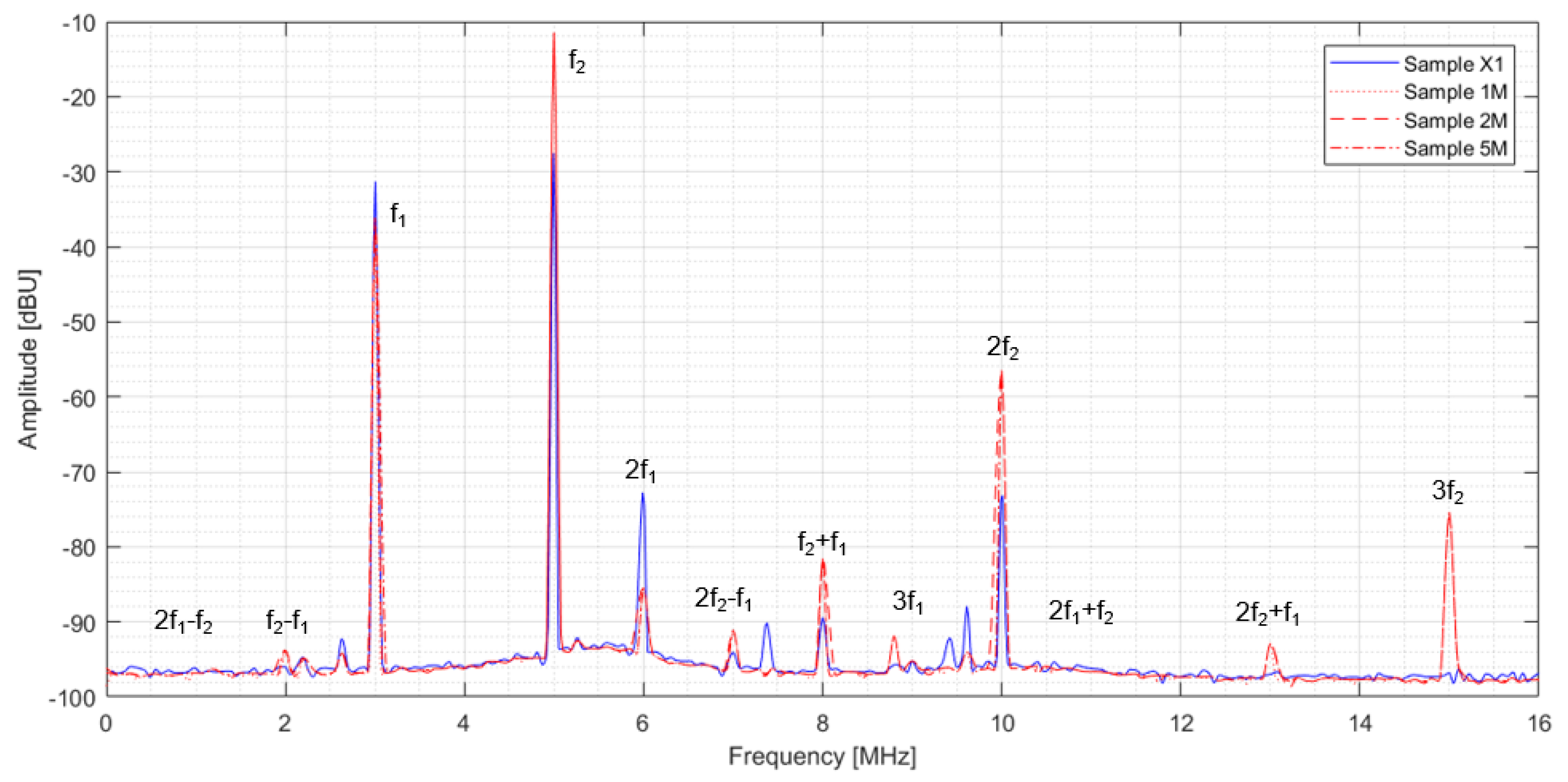
Figure 12.
Comparison of frequency spectrum: f1 = 4 MHz, f2 = 5 MHz, α = 60°.
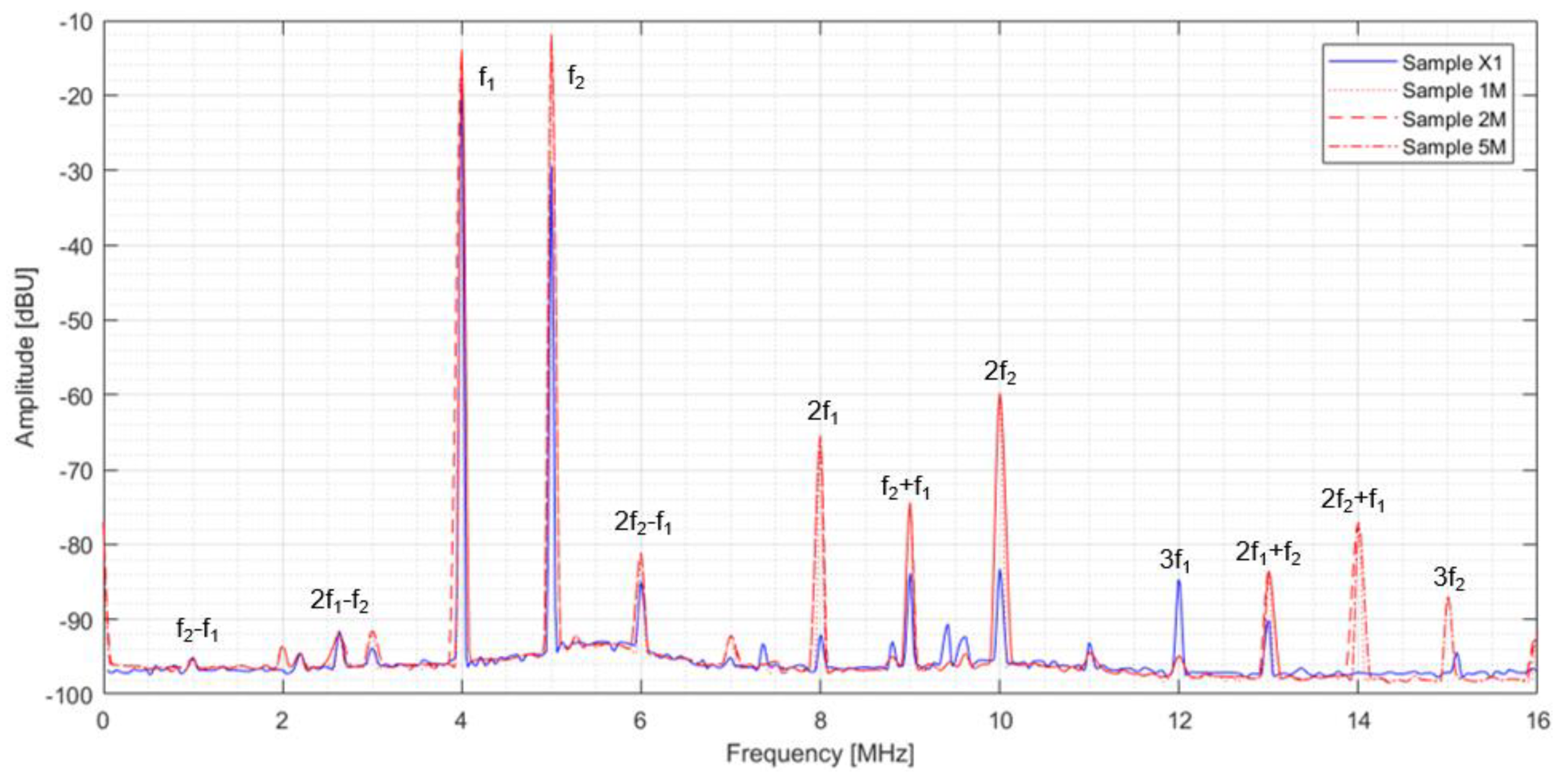
Figure 13.
Measuring principle—sample with central defect.
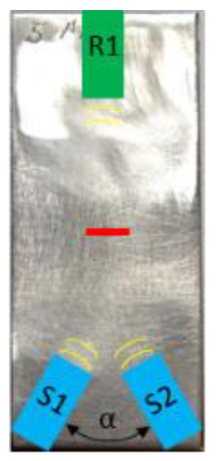
Figure 14.
Nonlinearity parameter: (a) f1 = 3 MHz, f2 = 5 MHz, α = 50°; (b) f1 = 4 MHz, f2 = 5 MHz, α = 50°.
Figure 14.
Nonlinearity parameter: (a) f1 = 3 MHz, f2 = 5 MHz, α = 50°; (b) f1 = 4 MHz, f2 = 5 MHz, α = 50°.
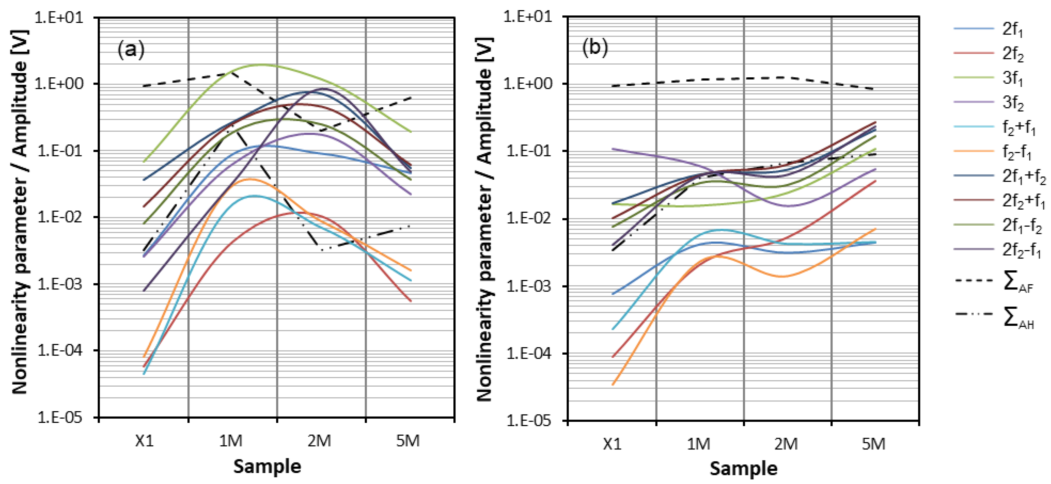
Figure 15.
Nonlinearity parameter: (a) f1 = 3 MHz, f2 = 5 MHz, α = 60°; (b) f1 = 4 MHz, f2 = 5 MHz, α = 60°.
Figure 15.
Nonlinearity parameter: (a) f1 = 3 MHz, f2 = 5 MHz, α = 60°; (b) f1 = 4 MHz, f2 = 5 MHz, α = 60°.
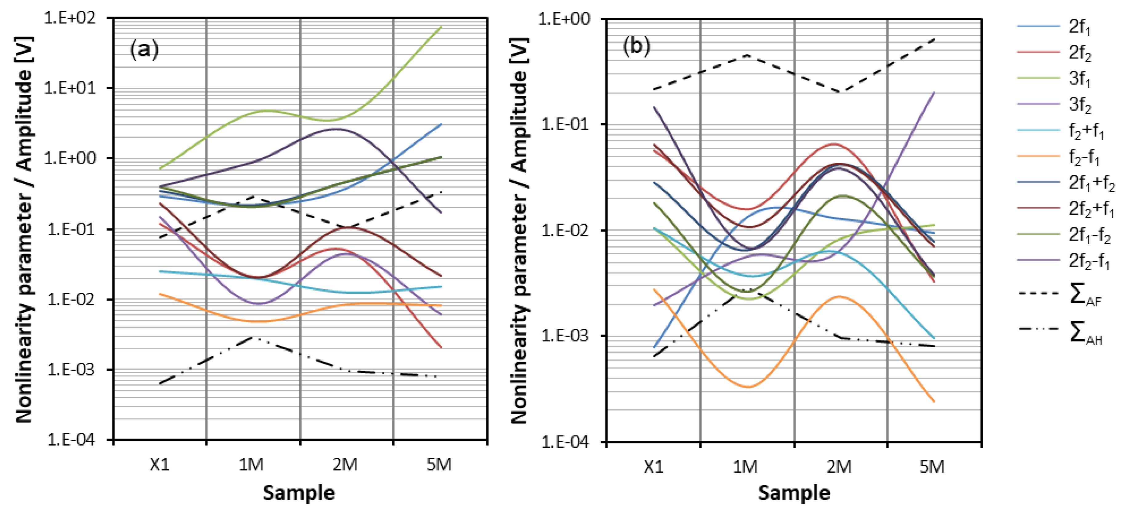
Figure 16.
Nonlinearity parameter: (a) f1 = 3 MHz, f2 = 5 MHz, α = 90°; (b) f1 = 4 MHz, f2 = 5 MHz, α = 90°.
Figure 16.
Nonlinearity parameter: (a) f1 = 3 MHz, f2 = 5 MHz, α = 90°; (b) f1 = 4 MHz, f2 = 5 MHz, α = 90°.
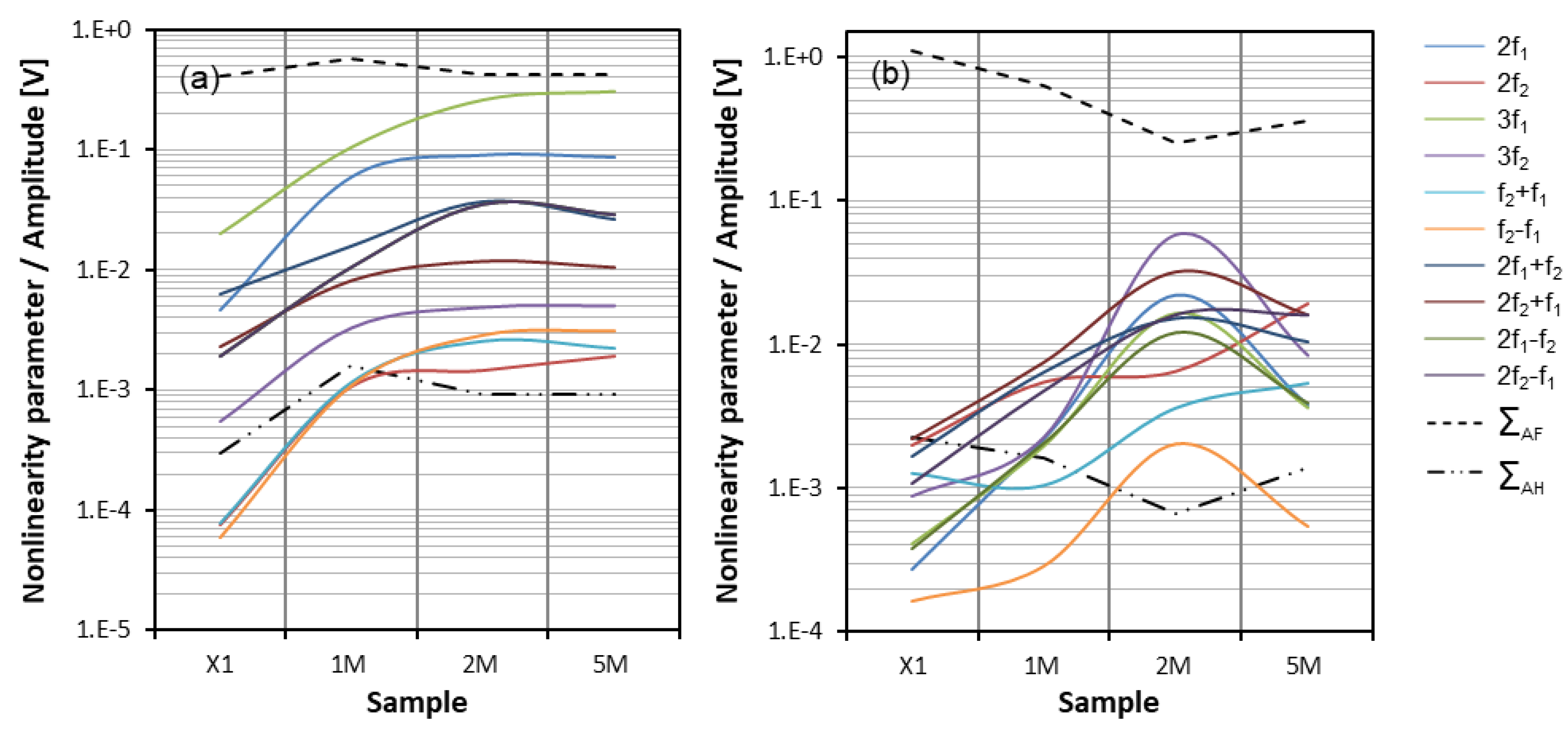
Figure 17.
Comparison of and parameters: (a) α = 50°; (b) α = 60°; (c) α = 90°.
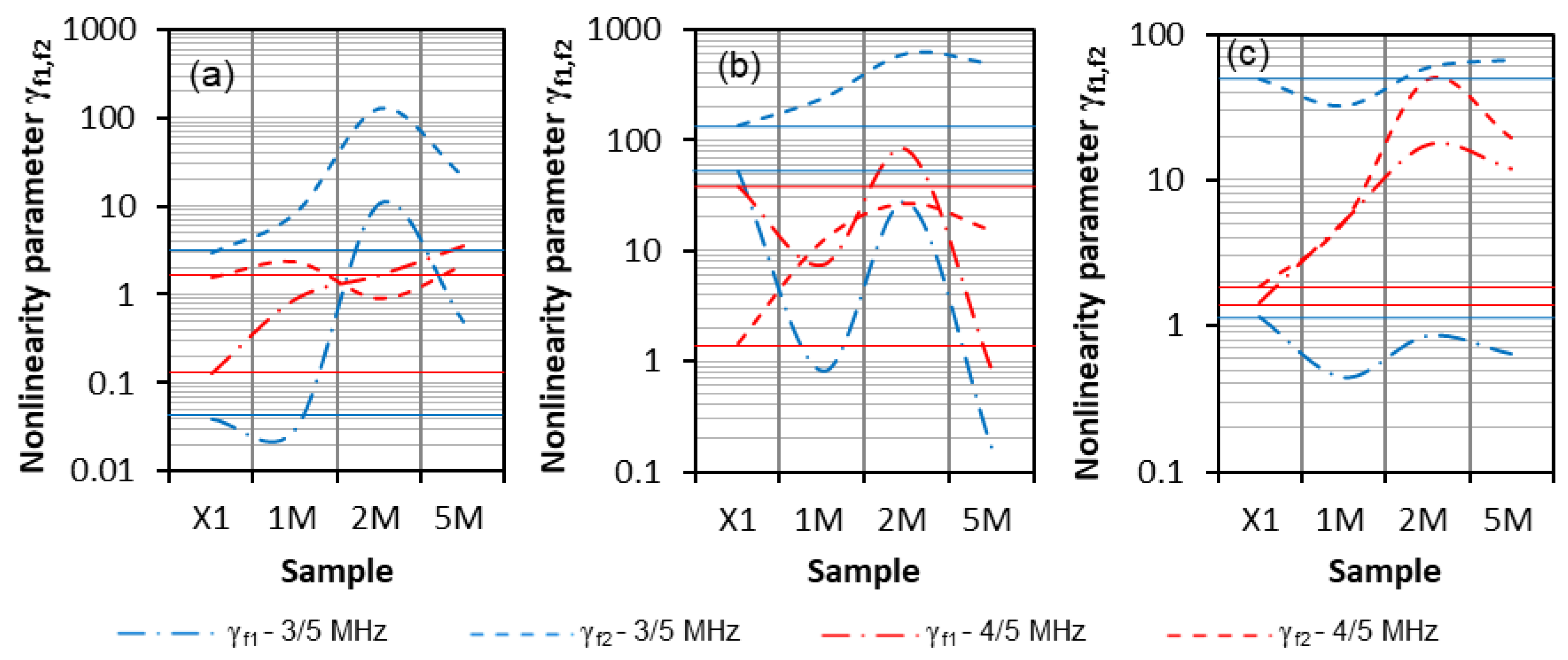
Figure 18.
Measuring principle—sample with lateral defect.
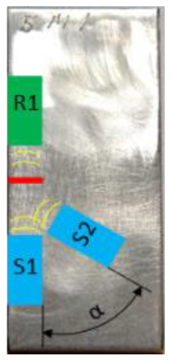
Figure 19.
Nonlinearity parameter: (a) f1 = 3 MHz, f2 = 5 MHz, α = 45°; (b) f1 = 4 MHz, f2 = 5 MHz, α = 45°.
Figure 19.
Nonlinearity parameter: (a) f1 = 3 MHz, f2 = 5 MHz, α = 45°; (b) f1 = 4 MHz, f2 = 5 MHz, α = 45°.
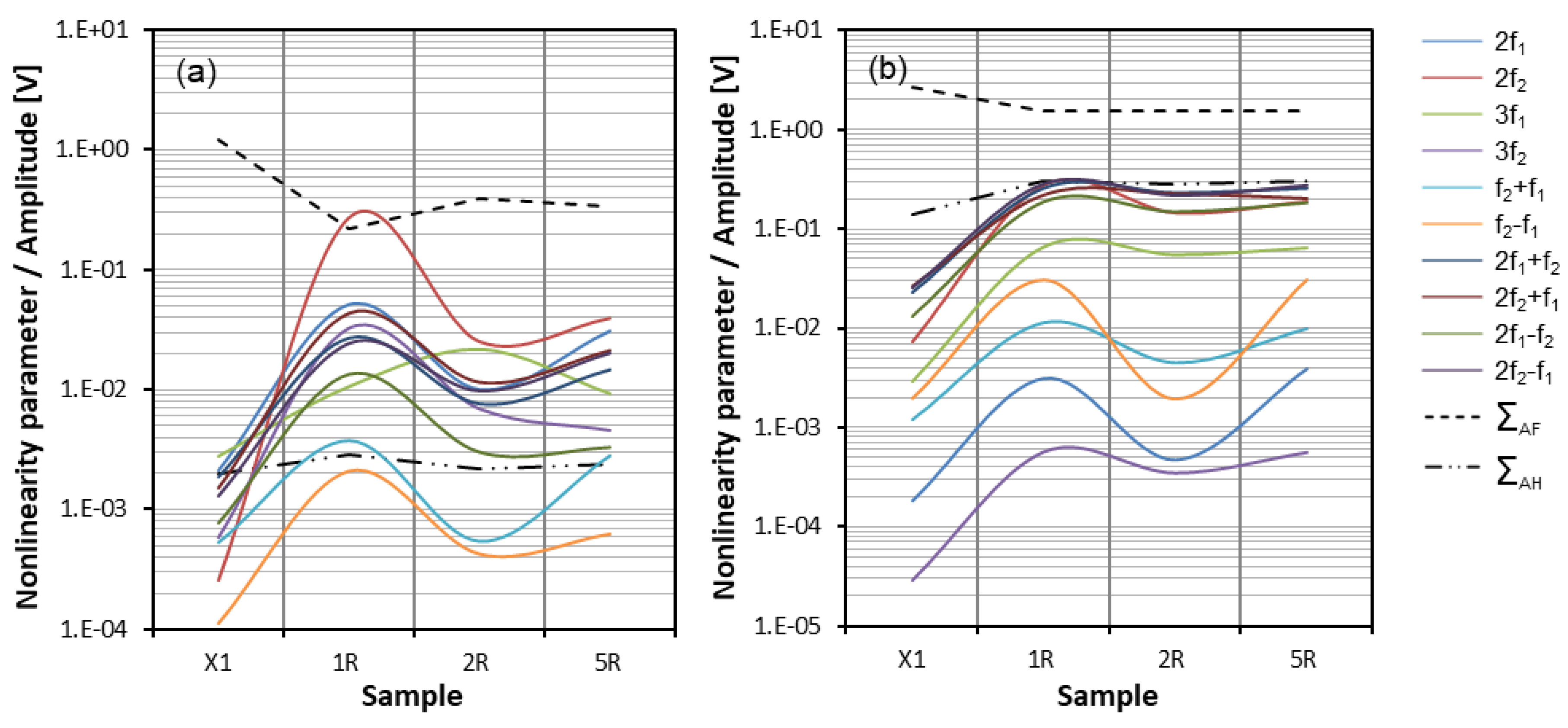
Figure 20.
Nonlinearity parameter: (a) f1 = 3 MHz, f2 = 5 MHz, α = 60°; (b) f1 = 4 MHz, f2 = 5 MHz, α = 60°.
Figure 20.
Nonlinearity parameter: (a) f1 = 3 MHz, f2 = 5 MHz, α = 60°; (b) f1 = 4 MHz, f2 = 5 MHz, α = 60°.
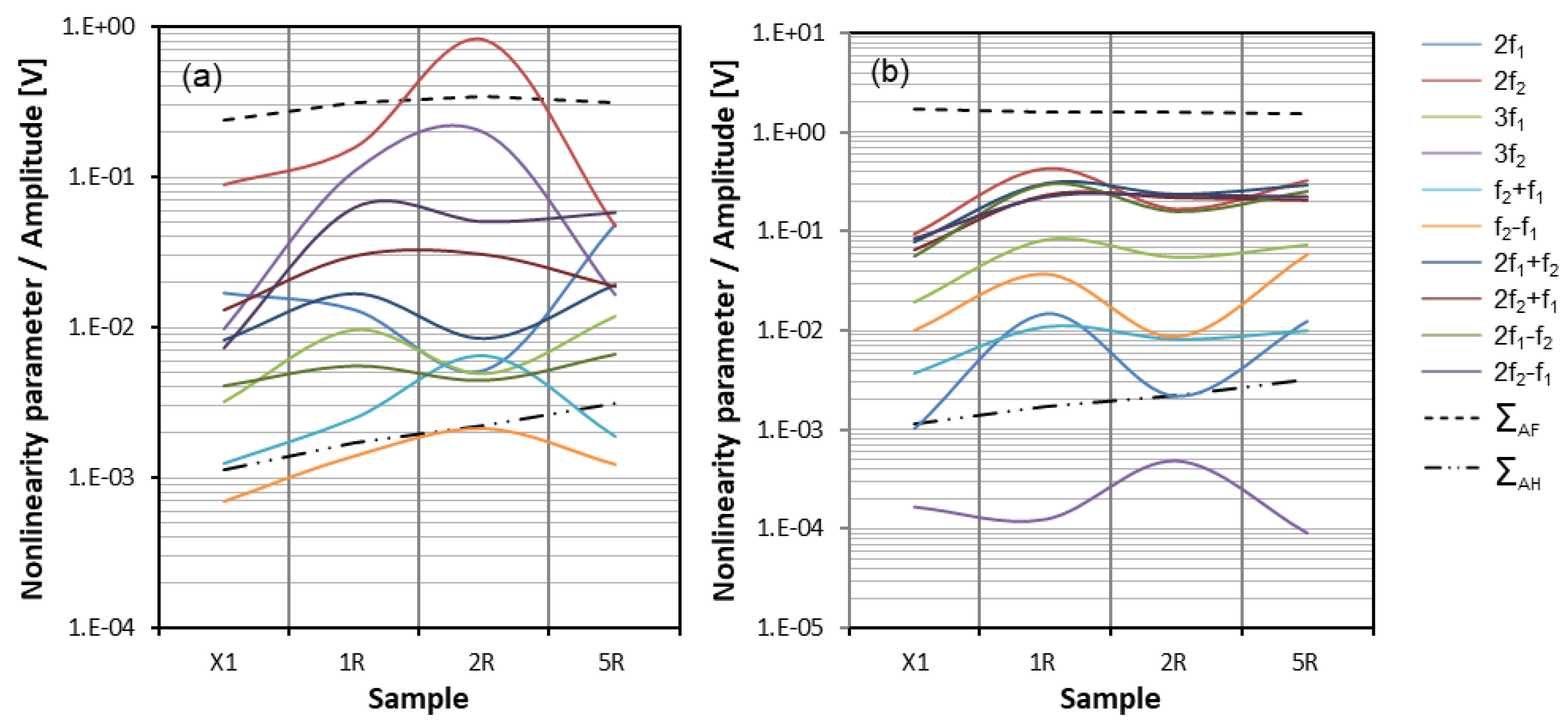
Figure 21.
Nonlinearity parameter: (a) f1 = 3 MHz, f2 = 5 MHz, α = 90°; (b) f1 = 4 MHz, f2 = 5 MHz, α = 90°.
Figure 21.
Nonlinearity parameter: (a) f1 = 3 MHz, f2 = 5 MHz, α = 90°; (b) f1 = 4 MHz, f2 = 5 MHz, α = 90°.

Figure 22.
Comparison of and parameters: (a) α = 45°; (b) α = 60°; (c) α = 90°.
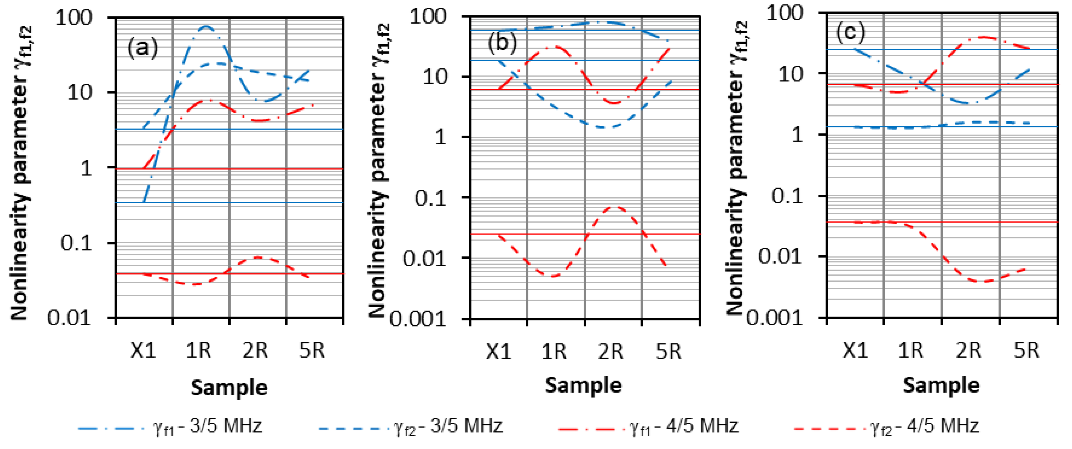
Figure 23.
SLM samples: (a) Reference sample SLM-X1; (b) Sample SLM-1R; (c) Sample SLM-2R; (d) Sample SLM-5R.
Figure 23.
SLM samples: (a) Reference sample SLM-X1; (b) Sample SLM-1R; (c) Sample SLM-2R; (d) Sample SLM-5R.
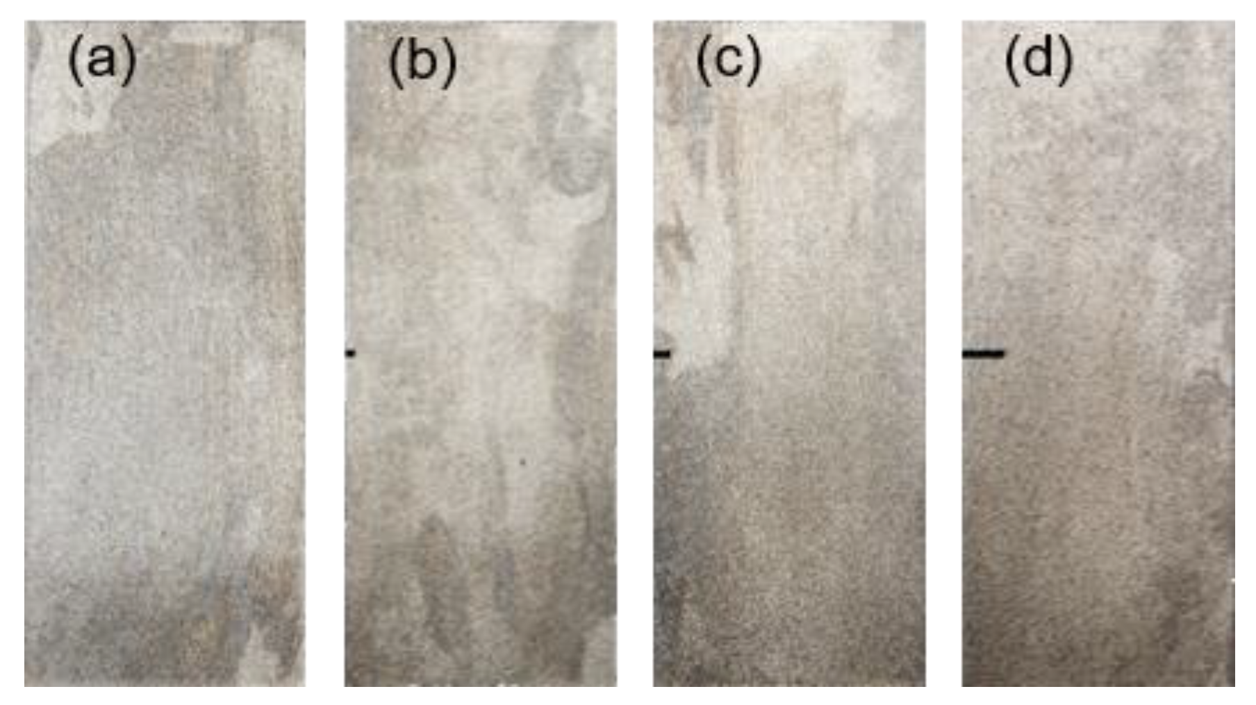
Figure 24.
Nonlinearity parameter: (a) f1 = 3 MHz, f2 = 5 MHz, α = 45°; (b) f1 = 4 MHz, f2 = 5 MHz, α = 45°.
Figure 24.
Nonlinearity parameter: (a) f1 = 3 MHz, f2 = 5 MHz, α = 45°; (b) f1 = 4 MHz, f2 = 5 MHz, α = 45°.
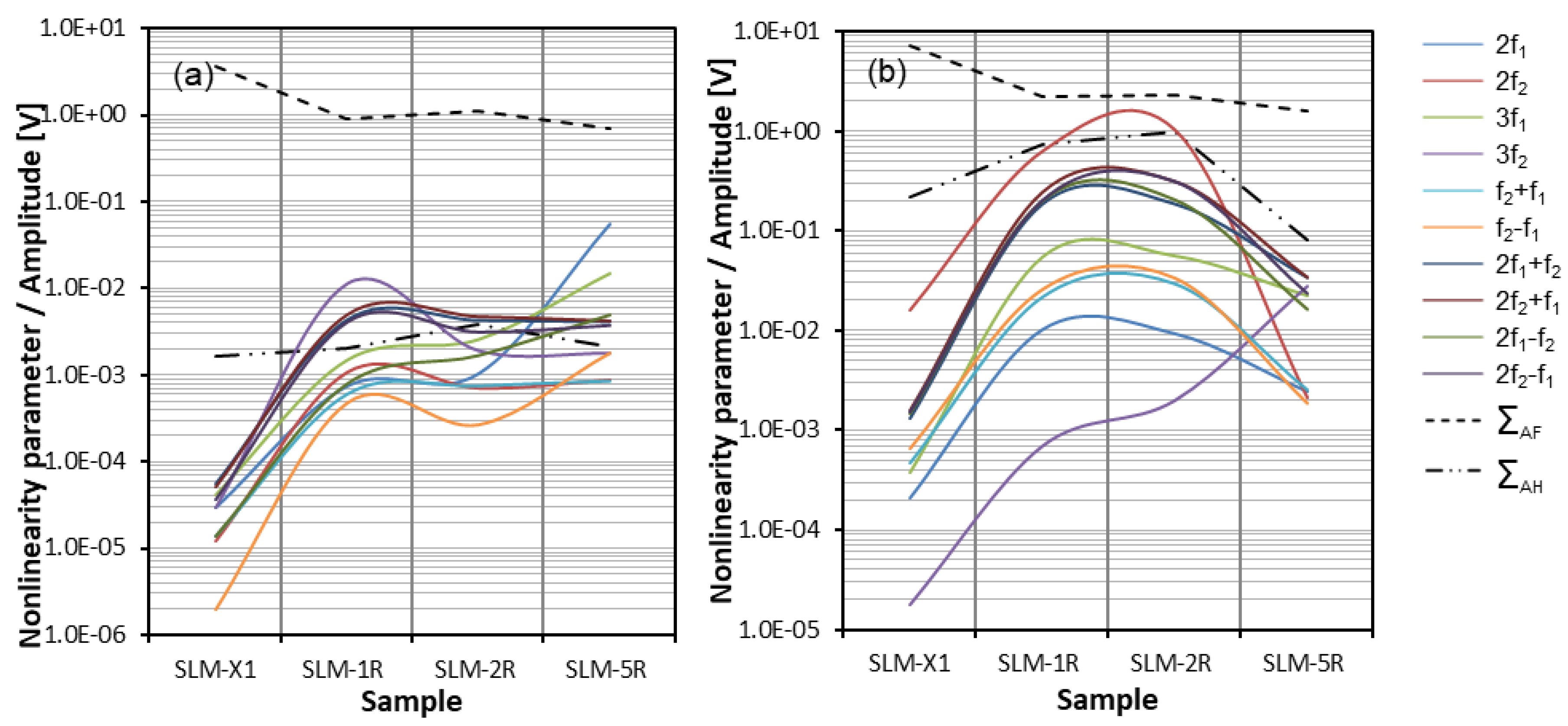
Figure 25.
Nonlinearity parameter: (a) f1 = 3 MHz, f2 = 5 MHz, α = 60°; (b) f1 = 4 MHz, f2 = 5 MHz, α = 60°.
Figure 25.
Nonlinearity parameter: (a) f1 = 3 MHz, f2 = 5 MHz, α = 60°; (b) f1 = 4 MHz, f2 = 5 MHz, α = 60°.
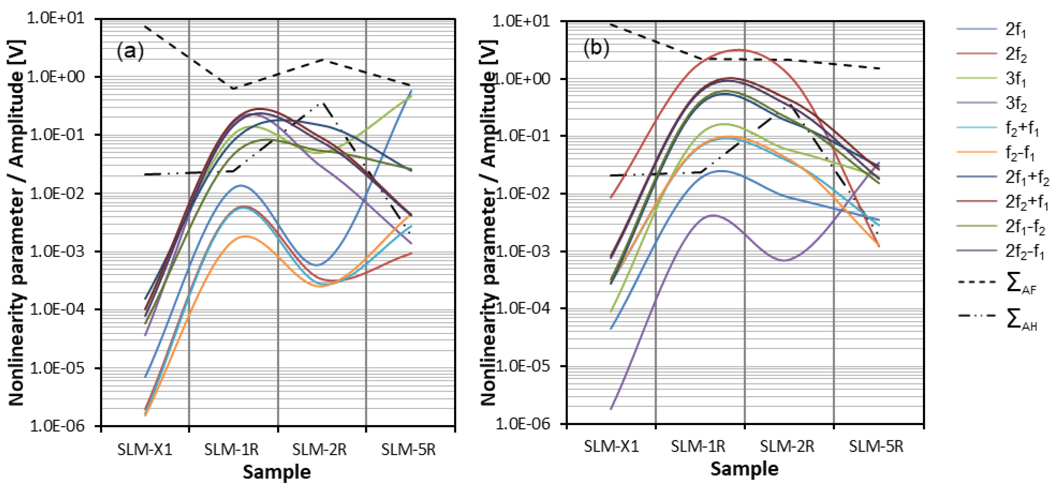
Figure 26.
Nonlinearity parameter: (a) f1 = 3 MHz, f2 = 5 MHz, α = 90°; (b) f1 = 4 MHz, f2 = 5 MHz, α = 90°.
Figure 26.
Nonlinearity parameter: (a) f1 = 3 MHz, f2 = 5 MHz, α = 90°; (b) f1 = 4 MHz, f2 = 5 MHz, α = 90°.

Figure 27.
Comparison of and parameters: (a) α = 45°; (b) α = 60°; (c) α = 90°.
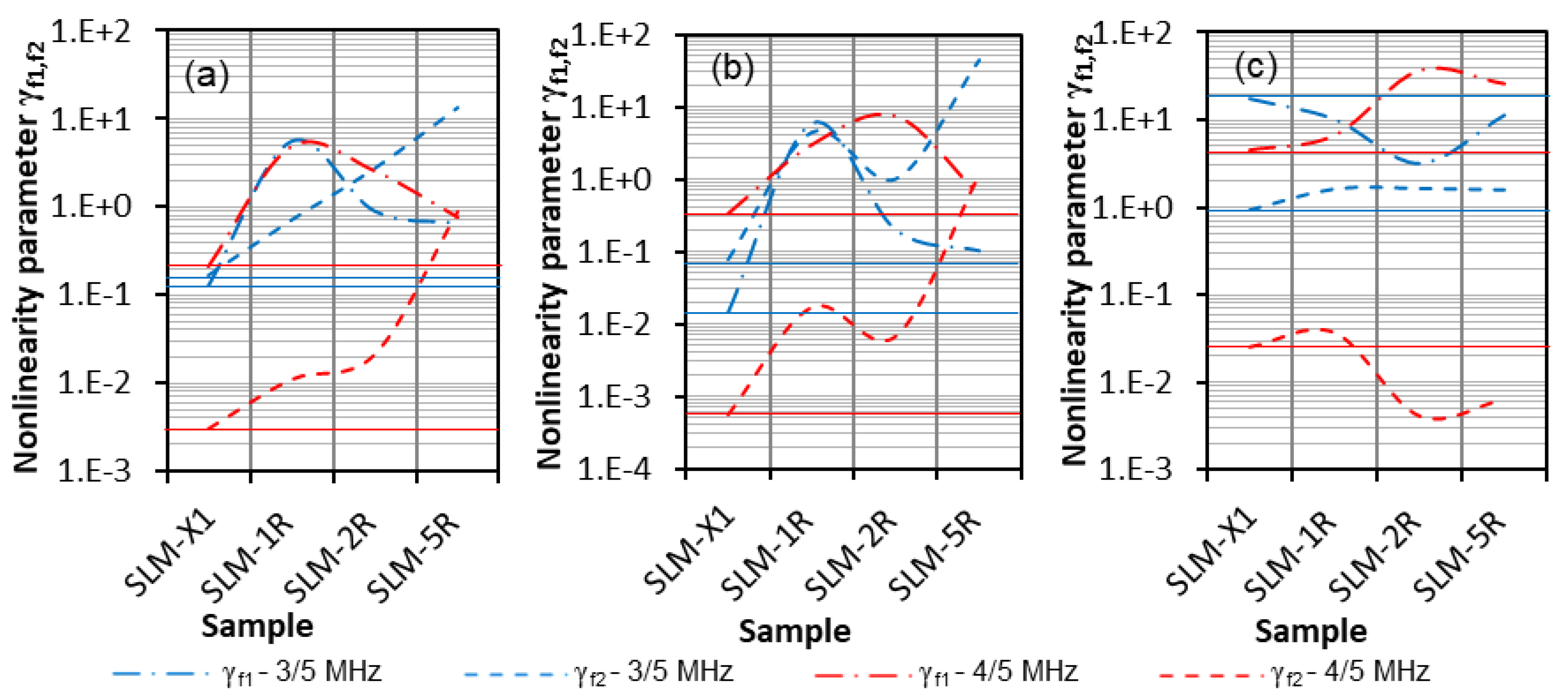
Figure 28.
Vane sample (III.7) with eroded defect.
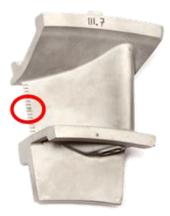
Figure 29.
Nonlinearity parameter, parallel sensor orientation, f1 = 4 MHz, f2 = 5 MHz: (a) Sensor orientation; (b) Experimental setup; (c) Comparison of nonlinearity parameter.
Figure 29.
Nonlinearity parameter, parallel sensor orientation, f1 = 4 MHz, f2 = 5 MHz: (a) Sensor orientation; (b) Experimental setup; (c) Comparison of nonlinearity parameter.
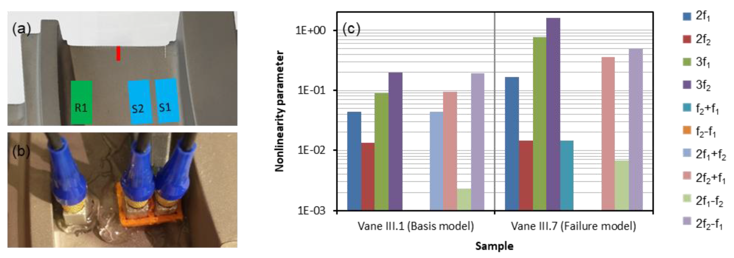
Figure 30.
Nonlinearity parameter, 90° sensor orientation, f1 = 4 MHz, f2 = 5 MHz: (a) Sensor orientation; (b) Experimental setup; (c) Comparison of nonlinearity parameter.
Figure 30.
Nonlinearity parameter, 90° sensor orientation, f1 = 4 MHz, f2 = 5 MHz: (a) Sensor orientation; (b) Experimental setup; (c) Comparison of nonlinearity parameter.

Figure 31.
Nonlinearity parameter, opposite sensor orientation, f1 = 4 MHz, f2 = 5 MHz: (a) Sensor orientation; (b) Experimental setup; (c) Comparison of nonlinearity parameter.
Figure 31.
Nonlinearity parameter, opposite sensor orientation, f1 = 4 MHz, f2 = 5 MHz: (a) Sensor orientation; (b) Experimental setup; (c) Comparison of nonlinearity parameter.
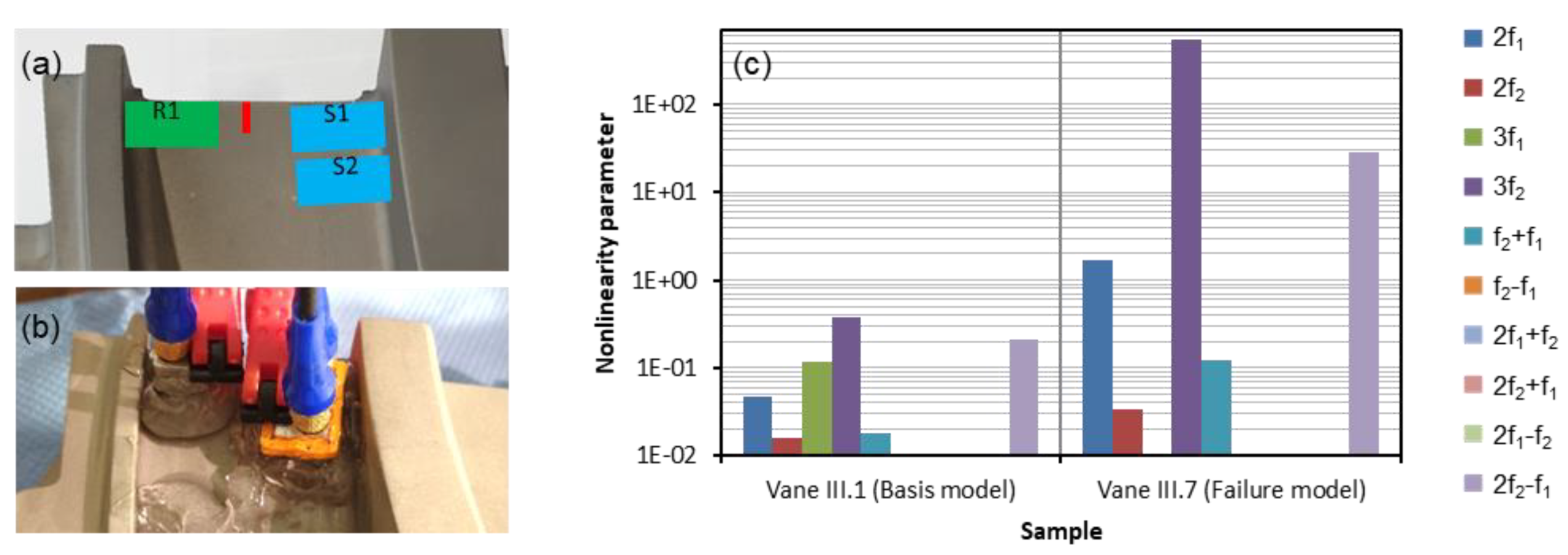
Figure 32.
Turbine blade (B286) with a crack on the trailing edge.
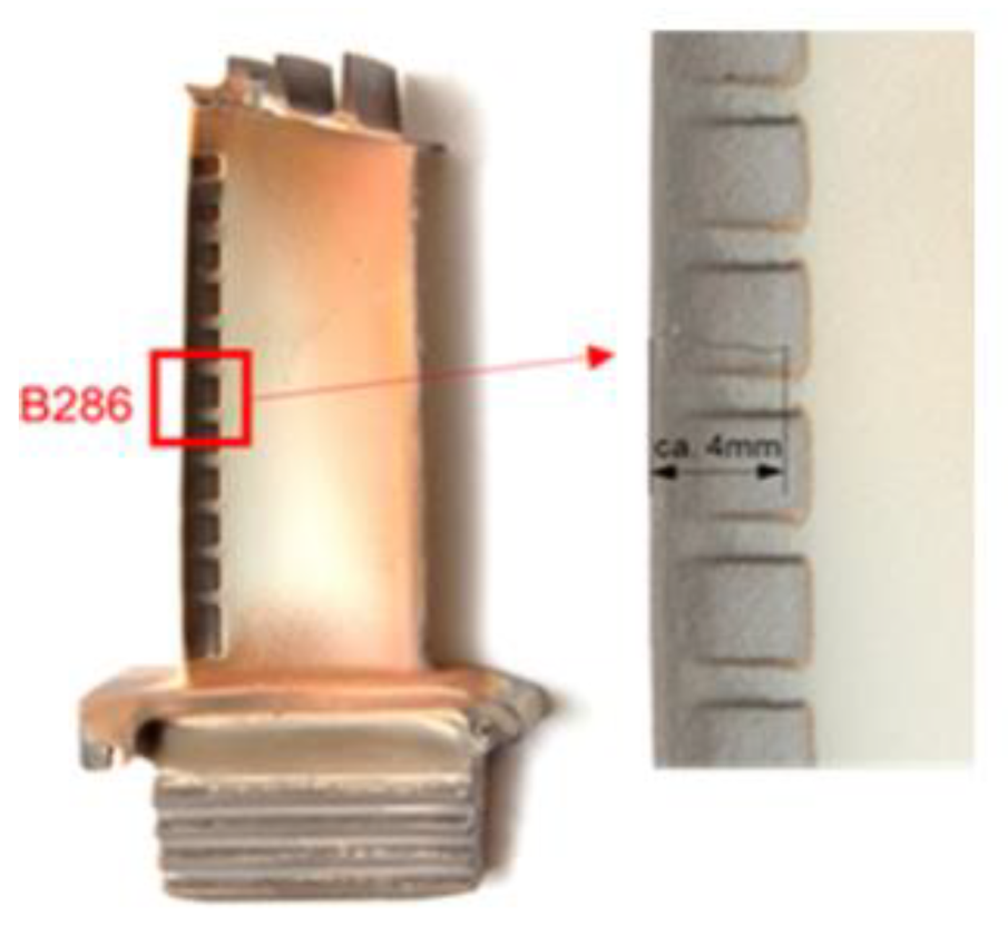
Figure 33.
Nonlinearity parameter: (a) f1 = 4 MHz, f2 = 5 MHz, α = 45°; (b) f1 = 4 MHz, f2 = 5 MHz, α = 60°; (c) f1 = 4 MHz, f2 = 5 MHz, α = 90°; (d) Sensor orientation; (e) Experimental setup.
Figure 33.
Nonlinearity parameter: (a) f1 = 4 MHz, f2 = 5 MHz, α = 45°; (b) f1 = 4 MHz, f2 = 5 MHz, α = 60°; (c) f1 = 4 MHz, f2 = 5 MHz, α = 90°; (d) Sensor orientation; (e) Experimental setup.

Table 1.
Summary modes.
| Mode | Frequency |
|---|---|
| n1 | f1 |
| n2 | f2 |
| n3 | 2f1 |
| n4 | 2f2 |
| n5 | 3f1 |
| n6 | 3f2 |
| n7 | f2 + f1 |
| n8 | f2 − f1 |
| n9 | 2f1 + f2 |
| n10 | 2f1 − f2 |
| n11 | 2f2 + f1 |
| n12 | 2f2 − f1 |
Table 2.
Material properties Inconel 718.
| Material | Inconel 718 |
|---|---|
| Density, ρ | 8.2 kg/dm3 |
| Speed of sound, c | 5820 m/s |
| Young’s modulus, E | 205,000 MPa |
| Poisson’s ratio, υ | 0.292 |
Table 3.
Welded plate specimens.
| Specimen | Crack Length | Crack Position |
|---|---|---|
| X1 | - | - |
| 1M | 1 mm | Centre |
| 1R | 1 mm | Lateral |
| 2M | 2 mm | Centre |
| 2R | 2 mm | Lateral |
| 5M | 5 mm | Centre |
| 5R | 5 mm | Lateral |
Table 4.
SLM manufactured metal specimens.
| Specimen | Crack Length | Crack Position |
|---|---|---|
| SLM-X1 | - | - |
| SLM-1R | 1 mm | Lateral |
| SLM-2R | 2 mm | Lateral |
| SLM-5R | 5 mm | Lateral |
© 2020 by the authors. Licensee MDPI, Basel, Switzerland. This article is an open access article distributed under the terms and conditions of the Creative Commons Attribution (CC BY) license (http://creativecommons.org/licenses/by/4.0/).
Share and Cite
MDPI and ACS Style
Mevissen, F.; Meo, M. A Nonlinear Ultrasonic Modulation Method for Crack Detection in Turbine Blades. Aerospace 2020, 7, 72. https://doi.org/10.3390/aerospace7060072
AMA Style
Mevissen F, Meo M. A Nonlinear Ultrasonic Modulation Method for Crack Detection in Turbine Blades. Aerospace. 2020; 7(6):72. https://doi.org/10.3390/aerospace7060072
Chicago/Turabian StyleMevissen, Frank, and Michele Meo. 2020. "A Nonlinear Ultrasonic Modulation Method for Crack Detection in Turbine Blades" Aerospace 7, no. 6: 72. https://doi.org/10.3390/aerospace7060072
Note that from the first issue of 2016, this journal uses article numbers instead of page numbers. See further details here.