Environment for Planning Unmanned Aerial Vehicles Operations


Department of Innovation Engineering, University of Salento, 73100 Lecce, Italy
*
Author to whom correspondence should be addressed.
†
These authors contributed equally to this work.
Aerospace 2019, 6(5), 51; https://doi.org/10.3390/aerospace6050051
Submission received: 28 February 2019
/
Revised: 29 April 2019
/
Accepted: 30 April 2019
/
Published: 4 May 2019
(This article belongs to the Special Issue Managing Data and Information of Aerospace Product Lifecycle)
Abstract
:Planning and executing missions in terms of trajectory generation are challenging problems in the operational phase of unmanned aerial vehicles (UAVs) lifecycle. The growing adoption of UAVs in several civil applications requires the definition of precise procedures and tools to safely manage UAV missions that may involve flight over populated areas. The paper aims at providing a contribution toward the definition of a reliable environment, called FLIP (flight planner) for route planning and risk evaluation in the framework of mini- and micro-UAV missions over populated areas. The environment represents a decision support system (DSS) for UAV operators and other decision makers, like airports authorities and aviation agencies. A new ICT tool integrating an innovative procedure for evaluating the risk related to the use of UAV over populated areas is proposed.
1. Introduction
The paper presents an IT environment for managing unmanned aerial vehicles (UAVs) operations in civil applications. The environment features functionalities, which encompass the entire operation cycle, from mission planning down to all relevant lifecycle data, and ensure the respect of appropriate safety levels.
Planning missions in terms of trajectory generation and executing them with adequate accuracy and safety levels are challenging problems in the operational phase of UAVs lifecycle [1] that require careful consideration. Studies were devoted to the life cycle of UAVs from the point of view of product development [2] and in particular structure design [3], design optimization [4], modeling and simulation [5]. To the best of the authors’ knowledge, the operational phase, including mission planning, has not been considered yet in the available literature. Filling this gap provides a relevant field of research for the community and the most relevant contribution of the present paper.
UAVs has been employed in various military tasks for a long time, such as surveillance and reconnaissance, penetration of enemy lines and weapon delivery [6]. A great deal of experience has thus been achieved in the last decades in operating this unconventional class of flying vehicle in restricted or inaccessible areas, such as military ranges or battlefields, with limited (if any) concern for public safety, in a scenario where mission effectiveness is more crucial than vehicle reliability.
At the same time, an ever-increasing range of potential civil applications for drones is being envisaged [6], where safety concerns represent a bottleneck to the actual development of a potentially huge market. Drones are already employed in those applications where the possibility of causing harm to third parties in case of failure is negligible, such as disaster monitoring and relief or precision farming. Other applications, such as parcel delivery or surveillance, require careful consideration of the risk related to the use of drones over populated areas. Moreover, strict procedures need to be enforced, in order to avoid interference with conventional air traffic, before drones are allowed to be flown in the civil airspace [7].
Risk assessment, hence, represents one of the most crucial issues in developing procedures for allowing safe UAV operations in civil application over populated areas, from both the regulatory [8], and the mission planning points of view. In this latter framework, several studies have been devoted in the last 20 years to evaluating the risk for the population due to ground impact of UAVs after failure [9,10,11,12,13,14,15,16]. The concept of a lethal area was introduced with the objective of sizing the portion of ground surface where a drone can cause fatal injuries to a person who stays inside the area at the time of drone crash [8]. Most of the techniques discussed in the literature combined the size of the lethal area with density population for evaluating risk.
Assuming fatal injuries for all people inside the lethal area [9,10,11] may result in an unnecessarily over-conservative risk estimate, which in turn may produce unrealistic requirements on vehicle reliability. For this reason, a penetration factor [12,13] or a sheltering factor [14] were introduced, which account for the possibility of reducing risk if a portion of the population is inside buildings or somehow sheltered by features of the surrounding environment. The possibility of being sheltered obviously depends on the drone size and velocity at impact and the factor may be strongly time dependent on both daily, weekly or seasonal time-scales. Lum et al. [15] combined all the above-mentioned concepts, including statistical analysis of potential impact points.
All these works emphasize what happens around the impact point, thus providing a risk analysis when a failure occurs at a given point along the mission flight path. In a recent paper [16] a global risk analysis for the entire mission was proposed, by adopting both a deterministic approach, where the position of the vehicle along the nominal trajectory at the time of failure is assumed known, and a statistical approach, where the effect of navigation errors is included in the analysis and a distribution of possible impact point is dealt with.
Mission trajectory is discretized by means of motion primitives, that is, segments or arcs that the vehicle can fly in a steady state condition. This allows to describe the whole trajectory by means of a limited number of parameters, namely four NP, if NP is the number of primitives used. For a given trajectory, the corridor swept on the ground by either the lethal area (for the deterministic approach) or the statistical impact footprint (for the statistical approach) is identified and a measure of risk is obtained, which depends on vehicle reliability and population density inside the corridor, which may vary along the trajectory. Given the limited number of variables necessary for describing the whole trajectory, this approach lends itself to be used within an optimization procedure, for the design of mission trajectories with an acceptable risk level [17].
The present paper aims at providing a further step toward the definition of a reliable environment, called FLIP (flight planner) for path planning and risk evaluation in the framework of mini- and micro-UAS missions over populated areas. The environment represents a modular decision support system (DSS) for UAV operators and other decision makers, like airports authorities and aviation agencies.
DSSs are information systems that support decision-making [18]. The main characteristics are as follows: DSSs incorporate both data and mathematical models. DSSs objective is to improve the effectiveness of the decisions, providing support for decision makers mainly in semi-structured and unstructured situations by bringing together human judgment and computerized information. DSSs must be designed to interact directly with the decision maker in such a way that the user has a flexible choice and a sequence of knowledge management activities [19]. The major components of a DSS architecture are the database (or knowledge base) storing the input and output data, the models and analytical tools, and the user interface [20,21]. Some scholars consider the users themselves as components of the architecture [18].
There is an extensive literature on DSSs, developed for almost every knowledge domain. An interesting category is one of the spatial DSSs, which help decision-makers to solve complex problems related to geographic or spatial data [19]. In current literature, few DSS for UAV operations exist. They have been developed for disaster monitoring [22,23,24,25,26], agricultural and forest applications [27,28], air traffic management [29], multi UAVs operations planning [30] and monitoring [31]. To the best of the authors’ knowledge, none of the existing systems supports decision makers to define flight routes using risk minimization as the path optimization main criteria.
In the next paragraph, the FLIP environment is described in terms of activities and input data needed for mission planning. The risk assessment methodology and details about routes calculation and optimization are provided in Section 3. In Section 4, functional architecture and graphical interface of the FLIP environment are described. The achieved results in an applicative scenario and possible implications for the framework of product lifecycle management are discussed in Section 5. Finally, conclusions section ends the paper.
2. UAV Flight Planning Scenario
The UAV flight planning process starts with the request, by an operator, of planning a new mission. Depending on the operational scenario, this request can be performed to the manager of a flight test center, to an airport authority or to an aviation agency. The process presented here is independent of the specific operational context (e.g., test mission, surveillance mission, payload test) and of the business context and therefore of the actor who initiates the flight planning request (e.g., UAV manufacturer, UAV operator). The input data required for planning a UAV mission, by means of the FLIP environment, can be grouped into three main categories (Table 1):
- Data of the vehicle(s) involved;
- Data of the operation(s) to be performed;
- Data of the environment where the operation(s) will be performed.
The first dataset contains all the data that are necessary to define vehicles performance limitations. Among these data, there are, for instance, the aerodynamic drag polar and the maximum lift coefficients, the maximum structural load factor, and the maximum engine power or thrust. These data, that are usually known from the aircraft manufacturer or estimated early in the design process, are used to verify the feasibility of a given trajectory. Overall UAV reliability is another fundamental data that has a direct impact on mission risk level.
The second dataset contains data representing operational constraints, such as mission start and end points (most often coinciding for small UAVs), intermediate waypoints through which the trajectory must necessarily pass (e.g., points where the UAV has to carry out a photographic survey) and mission schedule (different areas can be more or less densely populated depending on the time of the day, day of the week and even season).
The third dataset contains data about the orographic characteristics, buildings, and obstacles of the operational area and expected population density (possibly in a dynamic fashion). By sampling the planned trajectory with a sufficiently fine spatial resolution, it is possible to guarantee that the altitude of the vehicle never falls below a safety margin above ground level. At the same time, minimum distance from obstacles can be evaluated and maintained above a prescribed safety threshold. All these aspects are nowadays common practice in trajectory planning algorithms. Their implementation is not discussed here, being out of the scopes of the paper. Finally, population density represents another fundamental ingredient for risk analysis in UAVs mission planning, by means of the FLIP environment. The distribution of the population is assumed known (although not at a dynamic level). In the present application, this information is made available on a discrete square grid, where the population is assumed uniformly distributed inside each grid element.
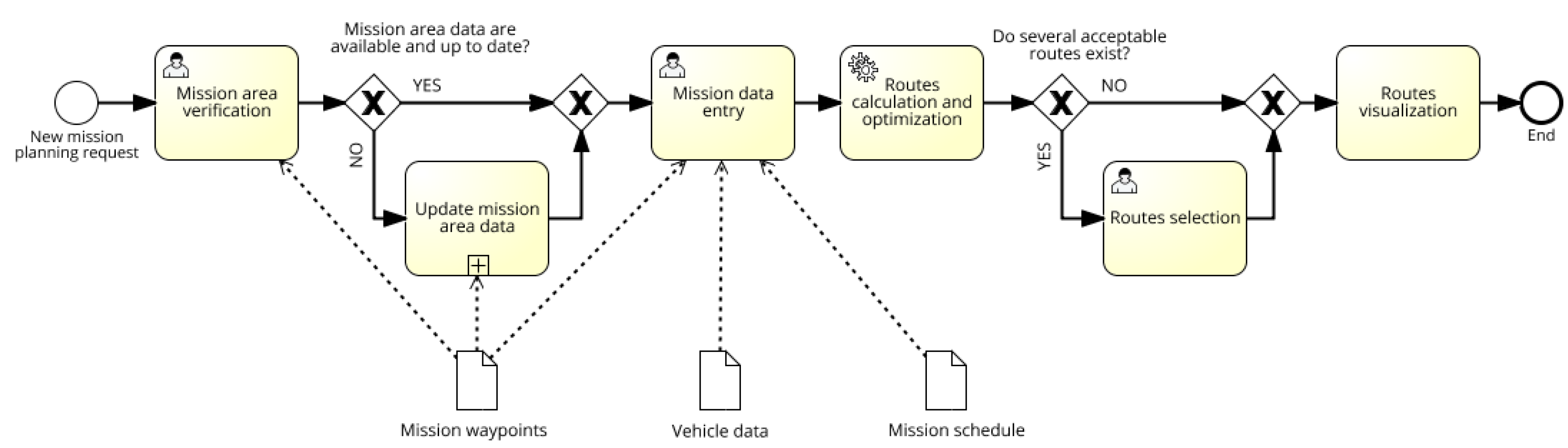
Figure 1 illustrates the FLIP activities workflow.
The first step consists in verifying, on the basis of the mission data provided (i.e., start point, end point, waypoints) if the flight area has been already analyzed and if the available data are up to date. If the data are unavailable or are not up to date, it is necessary to (re)analyze the area and (re)create the relevant maps, updating the presence of obstacles, new buildings, streets and the distribution of population density. Once done, the UAV operator is expected to provide the data on vehicle and operation schedule. Once all input data are available, the optimization algorithm boundary conditions can be set, and the simulation launched.
If only one route is found, with an associated risk below the acceptable risk threshold, it can be directly represented in the visualization module, otherwise, the operator can be offered a set of viable alternatives. When more routes are available, it is possible to display only one or two of them (e.g., the minimum risk trajectory, and/or the minimum flight time among acceptable routes, according to the selected optimization criteria) or let the operator free to choose among the available options, on the basis of his/her own operational considerations.
3. Routes Calculation and Optimization: The Risk Assessment Methodology
The tool developed for risk analysis within the FLIP environment implements the approach and methods presented in [16]. Its most relevant features are briefly recalled here in a rigorous, yet mostly qualitative, fashion. The reader is referred to the original paper, for more mathematical details and a complete description of the method.
3.1. Motion Primitives and Trajectory Discretization
In order to design the whole trajectory by means of a limited number of parameters, an approach originally proposed for robotic applications is developed [32], based on the notion of motion primitive. A motion primitive is the trajectory that a vehicle can follow in a steady state condition. It is possible to prove that flying vehicles at trim (that is, when forces and moments are balanced) follow either a straight (possibly climbing or descending) flight path or a steady turn [33]. When the turn is at a constant altitude, the resulting trajectory is a circular arc, whereas for climbing or descending turns the trajectory becomes a helix. This property holds for fixed-wing aircraft as well as for rotorcraft.
A total of three kinematic variables, all constant at steady state, namely airspeed V, climb rate dh/dt (or equivalently climb angle, γ), and turn rate Ω fully describe the steady state condition. If the mission trajectory is discretized by means of NP motion primitive elements (arcs or segments), each element is univocally defined by the three kinematic variables plus a fourth parameter, either a time interval Δt or arc-length Δs counted along the trajectory, which determines its size. A total of four NP + four parameters is thus sufficient for identifying the whole trajectory, where the four additional parameters are represented by three coordinates of the starting point and an initial value for the course angle.
3.2. Trajectory Feasibility
A trajectory is:
- (1)
- geometrically feasible if it does not interfere with obstacles and terrain;
- (2)
- dynamically feasible if every motion primitive can be flown by the vehicle without violating aerodynamic, structural or propulsion performance limits.
In order to assess feasibility with respect to geometric features of the environment, a map is required, with sufficient details on buildings and other obstacles. The trajectory is discretized, with sufficient spatial resolution, in order to evaluate the minimum distance from obstacles and from waypoints (if required by the particular mission) [17]. A trajectory is geometrically acceptable if
- (a)
- minimum altitude above the ground is greater than a prescribed clearance, which accounts for most of the obstacles (such as buildings, trees);
- (b)
- distance from high obstacles (communication towers, power lines, isolated trees) is greater than a prescribed safety threshold;
- (c)
- minimum distance from waypoints that need to be flown over during the mission is below a prescribed accuracy threshold.
Safety and accuracy threshold may depend on the particular vehicle and/or sensor used. As an example, the safety threshold from obstacles needs to account for vehicle size (wingspan or rotor diameter, plus a safety margin). Similarly, the accuracy threshold for navigating the vehicle over waypoints may depend on the width of the field of view of the sensor used for the mission. Apart from these aspects, geometric feasibility does not depend on the particular vehicle used.
Conversely, dynamic feasibility of all motion primitives clearly depends on performance capabilities of the vehicle, hence on its aerodynamic, structural and propulsion characteristics and configuration.
For fixed-wing propeller driven UAVs, a motion primitive is feasible if
- (a)
- power required for flying the trajectory arc, Pr, is smaller than the maximum available power, Pr ≤ ηP × Pmax, where ηP is propeller efficiency and Pmax is the maximum power delivered by the engine;
- (b)
- the wing lift coefficient CL is sufficiently far from stall, CL ≤ CLmax;
- (c)
- the normal load factor nz required in turning motion primitives is smaller than the maximum structural design maximum load factor, nz ≤ nz,max.
The load factor only depends on the three kinematic parameters which describe the trajectory arc, V, γ, and Ω, being
- nz = cosγ ≈ 1 in straight flight;
- nz = 1 + (Ω × V/g)2 in turning flight.
where g is gravity acceleration. Once nz is known, lift coefficient and required power are equal to [34]
- CL = nz × W/(½ρ × V3 × S)
- Pr = ½ρ × V3 × S × CD + W × V × sinγ
where W and S are vehicle weight, and wing planform area, respectively, and a parabolic drag polar is adopted for estimating the drag coefficient, CD = CD0 + KCL2, far from stall. All the inequality constraints at points (a), (b) and (c) can thus be easily evaluated from the three parameters of each trajectory arc (namely V, γ, and Ω) and vehicle characteristics (engine, aerodynamic and structural load limits, Pmax, CLmax, and nz,max, vehicle weight W, and wing area S, aerodynamic drag coefficients CD0 and K, propeller efficiency, ηP). A trajectory is dynamically feasible if all the inequality constraints are satisfied for all primitive arcs along the considered trajectory. The transition from one primitive to the following one is not considered in the analysis.
For rotary wing aircraft, dynamic feasibility is mainly related to available engine power, which is required to remain greater than the sum of power required by the rotor(s), fuselage parasite power and climb power [34]. As far as vehicle parameters are concerned, required power depends on vehicle weight, fuselage parasite area, f, rotor geometric (number of blades, radius, and solidity) and aerodynamic (blade airfoil drag coefficient and lift gradient) characteristics. The resulting calculations are less trivial than that required for the fixed wing case, recalled above, and include an iterative process for the determination of rotor induced velocity. The procedure is outlined in sufficient detail in [35].
3.3. Risk Evaluation
In order to evaluate the total risk, the distribution of the population within the area of operations needs to be known. This relevant piece of information can be obtained by means of a combined approach based on satellite pictures, information from local authorities and in-situ inspections. Real-time estimate can be obtained if one has access to information such as mobile phone traffic [36]. This information is provided to the FLIP environment, as discussed above, in Section 2.
The risk evaluation procedure proposed in [16] hinges on the notions of risk corridor and exposed time. The extension AL of the lethal area depends on vehicle size (e.g., wing span b), kinetic energy (T = ½ × (W/g) × Vi 2) and glide angle (γi) at impact. Its position with respect to that of the vehicle at the time of catastrophic failure tcf depends on vehicle velocity V, course angle χ and altitude h at time tcf. The impact point is assumed to lie at the end of a parabolic fall trajectory. When population density ρP is uniform in the area of operations, the risk R is given by
where pF is the probability of a failure during vehicle operations and pI is the probability that vehicle impact inside the lethal area results into casualties and/or serious injuries.
R = pF × pI × AL × ρP
If one follows the nominal mission trajectory, the lethal area sweeps a corridor on the ground, which is referred to as the risk corridor. It is possible to prove that Equation (1) can be rearranged in such a way that the risk of hitting somebody is proportional to the time spent by a point on the surface inside the risk corridor (referred to as exposed time te) multiplied by the population density in that point and the total area spanned by the lethal area, that is, the area inside the risk corridor. Exposed time is evaluated for various shapes of the feasible motion primitives, but it mainly depends on vehicle airspeed, being roughly inversely proportional to V. Exposed time is constant along a rectilinear motion primitive. Although some variations of exposed time are present across the corridor width, for curved trajectory elements, it is possible to assume an approximately constant value of te also in the transverse direction, with minor errors, which barely affect the results when evaluating the total risk.
In order to obtain a numerically efficient risk evaluation algorithm, valid also for missions taking place over a wide zone where population density is not uniform, the area of operations is discretized by means of a regular grid. Inside each grid, element density is assumed constant. Grid elements which do not cross the risk corridor do not contribute to the total risk. If the risk corridor intersects one element, the contribution of the element to the total risk is proportional to the product of population density within the grid element times the exposed time times the size of the intersection of the grid element with the risk corridor. Assuming for the sake of simplicity that all impacts inside AL are lethal (that is, pI = 1), the total risk along the whole trajectory can be estimated as
where M is the number of grid elements crossed by the risk corridor, Sk and ρk are the surface of the risk corridor and population density inside the k-th grid element, respectively, te,k is the exposed time for points inside Sk, and tM is the total mission time.
Probability of vehicle failure, pF, multiplies the whole expression of risk. Vehicle reliability thus plays a decisive role: risk being proportional to the probability of a catastrophic failure that results in a total loss of control of the vehicle. A conservative risk estimate is derived assuming that failure occurs during the mission. If the total risk of providing damage to third parties is below an acceptable threshold, the actual risk is much lower. At the same time, if the risk is above the acceptable limit, whichever the trajectory, the factor required to bring risk below the threshold is inversely proportional to the number of missions that need to be flown without failure. This provides a requirement for vehicle reliability in terms of time-between-failures.
If navigation errors are included in the analysis, that is, failure occurs at a point which is not on the nominal trajectory, a statistical approach needs to be envisaged, which includes the effect of navigation errors on the impact point on the ground. The effect of navigation errors on the risk analysis is taken into consideration by determining a statistical impact footprint (SIF), that is, a 2-D distribution of impact points on the ground, starting from a nominal failure point (in terms of initial altitude and airspeed), and adding Gaussian distributions for vertical and lateral deviations from the prescribed flight path and velocity components with respect to the nominal value.
Monte Carlo simulation is used for determining the distribution of impact points. The statistical distribution is discretized by means of three ellipses, with semi-major axes proportional to the standard deviation σx and σy of the distance of impact points with respect to the nominal one in the along- and cross-track directions, respectively. The σ, 2-σ, and 3-σ ellipses respectively encompass 39.4%, 86.5% and 99% of total impact points. Three risk corridors are determined in a way similar to that derived for the lethal area, where an additional factor weights the total risk inside each corridor, which becomes proportional to the fraction of impact points inside the considered ellipse, but outside the inner one(s).
The two risk analysis approaches provide the same figure for total risk if population density is uniform. Some differences emerge if large density gradients are present, in which case the (usually narrower) lethal area risk corridor may underestimate risk. The SIF approach can be extended also to different fall scenarios, such as gliding descent of a fixed wing vehicle after an engine failure, in which case the width of the risk corridor may become large, thus making the identification of a safe trajectory difficult, over densely populated areas. A convenient evaluation of the sheltering factor may at least partially mitigate this problem, but this is out of the scopes of the present paper.
4. The FLIP Environment
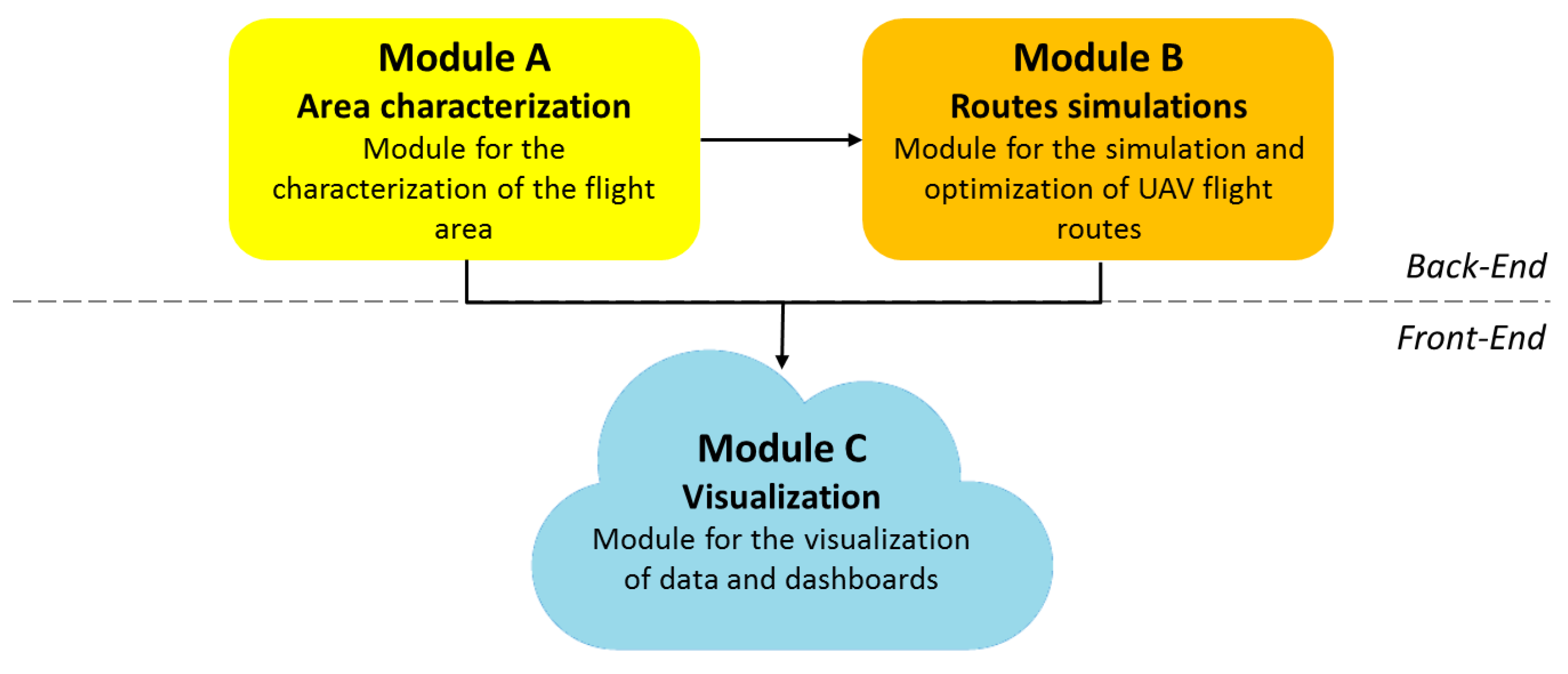
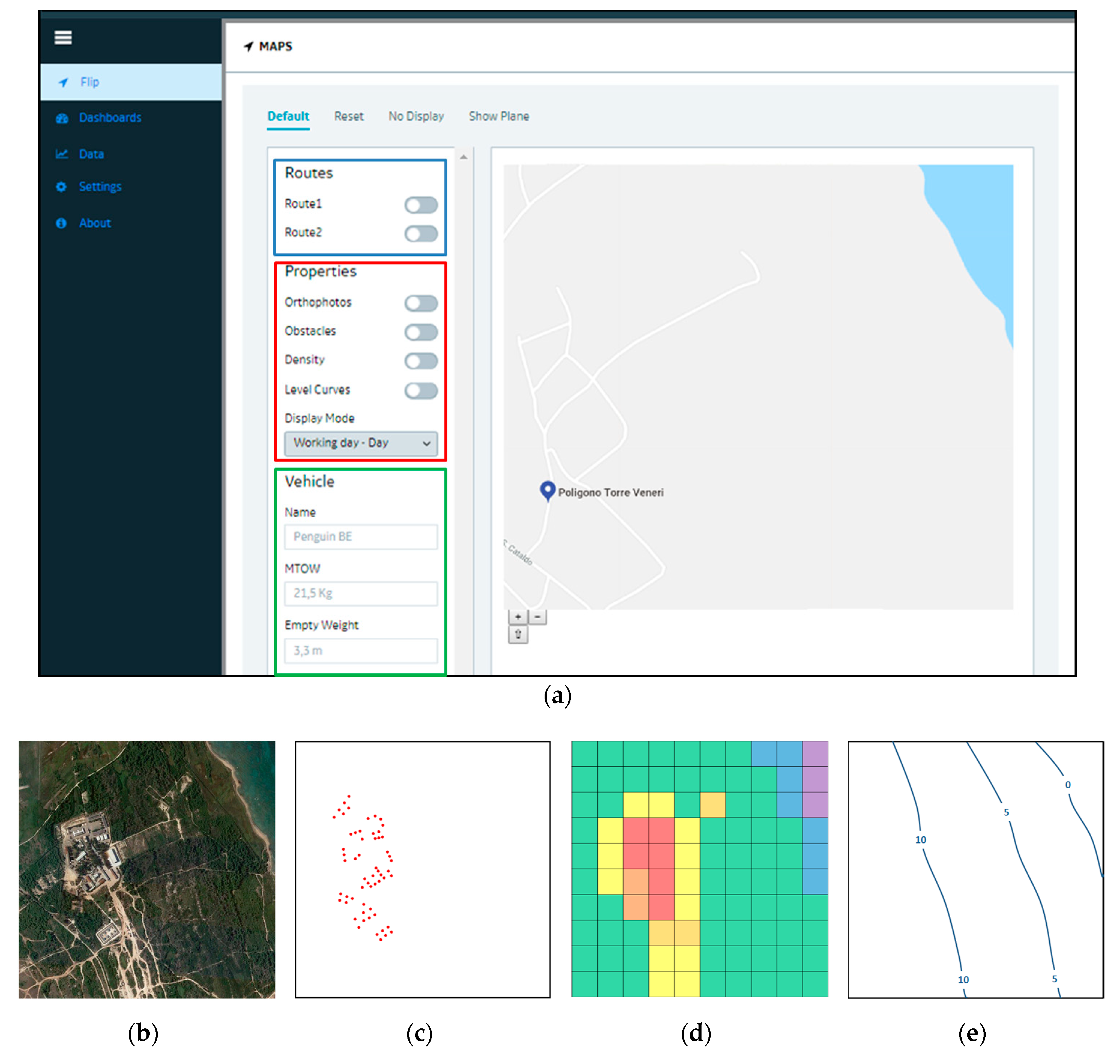
From a functional point of view, the FLIP modules follow a user-centric approach, providing an environment accessible to users (e.g., UAV operators) through front-end and back-end components of the system. Referring to Figure 2, Module A allows the management and analysis of input data characterizing the flight area in terms of orographic characteristics, buildings, obstacles, and population density. Module B implemented the algorithms, presented in Section 3, for the analysis (and possibly optimization) of flight routes minimizing the risk of the mission. Finally, Module C represents the single front-end component for the visualization and analysis, through a web interface, of the output data of the FLIP process, i.e., the results of the numerical elaboration for the calculation of the risk, the trajectories that minimizes it, as well as all the main input data used for the simulation. The data are extracted and exchanged through the different modules by means of APIs and web-services. An explanatory screenshot of the developed web application is provided in Figure 3.
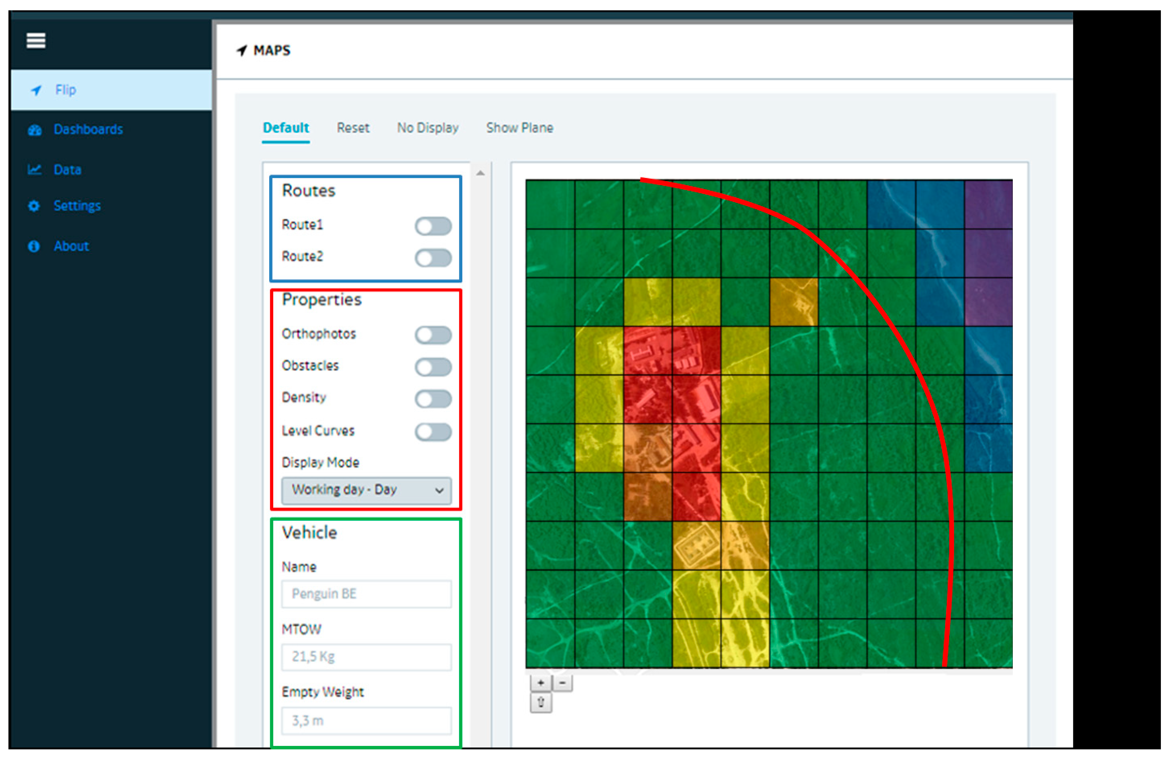
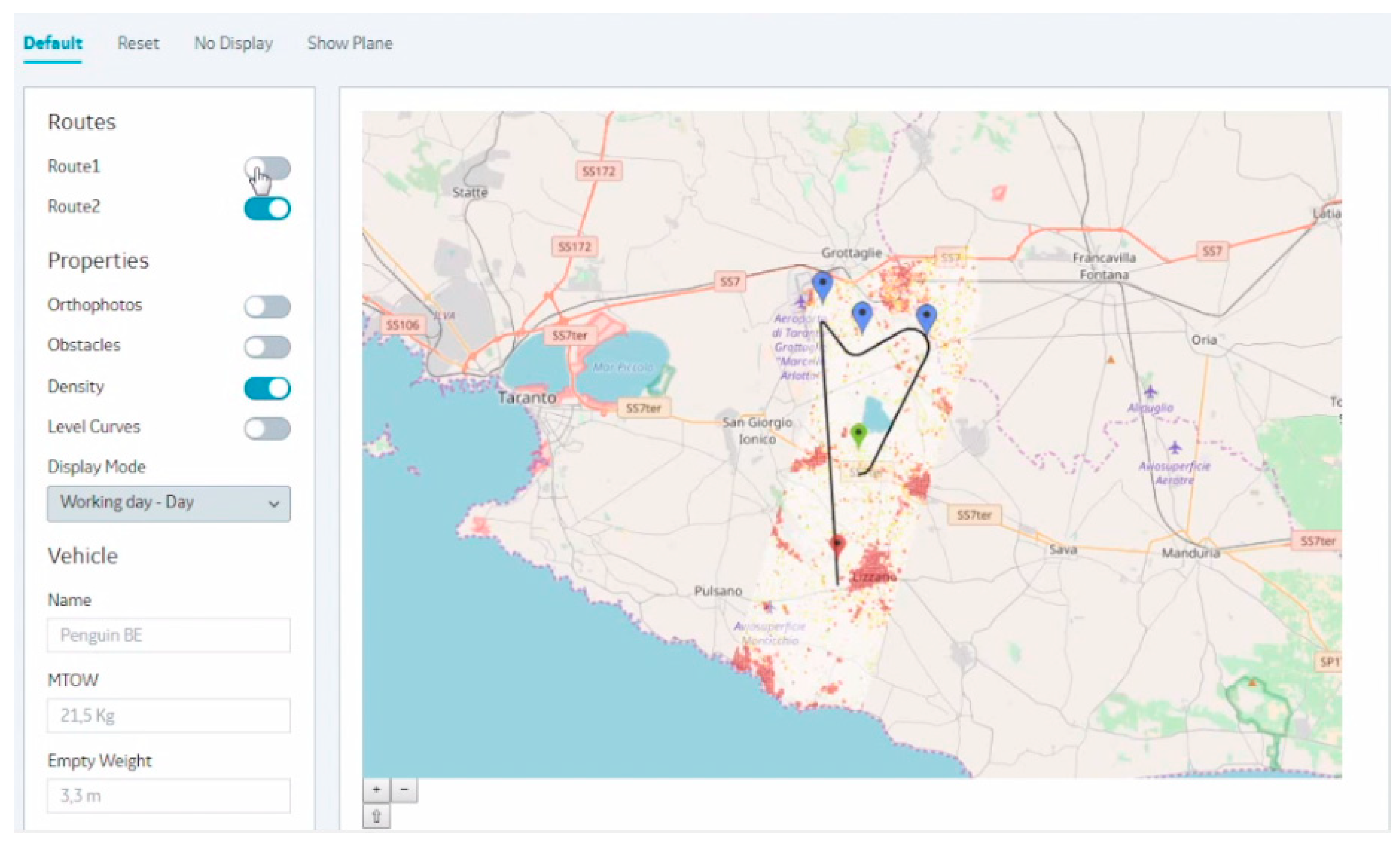
Five different views are available: (1) map view, (2) orthophoto view, (3) obstacle map, (4) population density grid and (5) level curves view. Each view can be turned on/off by means of switches in the red area of the graphical user interface (GUI). The switches in the blue area of the GUI are used to turn on/off the display of one or more routes calculated using the risk analysis algorithm. Different visualization view can be combined, in different layers, as desired, as shown in Figure 4, where Route 1, orthophoto view and population density map are simultaneously turned on. The green area of graphical interface reports some data about the vehicle under consideration that has been used for the trajectory definition and related risk calculation.
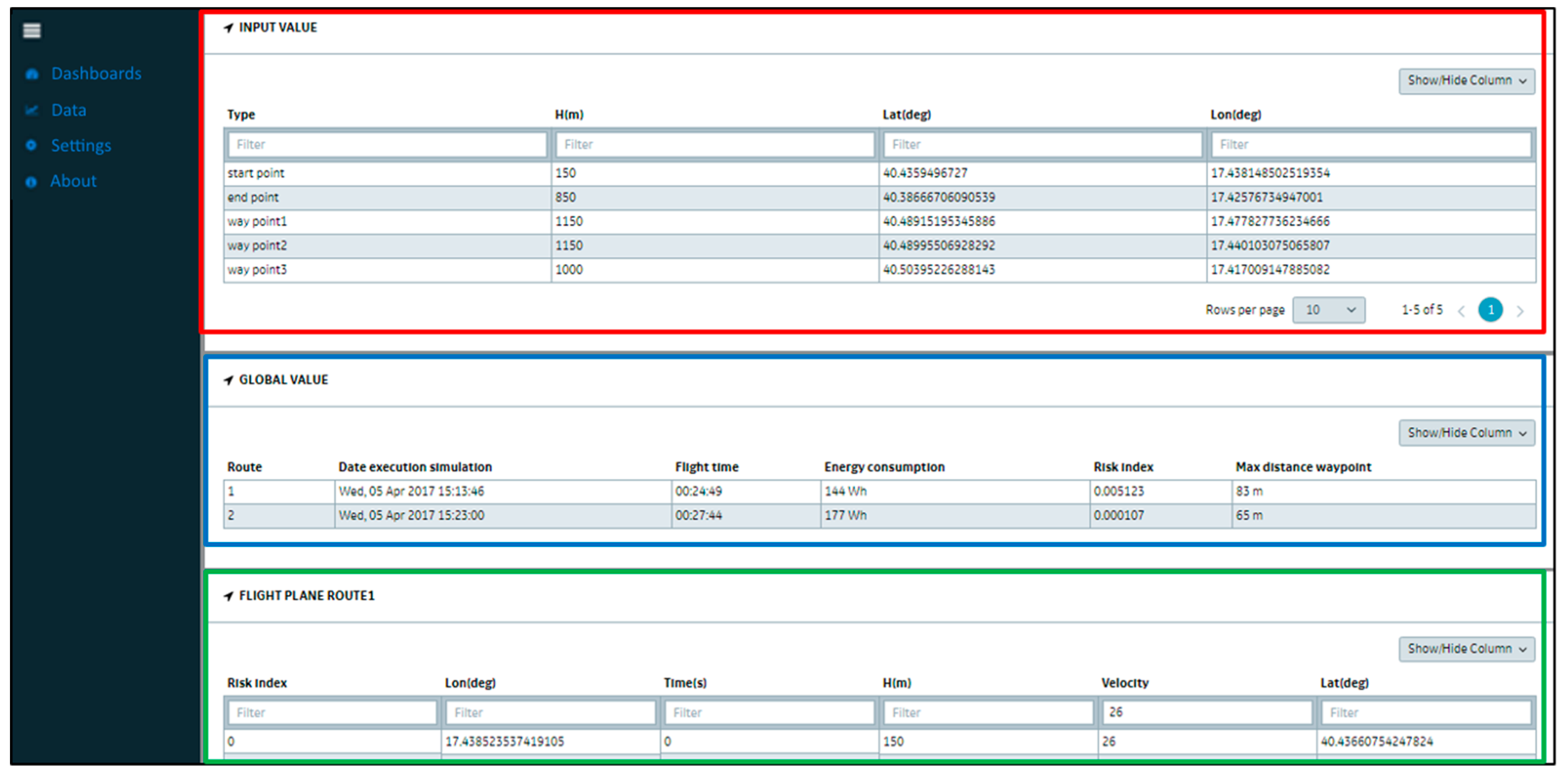
Another section of the FLIP application is dedicated to the visualization of detail data in numerical format (Figure 5). Height, longitude and latitude of the input points used for the design of the trajectory (i.e., start point, end point, and intermediate waypoints) and global performance indexes for the proposed routes (i.e., flight time, energy consumption, risk index, and maximum distance from waypoints) are reported respectively in the red and the blue sections.
Finally, in the green area the single points of the selected trajectory, sampled at 1 Hz, are reported. The points visualized on the screen can be filtered according to risk index, longitude, latitude, time, velocity, height. These data can be used in the visualization tool to analyze in depth the properties of the proposed route(s), also representing the second output of the FLIP process. These points, appropriately resampled (e.g., with a frequency different from that used in the visualization tool, or with completely different sampling criteria), can be used for programming the autonomous flight of the UAV.
5. Test and Discussion
The FLIP environment was demonstrated in an applicative scenario for a small-scale UAV in the framework of a research program. The characteristics of the vehicle are summarized in Table 2. A mission with X waypoints in the area surrounding Grottaglie airport (near Taranto, in Southern Italy) was envisaged as a representative operational scenario for testing the tools in a realistic situation. Population density data were supplied by one of the project partners, whereas a general purpose multi-objective search algorithm, developed by another partner, was used for enforcing mission constraints and minimize risk [17].
For the given start point (green placeholder), end point (red placeholder) and mission waypoints (blue placeholder), the optimal route minimizing risk has been calculated. This is shown in Figure 6 in the web interface of the FLIP environment. The resulting optimal flight path is represented on the population density map overlaying an open-source map (OpenStreetMap ©), but the FLIP GUI allows the operator to switch from a visualization layer (i.e., density data) to others (i.e., orthophoto, obstacle map, level curves).
Managing mission planning input data and resulting trajectory in the FLIP environment covers the management of lifecycle data that are not managed in other systems currently adopted in the aerospace and defence industry. In this sense, the FLIP environment becomes part of the PLM strategy of a UAV producer, tester and user.
Aerospace and defence industry is the traditional sector in which PLM methodologies and technologies have been developed and adopted. The increasing product complexity and the growth of the design time required methods, process, and tools that let the engineers shorten development timeframes [37]. Product lifecycle management (PLM) is the business activity of managing, in the most effective way, company’s products all the way across their lifecycle. It is a strategic business approach and enables organizations to collaborate within and across the extended enterprise, integrating people, processes, and technologies [38,39]. Providing a unique and timed product data source PLM assures information consistency, traceability, and long-term archiving [40]. Product Lifecycle Management Systems (PLMS) are tools that implement the PLM concept. PLMS have long been focused on the area of planning, design and engineering functions [41]. Nowadays they try to cover more and more of the whole product lifecycle “from cradle to grave” [42] starting from operations and test activities. These are crucial phases in UAV lifecycle and include both testing activities and real mission execution.
Testing activities consist of flight to test the vehicle (or a specific payload), its performance and capabilities and to test its effectiveness in performing specific missions (e.g., surveillance, product deliveries, aerial photograph). Typical test activities include: vehicle performance assessment, in-flight vehicle checkout, testing payload or instruments, collecting and analyzing mission data, operators, and maintenance training.
The management of these data allows UAV designers, producers and users to exploit them even for scope other than mission planning. For instance, the trajectory data can be used, during the UAV testing phase, to store the testing conditions (e.g., climb rate) and to later compare them with data acquired by sensors used during the flight.
6. Conclusions
The introduction of UAVs in the civil airspace requires the definition of precise procedures and tools to safely manage UAV missions that may involve flight over populated areas. The paper presented an IT environment, called Flight Planner (FLIP), for planning unmanned aerial vehicles (UAVs) operations and managing relevant lifecycle data in respect of appropriate safety levels. The environment represents a decision support system (DSS) for UAV operators and other decision makers, like airports authorities and aviation agencies.
Data about the vehicle involved, the mission to be performed (i.e., operational constraints and mission schedule) and the environment where the mission will be performed represents the set of required inputs for calculating the routes. In particular, the distribution of the population within the area of operations is used for risk assessment. The proposed risk assessment methodology uses motion primitives for trajectory discretization, evaluates trajectory feasibility and assesses the associated risk.
The output data of the FLIP process are twofold: on the one hand, there are dashboards and data (visualized in the graphical interface) that supports UAV operator in-flight mission planning and, on the other hand, there are the optimal trajectory data that can be integrated into the autopilot of the UAV for its autonomous flight. In this sense, with further development, the FLIP environment could be used to monitor, in real time, the flight of a UAV, and to compare the trajectory actually performed with the planned one. The FLIP technological architecture, being modular and service-oriented, is already suitable for such an improvement.
Author Contributions
Supervision, A.C.; validation, G.A.; writing—original draft, C.P., M.M. and G.A.; writing—review and editing, C.P., M.M., G.A. and A.C.
Funding
This research was funded by the European Union and the Regione Puglia Local Government through call FSC Cluster 2014, project Test and Knowledge-based Environment for Operations, Flight and Facility (TAKE OFF).
Acknowledgments
The authors would like to thank all the TAKE-OFF project partners, for their valuable contributions to the study. In particular, the authors acknowledge EnginSoft Spa for the development of the multi-objective search algorithm, and Planetek Italia Srl for providing population density data.
Conflicts of Interest
The authors declare no conflict of interest.
References
- Valavanis, K.P.; Vachtsevanos, G.J. Uav mission and path planning: Introduction. In Handbook of Unmanned Aerial Vehicles; Springer: Berlin, Germany, 2015; pp. 1443–1446. [Google Scholar]
- Idries, A.; Mohamed, N.; Jawhar, I.; Mohamed, F.; Al-Jaroodi, J. Challenges of developing UAV applications: A project management view. In Proceedings of the the 2015 International Conference on Industrial Engineering and Operations Management (IEOM), Dubai, UAE, 3–5 March 2015; pp. 1–10. [Google Scholar]
- Vasić, Z.; Maksimović, S.; Georgijević, D. Applied integrated design in composite UAV development. Appl. Compos. Mater. 2018, 25, 221–236. [Google Scholar] [CrossRef]
- Gusev, M.P.; Nikolaev, S.M.; Uzhinsky, I.K.; Padalitsa, D.I.; Mozhenkov, E.R. Application of Optimization in the Early Stages of Product Development, Using a Small UAV Case Study. In IFIP International Conference on Product Lifecycle Management; Springer: Berlin, Germany, 2018; pp. 294–303. [Google Scholar]
- Bernabei, G.; Sassanelli, C.; Corallo, A.; Lazoi, M. A PLM-Based Approach for Un-manned Air System Design: A Proposal. In International Workshop on Modelling and Simulation for Autonomous Systems; Springer: Berlin, Germany, 2014; pp. 1–11. [Google Scholar]
- Holland Michel, A.; Gettinger, D. Drone Year in Review: 2017; Center for the Study of the Drone at Bard College: Washington, DC, USA, 2018. [Google Scholar]
- Guglieri, G.; Quagliotti, F.; Ristorto, G. Operational issues and assessment of risk for light UAVs. J. Unmanned Vehicle Syst. 2014, 2, 119–129. [Google Scholar] [CrossRef]
- Federal Aviation Authority. Flight safety Analysis Handbook; version 1.0; United States Department of Transportation: Washington, DC, USA, 2011.
- McGeer, T.; Newcome, L.R.; Vagners, J. Quantitative risk management as a regulatory approach to civil UAVs. In Proceedings of the International Workshop on UAV Certification, Paris, France, 4 June 1999; pp. 1–11. [Google Scholar]
- Clothier, R.; Walker, R.; Fulton, N.; Campbell, D. A casualty risk analysis for unmanned aerial system (UAS) operations over inhabited areas. In Proceedings of the Second Australasian Unmanned Air Vehicle Conference, Melbourne, Australia, 19–22 March 2007; pp. 1–15. [Google Scholar]
- Clothier, R.A.; Walker, R.A. Determination and evaluation of UAV safety objectives. In Proceedings of the 21st International Unmanned Air Vehicle Systems Conference, Bristol, UK, 3–5 April 2006; pp. 18.1–18.16. [Google Scholar]
- Weibel, R.; Hansman, R.J. Safety considerations for operation of different classes of UAVs in the NAS. In Proceedings of the AIAA 3rd ‘‘Unmanned Unlimited’’ Technical Conference, Workshop and Exhibit, Chicago, IL, USA, 20–23 September 2004; pp. 1–11. [Google Scholar]
- Weibel, R.; Hansman, R.J. An integrated approach to evaluating risk mitigation measures for UAV operational concepts in the NAS. In Proceedings of the 4th Infotech@Aerospace Conference, Arlington, VA, USA, 26–29 September 2005; pp. 509–519. [Google Scholar]
- Dalamagkidis, K.; Valavanis, K.P.; Piegl, L.A. Evaluating the risk of unmanned aircraft ground impacts. In Proceedings of the 2008 Mediterranean Conference on Control and Automation MED’08, Ajaccio (Corsica), France, 25–27 June 2008; pp. 709–716. [Google Scholar]
- Lum, C.; Gauksheim, K.; Deseure, C.; Vagners, J.; McGeer, T. Assessing and estimating risk of operating unmanned aerial systems in populated areas. In Proceedings of the 11th AIAA Aviation Technology, Integration, and Operations (ATIO) Conference, Virginia Beach, VA, USA, 20–22 September 2011; pp. 1–13. [Google Scholar]
- Avanzini, G.; Martinez, D.S. Risk assessment in mission planning of uninhabited aerial vehicles. Proc. Inst. Mech. Eng. G 2019. [Google Scholar] [CrossRef]
- Martinez, D.S.; Avanzini, G.; Primavera, V.; Micchetti, F.; Pagone, S.; Di Martino, A.; Marra, M.; Pascarelli, C. Risk Mitigation for Unmanned Air Vehicles Mission Planning. In Proceedings of the CAE Conference, Vicenza, Italy, 6–7 November 2017. [Google Scholar]
- Sprague, R.H., Jr. A framework for the development of decision support systems. MIS Q. 1980, 4, 1–26. [Google Scholar] [CrossRef]
- Nižetić, I.; Fertalj, K.; Milašinović, B. An overview of decision support system concepts. In 18th International Conference on Information and Intelligent Systems; Faculty of Organization and Informatics: Varazdin, Croatia, 2007; pp. 251–256. [Google Scholar]
- Power, D.J. Decision Support Systems: Concepts and Resources for Managers; Greenwood Publishing Group: Westport, CT, USA, 2002. [Google Scholar]
- Asemi, A.; Safari, A.; Zavareh, A.A. The role of management information system (MIS) and Decision support system (DSS) for manager’s decision making process. Int. J. Bus. Manage. 2011, 6, 164–173. [Google Scholar] [CrossRef]
- Sherstjuk, V.; Zharikova, M.; Sokol, I. Forest Fire Monitoring System Based on UAV Team, Remote Sensing, and Image Processing. In Proceedings of the 2018 IEEE Second International Conference on Data Stream Mining & Processing (DSMP), Lviv, Ukraine, 21–25 August 2018; pp. 590–594. [Google Scholar]
- Fikar, C.; Gronalt, M.; Hirsch, P. A decision support system for coordinated disaster relief distribution. Expert Syst. Appl. 2016, 57, 104–116. [Google Scholar] [CrossRef]
- Cho, K.; Baltsavias, E.; Remondino, F.; Soergel, U.; Wakabayashi, H. Resilience against disasters using remote sensing and geoinformation technologies for rapid mapping and information dissemination (RAPIDMAP). In Proceedings of the 34th Asian Conference on Remote Sensing, Bali, Indonesia, 20–24 October 2013; pp. 3826–3833. [Google Scholar]
- Cho, K.; Wakabayashi, H.; Yang, C.H.; Soergel, U.; Lanaras, C.; Baltsavias, E.; Rupnik, E.; Nex, F.; Remondino, F. Rapidmap project for disaster monitoring. In Proceedings of the 35th Asian Conference on Remote Sensing (ACRS), Nay Pyi Taw, Myanmar, 27–31 October 2014. [Google Scholar]
- Baltsavias, E.; Cho, K.; Remondino, F.; Sörgel, U.; Wakabayashi, H. Rapidmap-Rapid mapping and information dissemination for disasters using remote sensing and geoinformation. Int. Arch. Photogramm. Remote Sens. Spat. Inform. Sci. 2013, 40, 31–35. [Google Scholar] [CrossRef]
- Katsigiannis, P.; Galanis, G.; Dimitrakos, A.; Tsakiridis, N.; Kalopesas, C.; Alexandridis, T.; Zalidis, G. Fusion of spatio-temporal UAV and proximal sensing data for an agricultural decision support system. In Fourth International Conference on Remote Sensing and Geoinformation of the Environment (RSCy2016); International Society for Optics and Photonics: Bellingham, WA, USA, 2016; Volume 9688, p. 96881R. [Google Scholar]
- Sterenczak, K.; Mroczek, P.; Jastrzebowski, S.; Krok, G.; Lisanczuk, M.; Klisz, M.; Kantorowicz, W. UAV and GIS Based Tool for Collection and Propagation of Seeds Material-First Results. ISPRS Int. Arch. Photogram. Remote Sens. Spat. Inform. Sci. 2016, 41, 663–667. [Google Scholar] [CrossRef]
- Insaurralde, C.C.; Blasch, E. Ontological knowledge representation for avionics decision-making support. In Proceedings of the 2016 IEEE/AIAA 35th Digital Avionics Systems Conference (DASC), Sacramento, CA, USA, 25–30 September 2016; pp. 1–8. [Google Scholar]
- Ramirez-Atencia, C.; Camacho, D. Extending QGroundControl for Automated Mission Planning of UAVs. Sensors 2018, 18, 2339. [Google Scholar] [CrossRef] [PubMed]
- Porat, T.; Oron-Gilad, T.; Rottem-Hovev, M.; Silbiger, J. Supervising and controlling unmanned systems: A multi-phase study with subject matter experts. Front. Psychol. 2016, 7, 568. [Google Scholar] [CrossRef] [PubMed]
- Frazzoli, E.; Dahleh, M.A.; Eric, F. Maneuver-based motion planning for nonlinear systems with symmetries. IEEE Trans. Robot. 2005, 21, 1077–1091. [Google Scholar] [CrossRef]
- Etkin, B. Dynamics of Atmospheric Flight; Wiley: New York, NY, USA, 1972. [Google Scholar]
- McCormick, B.W. Aerodynamics, Aeronautics, and Flight Mechanics; Wiley: New York, NY, USA, 1995. [Google Scholar]
- Avanzini, G.; Carlà, A.; Donateo, T. Parametric analysis of a hybrid power system for rotorcraft emergency landing sequence. Proc. Inst. Mech. Eng. G 2017, 231, 2282–2294. [Google Scholar] [CrossRef]
- Khodabandelou, G.; Gauthier, V.; El-Yacoubi, M.; Fiore, M. Population estimation from mobile network traffic metadata. In Proceedings of the IEEE 17th International Symposium on a World of Wireless, Mobile and Multimedia Networks (WoWMoM), Coimbra, Portugal, 21–24 June 2016. [Google Scholar]
- Mas, F.; Arista, R.; Oliva, M.; Hiebert, B.; Gilkerson, I.; Rios, J. A review of PLM impact on US and EU aerospace industry. Proc. Eng. 2015, 132, 1053–1060. [Google Scholar] [CrossRef]
- Product Lifecycle Management, Empowering the Future of Business. Available online: https://www.cimdata.com/en/resources/complimentary-reports-research/white-papers (accessed on 15 January 2019).
- Grieves, M. Product Lifecycle Management: Driving the Next Generation of Lean Thinking by Michael Grieves; McGraw-Hill: New York, NY, USA, 2006. [Google Scholar]
- Corallo, A.; Latino, M.E.; Lazoi, M.; Lettera, S.; Marra, M.; Verardi, S. Defining product lifecycle management: A journey across features, definitions, and concepts. ISRN Ind. Eng. 2013, 2013, 170812. [Google Scholar] [CrossRef]
- Haas, K.; Schuck, H.; Mücke, T.; Ovtcharova, J. A holistic product lifecycle management approach to support design by machine data. Proc. CIRP 2016, 50, 420–423. [Google Scholar] [CrossRef]
- Armstrong, S. Engineering and Product Development Management: The Holistic Approach; Cambridge University Press: Cambridge, UK, 2001. [Google Scholar]
Figure 1.
Flight planner (FLIP) process.

Figure 2.
FLIP functional architecture.

Figure 3.
FLIP dashboards: (a) Map view, (b) orthophoto view, (c) obstacles view, (d) population density view, (e) Isolevel curves view.
Figure 3.
FLIP dashboards: (a) Map view, (b) orthophoto view, (c) obstacles view, (d) population density view, (e) Isolevel curves view.

Figure 4.
Combination of different visualization layers in the FLIP dashboards.

Figure 5.
FLIP data visualization.

Figure 6.
Sample mission results.


Table 1.
Flight planner (FLIP) input data.
| Data of the Vehicles | Data of the Operation | Data of the Environment |
|---|---|---|
| Reliability | Start point | Orthophoto |
| Aerodynamic characteristics | End point | Orography |
| Structural performance limits | Waypoints | Obstacles |
| Propulsion performance limits | Schedule | Population density |
Table 2.
Aircraft data for sample mission.
| Parameter | Symbol | Value | Units |
|---|---|---|---|
| Takeoff weight (max.) | W | 21.5 | kg |
| Wing span | b | 3.3 | m |
| Wing area | S | 0.79 | m2 |
| Max. propulsion power | Ps,max | 2700 | W |
| Max. lift coefficient (clean) | CLmax | 1.3 | |
| Max. lift coefficient (with flap) | CLmax | 1.7 | |
| Drag polar coefficients (estimated from performance data) | CD0 | 0.05 | |
| K | 0.03 |
© 2019 by the authors. Licensee MDPI, Basel, Switzerland. This article is an open access article distributed under the terms and conditions of the Creative Commons Attribution (CC BY) license (http://creativecommons.org/licenses/by/4.0/).
Share and Cite
MDPI and ACS Style
Pascarelli, C.; Marra, M.; Avanzini, G.; Corallo, A. Environment for Planning Unmanned Aerial Vehicles Operations. Aerospace 2019, 6, 51. https://doi.org/10.3390/aerospace6050051
AMA Style
Pascarelli C, Marra M, Avanzini G, Corallo A. Environment for Planning Unmanned Aerial Vehicles Operations. Aerospace. 2019; 6(5):51. https://doi.org/10.3390/aerospace6050051
Chicago/Turabian StylePascarelli, Claudio, Manuela Marra, Giulio Avanzini, and Angelo Corallo. 2019. "Environment for Planning Unmanned Aerial Vehicles Operations" Aerospace 6, no. 5: 51. https://doi.org/10.3390/aerospace6050051
Note that from the first issue of 2016, this journal uses article numbers instead of page numbers. See further details here.