Non-Linear Dynamic Inversion Control Design for Rotorcraft

Abstract

Flight control design for rotorcraft is challenging due to high-order dynamics, cross-coupling effects, and inherent instability of the flight dynamics. Dynamic inversion design offers a desirable solution to rotorcraft flight control as it effectively decouples the plant model and effectively handles non-linearity. However, the method has limitations for rotorcraft due to the requirement for full-state feedback and issues with non-minimum phase zeros. A control design study is performed using dynamic inversion with reduced order models of the rotorcraft dynamics, which alleviates the full-state feedback requirement. The design is analyzed using full order linear analysis and non-linear simulations of a utility helicopter. Simulation results show desired command tracking when the controller is applied to the full-order system. Classical stability margin analysis is used to achieve desired tradeoffs in robust stability and disturbance rejection. Results indicate the feasibility of applying dynamic inversion to rotorcraft control design, as long as full order linear analysis is applied to ensure stability and adequate modelling of low-frequency dynamics.

1. Introduction

Flight control design for rotorcraft is particularly challenging due to the complexity and peculiarities of the vehicle dynamics. Notably, rotorcraft dynamics are inherently high order, they exhibit strong cross-coupling effects, and they are usually unstable over large portions of their flight envelope [1]. These characteristics drive the need for advanced automatic flight control systems on modern rotorcraft, as feedback control can guarantee stable and predictable response behavior across a large flight envelope. Stable and predictable response types are essential when operating rotorcraft in near-Earth missions in degraded visual environments (DVE) [2]. The complex dynamics of rotorcraft also drive the technical challenges presented to control designer, as the design requires use of sophisticated high order dynamic models.

New production rotorcraft and recent control system upgrades have primarily used explicit model following (EMF) control design techniques to achieve Level 1 handling qualities as specified in the U.S. Army Aeronautical Design Standard-33 Performance Specification (ADS-33E-PRF) flying qualities specifications [3,4,5]. EMF is in essence a linear design method that uses a simplified model inversion in the feed-forward path of the controller to follow the desired reference model, while feedback design is applied directly to high-order linear plant models identified at several operating conditions. Both the feedforward inversion and feedback compensation are scheduled with the flight condition to account for the significant variations in vehicle dynamics from hover to high-speed forward flight.

Flight control design for many modern fixed-wing aircraft has used a different approach—dynamic inversion (DI) [6]. Non-linear dynamic inversion (NDI), has the advantage of incorporating non-linear kinematics in the plant inversion, and can reduce complexity of the design by minimizing the need for individual gain tuning or gain scheduling. The most sophisticated NDI controllers effectively contain a non-linear simulation model of the aircraft along with optimization solvers in the control algorithms and they eliminate the need for gain scheduling [7]. NDI inverts the plant model using feedback linearization [8], as opposed to the purely feed-forward inversion used in EMF. Feedback linearization requires full state feedback. For advanced aircraft, measurement and/or accurate estimation of the complete set of rigid body states is usually feasible. Thus, a six degree-of-freedom (6 DOF) model can be used in the plant inversion.

This paper explores the application of NDI to rotorcraft control systems in order to meet typical rotorcraft specifications on handling qualities and stability. The paper builds on earlier NDI designs developed for rotorcraft in shipboard landing operations [9,10], but formalizes the design method for general rotorcraft applications. A generalized NDI control architecture is presented along with a method for gain optimization and stability margin verification using a linearized model of the aircraft coupled with the linearized control system. The issue of zero dynamics and non-minimum phase zeros is also addressed through linear analysis. The design method is applied to a validated simulation model of a utility helicopter to provide illustrative examples of the method. Results include the high-order linear analysis of the closed loop aircraft, and non-linear simulations of the closed loop system using the fully non-linear variant of the controller.

2. Dynamic Inversion (DI) Design

Dynamic inversion (DI) evolved into a popular flight control design method in the 1990s [6], due to its capability to elegantly decouple the control compensation design from the variations in aircraft dynamics over a wide flight envelope. The method is based on feedback linearization, which was first presented in the 1980’s [8]. The method has been widely adopted for military fixed-wing aircraft [7], and the design method is now well documented in textbooks [11]. Numerous extensions to DI, have been developed over the past 30 years to overcome limitations in the design and to expand its applications.

The dynamic inversion control architecture is illustrated in Figure 1. The key features are an inner feedback loop that achieves model inversion (i.e., the cancellation of the plant non-linear plant dynamics through feedback linearization); a “command filter” (also known as a reference model or a command model) that specifies desired response to pilot commands; and feedback compensation on the tracking error to govern disturbance rejection.

DI differs from EMF in that it uses feedback in plant inversion as opposed a plant cancelling transfer function in the feedforward path. Most published EMF designs use simplified single-input single-output (SISO) transfer functions for plant cancellation, separated into individual control axes (roll, pitch, yaw, heave axes). DI uses state-space multi-input multi-output (MIMO) systems for the model inversion, which can be of any order as long as all states are available for feedback. MIMO versions of EMF have been proposed that use a MIMO transfer function in the inversion using so-called “decoupling numerators” [12].

Both EMF and DI have issues when the plant model has transmission zeros in the right-half of the complex plane, i.e., non-minimum phase (NMP) zeros. Clearly, when a transfer function with NMP zeros is inverted, it has unstable poles. Similarly, it is well known that the inversion in DI will also produce unstable modes corresponding to NMP zeros of the open loop plant model (as will be reviewed below).

Spires presented a comparison study of DI versus EMF for rotorcraft control design [13]. The study showed that in the linear SISO case, both EMF and DI become equivalent. However, there are significant differences in the MIMO implementation. For example, the issue of NMP zeros can be more problematic when using de-coupling numerators in MIMO EMF design. The result of the study showed that performance of EMF and DI were generally comparable, but that DI proved to be easier to design and implement.

A brief review of the DI design process is presented below. The application of DI using reduced order models is then presented. It will later be demonstrated that model order reduction is critical for practical rotorcraft applications.

2.1. Feedback Linearization

At the core of DI is the feedback linearization loop, in which full-state feedbacks converts a non-linear MIMO plant model into a system of decoupled integrators. Dynamic inversion requires the selection of a set of controlled variables (CVs), one CV for each primary control axis of the aircraft. In most flight control applications, a desired state response is associated with each of the four primary axes (e.g., roll, pitch, yaw, and thrust/power), therefore CV assignment is a natural process in design. A state space representation of the flight dynamics must follow the form

$$\begin{array}{c}\dot{x}=f(x)+g(x)u\\ y=h(x)\\ x\in {ℝ}^n,u\in {ℝ}^m,y\in {ℝ}^m\end{array}$$

(1)

where y represents the vector of CVs, x the state vector, and u the control vector. Note that this system is “square” in that the number of outputs is equal to the number of inputs, but it is also important to remember that the control law uses full state feedback, so measurements consist of both x and y. In basic DI design, the system must be affine in the controls, although extensions of DI have been developed to allow DI with non-affine systems [14].

Differentiating the output equation of (1) yields:

$$\begin{array}{c}\dot{y}=\frac{\partial h}{\partial x}(x)\dot{x}=F(x)+G(x)u\\ F(x)\triangleq \frac{\partial h}{\partial x}(x)f(x)G(x)\triangleq \frac{\partial h}{\partial x}(x)g(x)\end{array}$$

(2)

The feedback linearization control is then given by the following:

$$u=G^{-1}(x)\left[\nu -F(x)\right]$$

(3)

where ν is the known as the “pseudo-control” vector. This control requires that the state-dependent control matrix, G(x), is invertible for all feasible state values. Generally, the appropriate choice of the CVs achieves this behavior. If not, the output equation must be differentiated again until explicit dependence on the control is observed in the output. As will be shown in the following sections in the rotorcraft example, this is not strictly necessary with proper choice of CV and controller implementation.

Substituting the control law of Equation (3) into Equation (2) yields de-coupled integrator dynamics:

$$\dot{y}=\nu$$

(4)

The pseudo-control is defined by the reference model and some linear compensation on the tracking error as follows:

$$\begin{array}{l}\nu ={\dot{r}}_m+K\left(s\right)e\\ e\triangleq r_m-y\end{array}$$

(5)

Assuming a perfect model, the feedback linearization converts the MIMO dynamics into a set of decoupled linear SISO systems as shown in Figure 2. External disturbances (due to noise, atmospheric disturbances, or model uncertainty) are represented as an external disturbance acting on the plant output. The transfer function C(s) represents the reference model (or command filter), designed to achieve desired response dynamics to pilot input. The compensator, K(s), governs the disturbance rejection properties of the controller.

For no disturbances and zero initial conditions, response to the reference command reduces to:

$$y=C\left(s\right)r_{cmd}$$

(6)

Thus, the controller achieves ideal tracking of the reference model. Response to disturbances is governed by the so-called “error dynamics”. Choosing a proportional plus integrator plus double integrator compensator:

$$K\left(s\right)=K_p+\frac{K_I}{s}+\frac{K_{II}}{s^2}$$

(7)

The tracking error response to disturbances on the plant output is then:

$$\frac{e}{y_d}\left(s\right)=\frac{s}{s+K\left(s\right)}=\frac{s}{s+K_p+\frac{K_I}{s}+\frac{K_{II}}{s^2}}=\frac{s^3}{s^3+K_p{s}^2+K_{I}s+K_{II}}$$

(8)

The error dynamics can be factored such that they are governed by a pair of complex poles and one real pole:

$$\frac{e}{y_d}\left(s\right)=\frac{s^3}{\left(s^2+2\zeta {\omega }_{n}s+{\omega }_n^2\right)\left(s+p\right)}\mathrm{where}\begin{array}{c}{K}_p=2\zeta {\omega }_n+p\\ K_I={\omega }_n^2+2\zeta {\omega }_{n}p\\ K_{II}={\omega }_n^{2}p\end{array}$$

(9)

The natural frequency is set to achieve the desired crossover frequency of the loop transfer function, while the damping ratio is usually selected to be provide critical damping (ζ = 1). The real pole primarily governs the integrator action and is selected to have suitable frequency separation from the other two poles—a good rule of thumb is p = ω_n/5. Alternatively, the integrator pole can be set to 0 if steady-state error to ramp inputs is not required. As shown in Ref. [10], the natural frequency of the error dynamics can be used to balance disturbance rejection properties of the controller versus robust stability requirements.

It is informative to consider the linear variant of DI, where the state dependent functions F(s) and G(s) are replaced by constant matrices CA and CB. The analysis is effectively based on a combined linearization of both the aircraft and control system.

$$\begin{array}{l}\dot{x}=Ax+Bu\\ \dot{y}=CAx+CBu\\ u={\left(CB\right)}^{-1}\left(\nu -CAx\right)\end{array}$$

(10)

The analysis reveals the issue of stability of zero dynamics as discussed in [6]. While the analysis above demonstrates input/output stability, state stability must also be considered. Inserting the control law into the state equations yields:

$$\dot{x}=\left(I-B{\left(CB\right)}^{-1}C\right)Ax+B{\left(CB\right)}^{-1}\nu$$

(11)

State stability is determined by the eigenvalues of the system matrix of the zero dynamics as defined by:

$$A_z=\left(I-B{\left(CB\right)}^{-1}C\right)A$$

(12)

Note that the terms in the parentheses is a projection matrix, such that the system dynamics of the zero dynamics has rank n−m. This implies that there will be one zero-valued eigenvalue for each controlled variable (m eigenvalues at the origin of the complex plane). These represent the poles of the de-coupled integrators of the input–output dynamics. There are, however, n−p remaining eigenvalues that influence state stability. It can be shown that, in fact, these remaining eigenvalues are identical to the transmission zeros of the MIMO transfer function from inputs to controlled variables.

As shown in [15], this property can be proven using the derivative of the controlled variables as output. If we consider the system:

$$\begin{array}{l}\dot{x}=Ax+Bu\\ z=CAx+CBu\end{array}$$

(13)

where output z is the first derivative of the controlled variables, we have a system with direct throughput. The MIMO transfer function has as many zeros as poles, as defined by the values of s that solve the system:

$$\left[\begin{array}{cc}sI-A& -B\\ CA& CB\end{array}\right]\left[\begin{array}{c}{x}_0\\ u_0\end{array}\right]=\left[\begin{array}{c}0\\ 0\end{array}\right]\mathrm{where}\left[\begin{array}{c}{x}_0\\ u_0\end{array}\right]\ne 0$$

(14)

The vectors x₀ and u₀ represent the input directions associated with the zeros. As shown in [15], the zeros solved by this system are identical to the complete set of eigenvalues of A_z, including the p zero-valued eigenvalues associated with feedback linearization of the input–output dynamics.

Alternatively, one can analyze the transmission zeros of the original system (from inputs to controlled variables):

$$\left[\begin{array}{cc}sI-A& -B\\ C& 0\end{array}\right]\left[\begin{array}{c}{x}_0\\ u_0\end{array}\right]=\left[\begin{array}{c}0\\ 0\end{array}\right]\mathrm{where}\left[\begin{array}{c}{x}_0\\ u_0\end{array}\right]\ne 0$$

(15)

Note this system has no direct throughput, so there are fewer transmission zeros than poles. The system implies that the vector x₀ must be in the null space of the output matrix C.

$$\begin{array}{l}\left(sI-A\right)x_0=B{u}_0\\ C{x}_0=0\end{array}$$

(16)

Multiplying the first equation by the output matrix we can derive the following,

$$\begin{array}{l}C\left(sI-A\right)x_0=CB{u}_0\\ u_0={\left(CB\right)}^{-1}\left(sC{x}_0-CA{x}_0\right)=-{\left(CB\right)}^{-1}CA{x}_0\end{array}$$

(17)

and then show,

$$\begin{array}{l}\left(sI-A\right)x_0=-B{\left(CB\right)}^{-1}CA{x}_0\\ \left[sI-\left(I-B{\left(CB\right)}^{-1}C\right)A\right]x_0=0\\ \Rightarrow \det \left(sI-A_z\right)=0\end{array}$$

(18)

Thus, the transmission zeros of the original system are all eigenvalues of the closed-loop system. However, these will not represent the complete set of eigenvalues, but only the n−p modes not visible in the input–output dynamics (this is implied by the input direction vectors being in the null space of the output matrix).

2.2. Approximations in Inverstion Model

Any practical dynamic inversion control law will require some degree of model approximation and/or model order reduction to yield a tractable control design. Indeed, with the ever-increasing sophistication of simulation models, the dynamic model used in DI will always be simplified relative to the best numerical representation of the aircraft. Notably, conventional dynamic inversion requires the system model be affine in the control, and as discussed above, minimum-phase. A number of methods have been developed to circumvent these issues, for example an approximate dynamic inversion (ADI) method was developed using time scale separation principles [14], to allow application of DI to non-affine systems and effectively eliminates the minimum phase issue. Output redefinition is another common approach to handling non-minimum-phase (NMP) zeros [16]. The second major issue with DI, is that feedback linearization requires full-state feedback. Complex simulation models of rotorcraft will include numerous states that are not measured, and in many cases difficult to estimate. This is a notable difference with fixed-wing dynamics.

In this study, it will be demonstrated that simple order reduction methods can be applied towards DI control of rotorcraft to circumvent the limitations of minimum-phase systems and full-state measurement. For typical rotorcraft dynamics, multiple NMP zeros are quite prevalent in the full order dynamics but less common in the reduced order rigid body models. When NMP zeros do occur in the reduced order, they are generally benign (as they are small in magnitude) and can be handled by minor modifications to controlled variables or through outer control loops. Stability margin analysis with the full-order linear model coupled with the reduced order DI control law is used to verify robust stability of the final design.

As discussed earlier, the standard EMF design methods used in rotorcraft will place NMP zeros in the denominator of feed-forward inversion transfer function, resulting in an unstable controller. As shown in [13], the presence of NMP zeros can be particularly problematic when designing a MIMO EMF for rotorcraft using de-coupling numerators. In this approach, the NMP zeros are those of the individual SISO transfer functions in the MIMO transfer function matrix, and not the true transmission zeros of the MIMO transfer function. This increases the maximum number of transmission zeros from n to (n x m x m). The problem of identifying and handling NMP zeros becomes amplified relative to the application of DI, which need only consider the true zeros of the MIMO system.

To illustrate the order reduction, we will consider the full order linear model of the rotorcraft dynamics at a given operating point. We will partition the linear model into “fast” and “slow” states based on the principles of singular perturbation theory:

$$\begin{array}{l}\left[\begin{array}{c}{\dot{x}}_1\\ {\dot{x}}_2\end{array}\right]=\left[\begin{array}{cc}{A}_{11}& A_{12}\\ A_{21}& A_{22}\end{array}\right]\left[\begin{array}{c}{x}_1\\ x_2\end{array}\right]+\left[\begin{array}{c}{B}_1\\ B_2\end{array}\right]u\\ y=\left[\begin{array}{cc}{C}_1& C_2\end{array}\right]\left[\begin{array}{c}{x}_1\\ x_2\end{array}\right]\end{array}$$

(19)

The slow state vector, $x_1$, is typically a minimal representation of the rigid body states. The fast state vector, $x_2$, typically consists of rotor blade motions (flapping and lagging), inflow states, actuator states, and other states that have fast and stable dynamics. Note that such states are not typically measured, and their elimination alleviates the state measurement requirement.

The singular perturbation approximation of the system specifies that the fast states reach steady-state instantaneously such that the ordinary differential equation degenerates to an algebraic constraint. This is justified by factoring out a small scalar, ε, from the coefficients in the fast dynamic matrices, whose non-zero values are generally much larger in magnitude when compared to those of the slow system matrices.

$$\begin{array}{l}{\dot{x}}_2=A_{21}{x}_1+A_{22}{x}_2+B_{2}u\approx 0\\ \Rightarrow x_2=-A_{22}^{-1}\left(A_{21}{x}_1+B_{2}u\right)\end{array}$$

(20)

The approximation requires that the de-coupled fast dynamics are asymptotically stable, such that:

$$\mathrm{Re}\left(\lambda \left(A_{22}\right)\right)<0$$

(21)

The reduced order system is then represented as:

$$\begin{array}{l}{\dot{x}}_1=A_r{x}_1+B_r{x}_2\\ y=C_r{x}_1+D_{r}u\end{array}$$

(22)

where,

$$\begin{array}{l}{A}_r=A_{11}-A_{12}{A}_{22}^{-1}{A}_{21}\hspace{1em}{B}_r=B_1-A_{12}{A}_{22}^{-1}{B}_2\\ C_r=C_1-C_2{A}_{22}^{-1}{A}_{21}\hspace{1em}\hspace{1em}{D}_r=-C_2{A}_{22}^{-1}{B}_2\end{array}$$

(23)

In most applications of DI, the controlled variables are based on the rigid body states, i.e., they depend only on the slow states, such that:

$$C_2=0\hspace{1em}{C}_r=C_1\hspace{1em}{D}_r=0$$

(24)

As shown in [9], the reduced order model method can be applied to non-linear dynamic inversion, in that the non-linear inertial and kinematic terms can be retained in the reduced order equations of motion. The order reduction process above is used to derive stability and control derivative representations of the aerodynamic forces, and then implemented in the non-linear equations of motion with scheduled Stability and Control derivatives (similar to what has commonly been implemented in many fixed-wing NDI control implementations).

The DI controller is now linked to the full order linear model in order to assess relative stability and robustness. The control law with the feedback linearization loop can be written as:

$$u={\left(C_r{B}_r\right)}^{-1}\left(\nu -C_r{A}_r{x}_1\right)={\left(C_1\left(B_1-A_{12}{A}_{22}^{-1}{B}_2\right)\right)}^{-1}\left(\nu -C_1\left(A_{11}-A_{12}{A}_{22}^{-1}{A}_{21}\right)x_1\right)$$

(25)

and the resulting closed-loop linear system:

$$\begin{array}{l}\left[\begin{array}{c}{\dot{x}}_1\\ {\dot{x}}_2\end{array}\right]=\left[\begin{array}{cc}\left(A_{11}-B_1{\left(C_1{B}_1-C_1{A}_{12}{A}_{22}^{-1}{B}_2\right)}^{-1}\left(C_1{A}_{11}-C_1{A}_{12}{A}_{22}^{-1}{A}_{21}\right)\right)& A_{12}\\ \left(A_{21}-B_2{\left(C_1{B}_1-C_1{A}_{12}{A}_{22}^{-1}{B}_2\right)}^{-1}\left(C_1{A}_{11}-C_1{A}_{12}{A}_{22}^{-1}{A}_{21}\right)\right)& A_{22}\end{array}\right]\left[\begin{array}{c}{x}_1\\ x_2\end{array}\right]+\left[\begin{array}{c}{B}_1{\left(C_1{B}_1-C_1{A}_{12}{A}_{22}^{-1}{B}_2\right)}^{-1}\\ B_2{\left(C_1{B}_1-C_1{A}_{12}{A}_{22}^{-1}{B}_2\right)}^{-1}\end{array}\right]\nu \\ y=C_1{x}_1\end{array}$$

(26)

The system above represents the zero dynamics with feedback linearization, which is expected to be neutrally stable (one zero-valued eigenvalue for each controlled variable) if there are no NMP zeros. With simple proportional compensation on the controlled variables,

$$\nu =-Ky=-K{C}_1{x}_1$$

(27)

the zero-input stability is governed by the following:

$$\left[\begin{array}{c}{\dot{x}}_1\\ {\dot{x}}_2\end{array}\right]=\left[\begin{array}{cc}\left(A_{11}-B_1{\left(C_1{B}_1-C_1{A}_{12}{A}_{22}^{-1}{B}_2\right)}^{-1}\left(C_1{A}_{11}-C_1{A}_{12}{A}_{22}^{-1}{A}_{21}\right)\right)-B_1{\left(C_1{B}_1-C_1{A}_{12}{A}_{22}^{-1}{B}_2\right)}^{-1}K{C}_1& A_{12}\\ \left(A_{21}-B_2{\left(C_1{B}_1-C_1{A}_{12}{A}_{22}^{-1}{B}_2\right)}^{-1}\left(C_1{A}_{11}-C_1{A}_{12}{A}_{22}^{-1}{A}_{21}\right)\right)-B_2{\left(C_1{B}_1-C_1{A}_{12}{A}_{22}^{-1}{B}_2\right)}^{-1}K{C}_1& A_{22}\end{array}\right]\left[\begin{array}{c}{x}_1\\ x_2\end{array}\right]$$

(28)

Similar expressions can be derived with non-static compensation (e.g., integral and double-integral compensation) with the addition of controller states.

3. Rotorcraft Simulation Model and Controller Implementation

This study considers the simulated dynamics of a utility helicopter representative of the UH-60 Black Hawk. This is a useful case study since there is a large amount of publicly available flight data for the UH-60 and it is representative of current medium lift rotorcraft with articulated rotor systems, i.e., the rotor blades are free to deflect in-plane (lead-lag motion) and out-of-plane (flapping motion). The well-documented General Helicopter simulation (GENHEL) model [17] is used as the basis for the flight simulation code used in this study—the Penn State University Helicopter Simulation (PSUHeloSim).

3.1. Non-Linear Simulation Model

The GENHEL models uses a non-linear blade element main rotor model with the complete rigid blade flapping and lagging dynamics. It includes a 3-state Pitt-Peters inflow model, table look up of blade airfoil aerodynamics through 360 degrees angle of attack and up to Mach 1.0. The tail rotor is modeled using a simplified Bailey actuator disk model with first order inflow dynamics. The fuselage and empennage are modeled with aerodynamic look-up tables through a full range of angles of attack and sideslip angles. Empirically derived look-up tables model aerodynamic interference effects due to rotor wake and fuselage blockage.

GENHEL includes a complete model of the turbine engines, fuel controller, rotor rotational speed, and drive system dynamics. The horizontal stabilator is automatically controlled via an airspeed/collective pitch schedule and a pitch and lateral acceleration feedback control law. However, in the simulation results below the stabilator is set at a fixed position to match the validation cases.

GENHEL uses a “dynamic twist” model for blade torsion. This model allows deflection of the blade twist distribution based on the first torsional mode shape of the blade, where the deflection is proportional to the total aerodynamic normal force on the blade. This forcing term is passed through a first order filter. The dynamic twist model is not intended to capture the true torsional dynamics of the blade (which are relatively high frequency and have minimal impact on flight dynamics), but instead captures the steady-state change in blade twist to better match trimmed and quasi-steady flight data.

The PSUHeloSim simulation was developed at Penn State and hosted in MATLAB/SIMULINK. The simulation code includes all of the dynamics of the GENHEL model implemented in accurate state-space form. Unlike the original GENHEL code, the implementation allows unified integration of the complete equations of motion, including algebraic loops associated with inertial forces on the rotor system, using any of the solvers available in SIMULINK (ode3 Bogacki-Shampine is used in the current study). The implementation also allows implementation of control laws in the graphical environment afforded by SIMULINK. PSUHeloSim can also perform full vehicle trim and higher order linearization of the complete dynamics at any trimmed operating point.

3.2. Linearized Model Analysis

The complete non-linear PSUHeloSim model of the utility helicopter includes 41 states and 5 control inputs:

$$\begin{array}{ll}{x}^T=& [\begin{array}{ccccccccccccc}u& v& w& p& q& r& \varphi & \theta & \psi & x& y& z& \cdots \end{array}\\ & \begin{array}{cccccccccccccccc}{\beta }_0& {\beta }_{0d}& {\beta }_{1c}& {\beta }_{1s}& {\dot{\beta }}_0& {\dot{\beta }}_{0d}& {\dot{\beta }}_{1c}& {\dot{\beta }}_{1s}& {\zeta }_0& {\zeta }_{0d}& {\zeta }_{1c}& {\zeta }_{1s}& {\dot{\zeta }}_0& {\dot{\zeta }}_{0d}& {\dot{\zeta }}_{1c}& {\dot{\zeta }}_{1s}\cdots \end{array}\\ & \begin{array}{ccccccccccccc}{\lambda }_0& {\lambda }_{1s}& {\lambda }_{1c}& X& {\kappa }_c& {\kappa }_s& F_{DT}& {\psi }_{MR}& {\lambda }_{0_{TR}}& \mathsf{\Omega }& N_G& P_3& T_{41}\end{array}]\end{array}$$

(29)

$$u^T=\left[\begin{array}{ccccc}{\delta }_{lat}& {\delta }_{long}& {\delta }_{coll}& {\delta }_{ped}& W_f\end{array}\right]$$

The states include body axis velocities, angular rates, Euler angles, and aircraft position on the first row of Equation (31). Rotor flapping and lagging in multi-blade coordinates (MBC) are shown along the second row. The last row includes Pitt–Peters inflow states along with three wake distortion states (see [18]), the filtered forcing term for the blade dynamic twist model, rotor azimuth, tail rotor inflow, main rotor speed, gas turbine speed, compressor pressure, and turbine heat sink state. The input vector includes the lateral cyclic, longitudinal cyclic, collective, and pedal inputs to the helicopter mixer in percent of total travel (0% to 100%), while W_f is the fuel flow rate to the engines.

The engines use a combined hydro-mechanical and electronic fuel control system to govern the drive system RPM (as documented in Ref. [17]). This governor is included in the PSUHeloSim model, and in the scope of this paper is considered part of the plant model. During normal operations, the rotor speed is well regulated around the nominal operating point (27 rad/s). When generating linearized models for control design and analysis, it is reasonable to assume RPM is constant and engine dynamics are decoupled from the aircraft flight dynamics. This assumption allows truncation of the main rotor speed, Ω, and the internal engine states, while the fuel flow is no longer a control parameter.

A number of other states can be removed from the linearized model because they are either completely decoupled or approximately decoupled from the dynamics. Vehicle dynamics are decoupled from aircraft position and heading, while altitude is only weakly coupled due to variations in atmospheric conditions. The true linearized helicopter dynamics are linear periodic, in that the state space matrices are a function of rotor azimuth, Ψ_MR. However, for flight dynamics analysis, azimuthally averaged linear time invariant (LTI) models are used. Averaging of the linear model perturbations over a revolution removes the rotor azimuth form the state vector. Thus, the state and control vector for linear analysis becomes:

$$\begin{array}{ll}{x}^T=& [\begin{array}{ccccccccc}u& v& w& p& q& r& \varphi & \theta & \cdots \end{array}\\ & \begin{array}{cccccccccccccccc}{\beta }_0& {\beta }_{0d}& {\beta }_{1c}& {\beta }_{1s}& {\dot{\beta }}_0& {\dot{\beta }}_{0d}& {\dot{\beta }}_{1c}& {\dot{\beta }}_{1s}& {\zeta }_0& {\zeta }_{0d}& {\zeta }_{1c}& {\zeta }_{1s}& {\dot{\zeta }}_0& {\dot{\zeta }}_{0d}& {\dot{\zeta }}_{1c}& {\dot{\zeta }}_{1s}\cdots \end{array}\\ & \begin{array}{cccccccc}{\lambda }_0& {\lambda }_{1s}& {\lambda }_{1c}& X& {\kappa }_c& {\kappa }_s& F_{DT}& {\lambda }_{0_{TR}}\end{array}]\end{array}$$

(30)

$$u^T=\left[\begin{array}{cccc}{\delta }_{lat}& {\delta }_{long}& {\delta }_{coll}& {\delta }_{ped}\end{array}\right]$$

The model reduction process presented in Section 2.2 then reduces the state to the minimal set of 8 rigid body states for control design (the first 8 states listed above).

3.3. Model Validation

The simulation was validated against flight test data collected in hover and at 80 kts forward airspeed [19]. The flight data consisted of frequency sweeps to identify the frequency responses and linear models of the aircraft, and doublet/2-3-1-1 input sequences to perform time domain verification (data to support use of the CIFER^® software [20] for system identification). Sample validation data is presented here for the 80 kts flight test data, since this flight condition will be the focus for the results presented below. The model has also been validated against hover flight test data

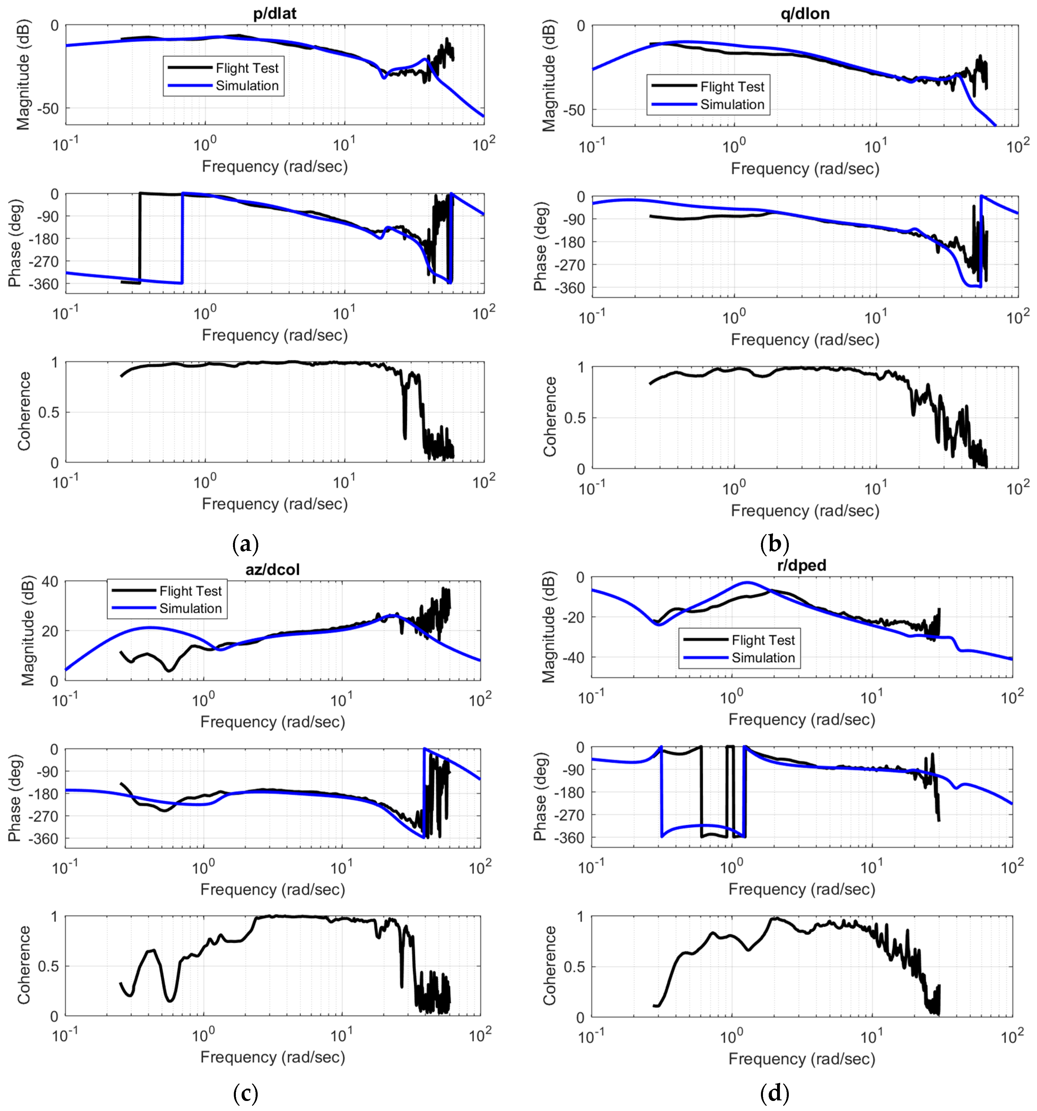
Figure 3 show sample on-axis frequency responses. The flight test frequency sweeps were processed using CIFER^® to yield frequency responses (shown in black). The coherence shows the quality of the data and the suitability of a linear transfer function representation of the dynamics. The flight test data provides reasonable frequency response between 0.7 and 30 rad/s. The blue line shows the linearized simulation model for the same frequency responses. There is good correlation across the frequencies where the coherence is high.

Figure 4 and Figure 5 show sample time history responses for 2-3-1-1 inputs in a flight test (in black) and the equivalent responses from the non-linear simulation model in blue. The control input time histories on the left were replayed into the simulation model as perturbations from the trim inceptor positions. The on-axis responses are seen to be very accurate for the first several seconds of the time history (over time the responses diverge due to instability of the aircraft dynamics). Furthermore, even the agreement of the off-axis responses is reasonable (which is notoriously difficult to model for rotorcraft).

3.4. Dynamic Inversion Controller Implementation for the Utility Helicopter Simulation

The controller is designed to achieve a rate command/attitude hold (RCAH) response in roll and pitch, and a rate command response in yaw, and vertical speed command response in the vertical axis. The final controller implementation is non-linear, in that the F(x) and G(x) functions include the non-linear kinematics and inertial coupling terms of the 6-DOF equations of motion, while the aerodynamic force terms are represented by linearized perturbation models (i.e., stability and control derivatives) for the nominal operating point (which is defined by airspeed). The stability and control derivatives are extracted directly from the reduced order linear model (as derived in Equation (25)), and scheduled with airspeed. Thus, the linearized model analysis above is simply based on a linearization of the non-linear controller, where CA and CB are Jacobian matrices of F(x) and G(x) evaluated at the trim conditions. The details of the non-linear implementation are described in earlier publications [9].

To achieve the desired rate command response types, the controlled variables (CVs) are selected as the time rate of change of the pitch and roll attitudes, the climb rate, and the body axis yaw rate.

$$y=\left[\begin{array}{c}\dot{\varphi }\\ \dot{\theta }\\ V_z\\ r\end{array}\right]=CVs$$

(31)

The roll and pitch attitude rates are controlled by lateral and longitudinal deflections of the cyclic stick, and the vertical speed by displacement of the collective stick. In hover and low speed, yaw rate is proportional to the pedal input, while in forward flight, turn coordination is achieved via a computed yaw rate as follows:

$$r_{cmd}=\frac{a_{y_{cmd}}+g\sin \varphi \cos \theta }{V}$$

(32)

where the lateral acceleration command is proportional to the pedal input.

All controlled variable commands pass through a command filter between the inceptor and the reference command. As discussed above the controlled variables in the pitch and roll axes are the attitude rates. However, the same feedback compensation formulation can be used to achieve attitude command/attitude hold (ACAH) response type (as shown in [9]) or even other response types, with slight modification to the command filter. Figure 6 shows sample command filters in the pitch axis for both RCAH and ACAH response type. For the ACAH command filter, the CV is still selected as attitude rate. The filter generates consistent reference signals for attitude, attitude rate, and attitude accelerations just as it does for the RCAH filter. The proportional integral + double integrator compensation used in the RCAH system is exactly equivalent to proportional integral derivative (PID) compensation for ACAH system. Alternatively, one could select attitudes as the CVs in the DI formulation. In that case, one finds that the control does not appear explicitly in the differentiated output and G(x) is not invertible. This requires a 2nd differentiation of the output equation (this formulation is shown in [9]). Retaining the rate as the CV results in cleaner, but equivalent formulation. The command filter structure below also allows the response type to be easily changed for different control modes, while using the same CV feedback compensation.

Since rate responses are used in each axis, the command filters are all first order associated with a natural frequency parameter. The can be selected to achieve desired response to pilot input as dictated by handling qualities specifications, e.g., ADS-33E-PRF specifications for Level 1 rotorcraft flying qualities [21]. Note that the natural frequency for the response can be different for the natural frequency used for gain selection (as shown in Equation (9)), although the two parameters might be assumed to be of similar magnitude. The command filter frequencies govern the response bandwidths in each axis, and the natural frequencies of the error dynamics in Equation (9), are used to govern disturbance rejection bandwidth. If the aircraft follows the rate command response perfectly, the response bandwidth based on phase margin (as defined in ADS-33E-PRF) will be identical to the command filter natural frequency. In practice, the bandwidth will be slightly lower due to phase roll off of the full order dynamics. According to the idealized analysis of Equation (9), the error dynamics can be specified by any three poles through proper gain selection. In reality, because of discrepancies between the reduced order linear model and the true dynamics, there are stability constraints on the gains. As shown in [10], gain selection becomes a design tradeoff between disturbance rejection and robust stability, as will be illustrated in Section 4.1. The nominal parameters for the DI design are listed in

Table 1. Summary of command filter and feedback gain parameters for nominal controller design.

Control Axis	Command Filter Frequency	Error Dynamics Parameters
Roll	${\omega }_n=2.6\mathrm{rad}/\mathrm{s}$	$\begin{array}{c}{\omega }_n=2.0\mathrm{rad}/\mathrm{s}\\ \zeta =1.0p=0.4\end{array}$
Pitch	${\omega }_n=2.1\mathrm{rad}/\mathrm{s}$	$\begin{array}{c}{\omega }_n=2.0\mathrm{rad}/\mathrm{s}\\ \zeta =1.0p=0.4\end{array}$
Heave	${\omega }_n=0.5\mathrm{rad}/\mathrm{s}$	$\begin{array}{c}{\omega }_n=0.5\mathrm{rad}/\mathrm{s}\\ \zeta =1.0p=0\end{array}$
Yaw	${\omega }_n=3.6\mathrm{rad}/\mathrm{s}$	$\begin{array}{c}{\omega }_n=2.5\mathrm{rad}/\mathrm{s}\\ \zeta =1.0p=0\end{array}$

below. The roll, pitch, and yaw command filter frequencies are designed to meet the bandwidth requirements for target acquisition and tracking in forward flight with a design margin of 0.1 rad/s. These do not address the phase delay requirement, which would also have to be checked. The heave-axis frequency is designed to achieve the required time constant for height and flight path response.

4. Results

The stability and performance of the DI controller were investigated using the validated simulation of the utility helicopter. A linear systems analysis was used to study the closed-loop stability of the system and the impact of NMP zeros. Stability margins versus disturbance rejection bandwidth properties were studied to understand tradeoffs between stability robustness and disturbance rejection performance. In addition, non-linear simulations are conducted to view command tracking performance and to verify the linear model analyses.

4.1. Linear Analysis

An analysis of the linearized dynamics (both open-loop and closed-loop) was conducted to demonstrate the stability and performance of the DI control design. Analysis is focused on the 80 kts flight condition as presented in the validation Section 3.3. The open loop system dynamics (as modelled by the full and reduced order models) are illustrated in Figure 7, which shows the eigenvalues and transmission zeros of the MIMO system (from inputs to controlled variable outputs). The figure on the right shows a close up of the low-frequency poles and zeros associated with the rigid body dynamics. The poles (eigenvalues) are summarized in

Table 2. Summary of eigenvalues at 80 kts forward flight, full and reduced order models.

Mode	Full Order Eigenvalues	Reduced Order Eigenvalues
Spiral	−0.0627	−0.0627
Phugoid	0.0977 ± 0.433i	0.100 + 0.435i
Dutch Roll	−0.374 ± 1.22i	−0.373 + 1.228i
Coupled Roll/Pitch Short Period	−3.019 ± 1.64i	−2.80 + 0.746i
Coupled Roll/Pitch Short Period	−0.512	−0.526
Roll/Regressing Flap	−6.622
Differential Lead/Lag	−3.20 ± 6.93i
Inflow Skew Distortion Mode	−7.96
Regressing Flap	−13.1 ± 4.28i
Collective Lead/Lag	−13.8 ± 12.4i
Regressing Lead/Lag	−2.33 ± 18.1i
Coning Mode	−7.85 ± 22.8i
Differential Flap	−13.9 ± 22.5i
Cyclic Inflow	−37.4 ± 9.65i
Progressing Lead/Lag	−3.23 ± 38.7i
Blade Twist Mode	−46.6
Tail Rotor Inflow Mode	−53.1
Progressing Flap	−12.4 ± 48.8i

, which identifies the modes based on analysis of the eigenvectors, and the transmission zeros are shown in

Table 3. Summary of transmission zeros at 80 kts forward flight, full and reduced order models, and along with eigenvalues of with feedback linearization loop closed. The underlined values indicate NMP zeros and corresponding unstable eigenvalues in the closed loop system.

Zeros of Full Order Open Loop System	Zeros of Reduced Order Open Loop System	Eigenvalues of Full Order System with Approximate Feedback Linearization	Eigenvalues of Reduced Order System with Feedback Linearization	Zeros of Reduced Order System with Output Redefinition
0	0	0	0	0
0	0	0	0	−0.0536 ± 0.591i
0.0283	0.0283	0	0	−0.0788
−0.0788	−0.0788	0	0
−7.48		0	0
−10.1		0	0
−2.76 ± 7.35i		0.123	0.0283
−13.6 ± 11.8i		−0.0399 ± 0.173i	−0.0788
−11.9 ± 15.5i		−0.166
−20.3		−6.17
−0.675 ± 17.8i		−3.15 ± 7.25i
−31.9		−15.1 ± 5.29i
−36.9		−13.8 ± 12.4i
−29.9 ± 19.1i		−7.59
−7.32 ± 47.3i		−2.12 ± 18.4i
−62.9		−8.51 ± 22.5i
77.2		−13.6 ± 21.8i
−116.		−37.4 ± 9.32i
107. ± 17.4i		−4.23 ± 39.6i
		−46.4
		−52.7
		−12.9 ± 49.0i

.

The analysis shows that the reduced order model is indeed a good approximation of the low frequency dynamics of the aircraft. Furthermore, the high order model has a number of high-frequency zeros, which would be problematic if one applied feedback linearization on the full order system. Those zeros would result in quickly divergent unstable modes of the closed loop system. The reduced order model has one very low frequency zero, which would result in a low-frequency instability.

Now the feedback linearization loop is applied to the full- and reduced-order systems with no controlled variable feedback (K(s) = 0). For the reduced order model, we have perfect inversion, and indeed there are four zero eigenvalues, and four eigenvalues identical to the zeros of the reduced order model. For the full-order system with approximate feedback linearization, there are still four zero eigenvalues, as well as four eigenvalues slightly different from the zeros for the reduced order model. In addition, there are several stable high frequency modes.

Note that the unstable eigenvalue increases with application of feedback linearization to the full-order mode, but there are no large magnitude, unstable eigenvalues corresponding to the large NMP zeros of the full-order system. The eigenvalue at 0.123 is in fact manageable; its value is reduced with CV feedback and then can be stabilized with outer loop control or pilot compensation. Application of this model results in a slow airspeed instability. A physical explanation is that if one constrains the pitch attitude of the rotorcraft, it will have no tendency to return to the trim airspeed. For the purpose of this study, the mode will be handled through output redefinition. A small component of forward speed is added to the pitch axis CV

$$y=\left[\begin{array}{c}\dot{\varphi }\\ \dot{\theta }-0.01u\\ V_z\\ r\end{array}\right]=CVs$$

(33)

The change in CV results in stable closed loop dynamics. In practice, the forward speed measurement is sent through a high-pass filter to avoid issue of defining perturbation from trim airspeed.

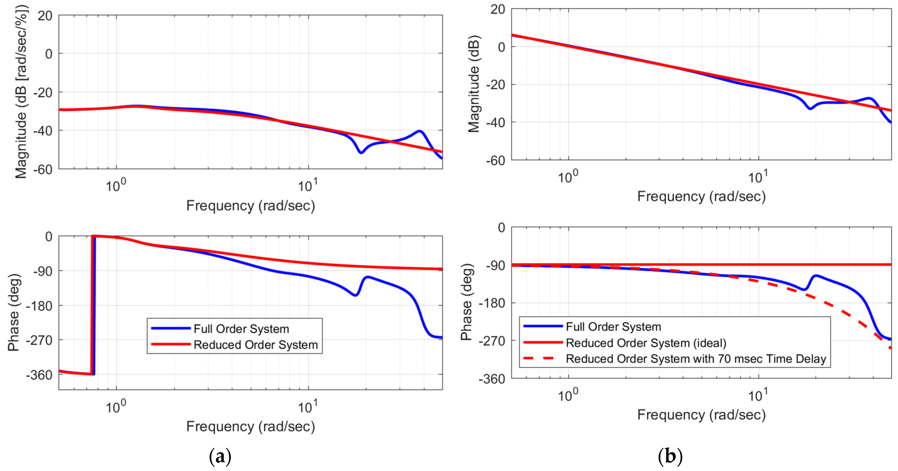
Figure 8 shows sample roll-axis frequency responses of the open loop systems and the full- and reduced-order systems with feedback linearization. As expected, the reduced order model shows perfect conversion to integrator dynamics. The full-order system approximates an integrator with and added time delay (estimated as 70 ms). Thus, when we apply controlled variable feedback to the full-order system we expect some added phase lag and reduced stability margin relative to the case of ideal feedback linearization.

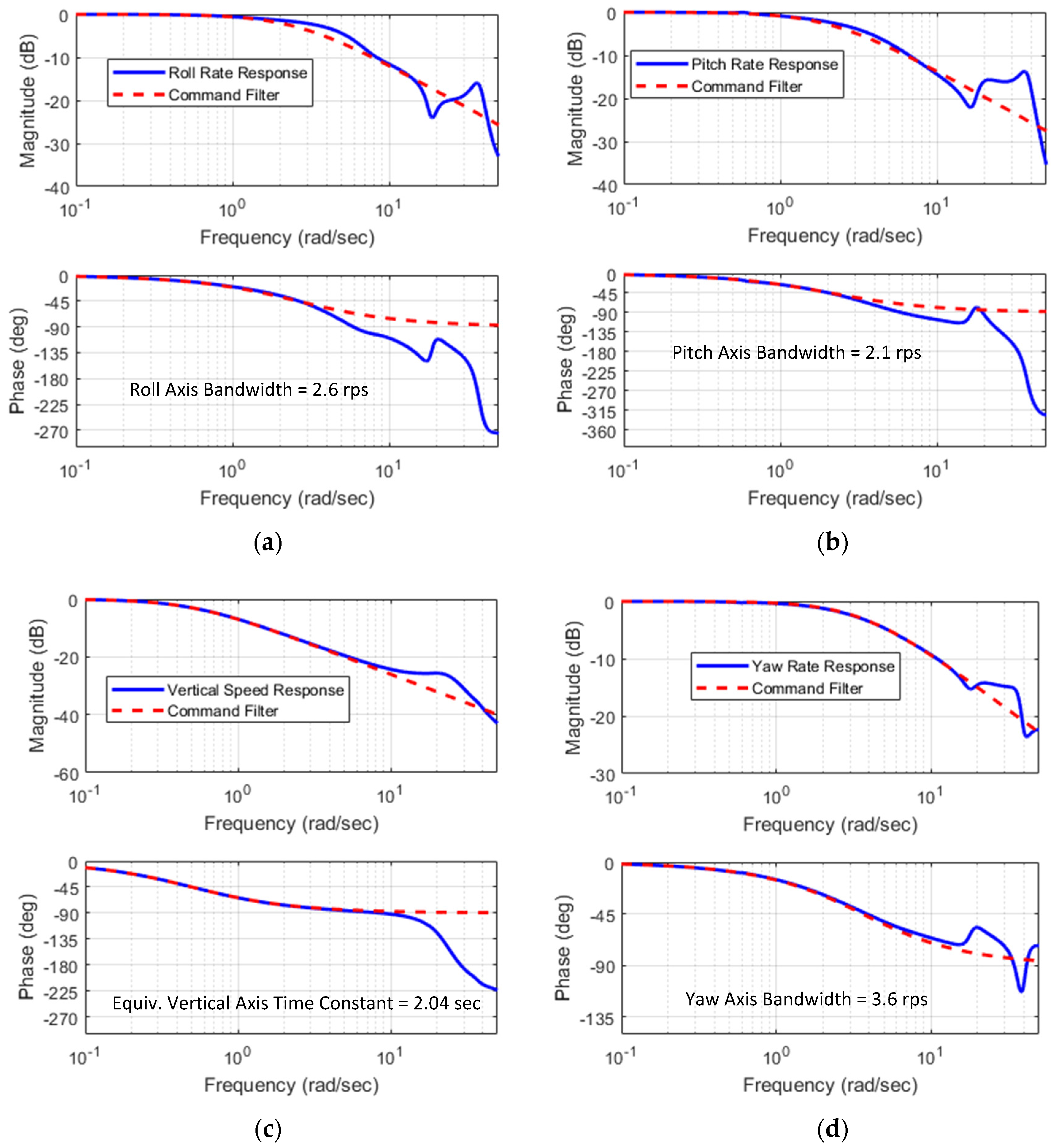
CV feedback is applied in the form of proportional + integral + double integral (PII) feedback for roll and pitch rates, and PI feedback for vertical speed and yaw using the nominal gains described in Table 1. Figure 9 shows sample closed-loop bode plots from each commanded CV to the response of the corresponding CV. The ideal command filter is also shown for reference (when using the reduced order plant model, the analysis shows this response is followed perfectly).

Note that ADS-33F defines the phase margin bandwidth as the frequency where phase of the attitude response to pilot input passes through −135°. Since these plots are for the attitude rates, the bandwidth is seen as the crossing of −45° (since attitudes are a pure integration of the rates). Attitude frequency responses were also evaluated to ensure that the gain margin bandwidth was not less than the phase margin bandwidth and to evaluate the equivalent phase delays. The resulting bandwidth values from roll, pitch, and yaw matched the command filter design natural frequency in Table 1 within two significant figures. The vertical axis frequency response is first order up to 10 rad/s with a break frequency 0.49 rad/s. This also matched the design natural frequency and resulted in equivalent time constant of 2.04 s (which corresponds to Level I vertical response for ADS-33E-PRF).

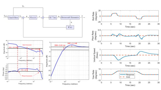
The feedback design is based on a tradeoff of stability margins and disturbance rejection of the controller [10,22,23]. Stability margins were evaluated by extracting linear models of the open loop plant due to a disturbance at each actuator, as is standard practice for flight control design on piloted military aircraft [24]. The analysis considers single-axis loop breaks, and extracts the linear model from the actuator to the loop break, as shown in Figure 10a. The disturbance rejection bandwidth (DRB) was evaluated by analyzing the closed-loop linear model from a disturbance at the plant output to the corresponding output as shown in Figure 10b. The outputs of interest for each axis are those of the hold feature of the controller: roll attitude, pitch attitude, altitude, and heading. The resulting system is a zero DC gain transfer function, as was shown in Equation (9) for the perfect inversion. The full order dynamics produce a much higher order zero DC gain system, and the frequency at which the magnitude crosses −3 dB is defined as the DRB. As described in [22], this provides a measure of the disturbance rejection performance of the hold modes of the controller by defining the frequency below which external disturbances are effectively rejected. In addition, the disturbance rejection peak (DRP) is defined as the peak amplitude of the frequency response. This provides measure of the system damping or tendency to overshoot responding to disturbances.

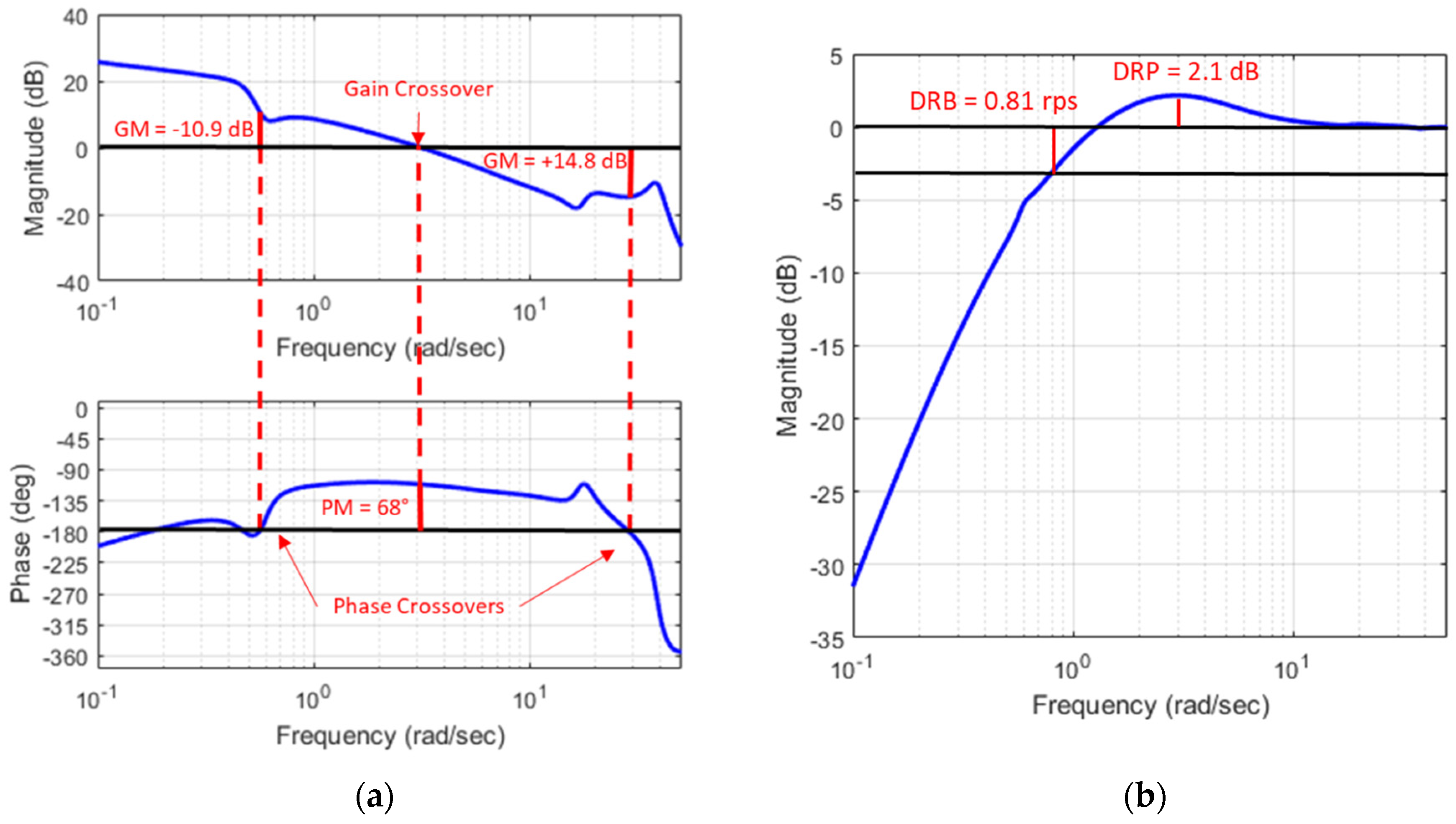
Note that the DRB analysis provides a single input/single output (SISO) variant of the sensitivity function commonly used in robust control theory for MIMO systems. The stability margin analysis is a SISO analysis of robustness, similar to small gain theory used in MIMO robust control theory but with the added measure of robustness to phase delay. The SISO analysis is appropriate due to the decoupling achieved by the DI inner loop, as will be illustrated in the gain optimization. Figure 11 shows sample frequency responses used in stability margin (SM) and DRB/DRP analyses for the pitch axis with the nominal controller gains.

Figure 11 shows sufficiently high gain and phase margins in the pitch axis. Standard design practice requires 6 dB gain margin (GM) and 45° of phase margin (PM) [24], and thus the stability analysis implies there is significant design space to increase gains and optimize the disturbance rejection performance of the pitch axis controller. This is in fact true of all four control axes.

Now a gain optimization study is performed to maximize disturbance rejection performance of the aircraft while maintaining constraints on stability margins and the disturbance rejection peak. As discussed above, control design guidelines require 6 dB gain margin and 45° phase margin. In addition, the time delay margin (DM) can also be evaluated as phase margin divided by the gain crossover frequency. A design can have good phase margin, but with high gain crossover the time delay margin can be unacceptably low. For this design, we set a DM constraint of 100 ms. For disturbance rejection, recent studies have proposed minimum DRB values for each axis, and a maximum DRP of 5 dB [25]. The recommended Level 1 DRB values are 0.8 rad/s for roll attitude hold, 0.5 rad/s in pitch attitude hold, 0.7 rad/s in yaw attitude hold, and 0.17 rad/s for altitude hold. The nominal design meets all of these requirements. However, disturbance rejection can be considered a performance objective that can be optimized in order to minimize tracking errors due to both modeling error and disturbances.

For brevity, only the pitch axis gain optimization will be presented.

Table 4. Variation in pitch axis stability margins and disturbance rejection performance with variation in pitch axis gain parameters.

Error Dynamics Parameters for Pitch Gain Selection (rad/s)	Gain Margin (dB)	Phase Margin (deg)	Delay Margin (ms)	Gain Crossover (rad/s)	DRB (rad/s)	DRP (dB)
${\omega }_n=2.0\zeta =1.0p=0.4$	14.8	68.7	384	3.12	0.814	2.17
${\omega }_n=3.0\zeta =1.0p=0.6$	9.97	56.6	194	5.07	1.24	2.41
${\omega }_n=4.0\zeta =1.0p=0.8$	6.56	51.2	132	6.77	1.66	2.63
${\omega }_n=5.0\zeta =1.0p=1.0$	4.01	47.7	98.6	8.44	2.08	2.82
${\omega }_n=6.0\zeta =1.0p=1.2$	2.00	44.2	76.3	10.1	2.51	2.99
${\omega }_n=7.0\zeta =1.0p=1.4$	0.313	40.5	60.9	11.6	2.93	14.0

shows the variation in stability margins, DRB, and DRP with increases in the natural frequency of the pitch axis error dynamics. As discussed in Equation (9), this parameter is used for feedback gain selection. The real pole is set at one fifth of the natural frequency, and the damping ratio fixed at 1.0. The table shows the expected trend of decreasing stability margins and increasing disturbance rejection bandwidth as the gains are increased. Above natural frequency 4.0, the gain margin is below design requirements, and the delay margin drops below 100 ms. At ω_n = 7.0 rad/s, the gain margin is very small, and in fact the controller becomes unstable around ω_n = 7.3 rad/s.

Table 5. Variation in roll axis stability margins and disturbance rejection performance with variation in pitch axis gain parameters.

Error Dynamics Parameters for Pitch Gain Selection (rad/s)	Gain Margin (dB)	Phase Margin (deg)	Delay Margin (ms)	Gain Crossover (rad/s)	DRB (rad/s)	DRP (dB)
${\omega }_n=2.0\zeta =1.0p=0.4$	25.7	69.6	771	1.58	0.834	2.18
${\omega }_n=3.0\zeta =1.0p=0.6$	24.5	69.7	770	1.58	0.834	2.19
${\omega }_n=4.0\zeta =1.0p=0.8$	22.9	69.8	771	1.58	0.834	2.19
${\omega }_n=5.0\zeta =1.0p=1.0$	20.4	69.9	772	1.58	0.834	2.19
${\omega }_n=6.0\zeta =1.0p=1.2$	16.4	69.9	772	1.58	0.834	2.19
${\omega }_n=7.0\zeta =1.0p=1.4$	6.33	69.9	772	1.58	0.834	2.19

shows the behavior of the roll axis with variation in the pitch axis gains. The roll axis gains, as well as the other two axes, are fixed at the nominal values set by Table 1. The table, therefore, shows the behavior of different axes to gain variation in pitch. With the exception of the gain margin, stability and performance of the roll axis virtually unaffected by the pitch axis gain variation. The same is true for the yaw and vertical axes. Gain margin decreases, but is generally well above the design requirement, until the closed-loop system becomes nearly unstable, at which all gain margins approach 0. The results show the effective de-coupling of the DI control scheme.

The gain optimization was performed independently for each axis, varying single axis gains while holding the gains for the other axes at their nominal value. The final gain parameters were then applied to all axes, and the performance was evaluated. Some additional tuning was required as the gain margins degraded slightly with increased gain in multiple axes (compared to the single axis gain optimization). On the other hand, individual axis tuning was a good predictor of the final phase margins and DRB. The final parameters and the performance are summarized in

Table 6. Final controller performance with selected gains. The underlined parameters indicate the parameter that limits the gain used in each axis.

Error Dynamics Parameters for Pitch Gain Selection (rad/s)	Gain Margin (dB)	Phase Margin (deg)	Delay Margin (ms)	Gain Crossover (rad/s)	DRB (rad/s)	DRP (dB)
Roll Axis ${\omega }_n=4.2\zeta =1.0p=0.84$	6.38	56.8	159	6.24	1.73	3.02
Pitch Axis ${\omega }_n=3.3\zeta =1.0p=0.66$	6.38	57.1	170	5.86	1.40	2.62
Vertical Axis ${\omega }_n=1.0\zeta =1.0p=0.0$	24.4	75.2	103	1.27	0.404	1.26
Yaw Axis ${\omega }_n=4.5\zeta =1.0p=0.0$	∞	83.9	157	9.30	1.81	1.17

. The underlined margin indicates the critical stability margin for that axis, with the exception of the yaw axis where the gain crossover was constrained to less than 10 rad/s. Higher crossovers would likely cause problems with actuators or structural modes. If structural modes were included in the model, the yaw axis crossover would probably need to be reduced even further.

4.2. Time Response of Non-Linear Simulation

The controller was tested in the complete non-linear simulation, PSUHeloSim, with the non-linear controller. Figure 12 shows time history response of a 30° banked turn maneuver at 80 kts. The maneuver is achieved by a 10 deg/s roll rate pulse command to the right followed 10 s later by an equal magnitude pulse to left. The turn coordination logic in the yaw axis (Equation (32)) produces the yaw rate command for a coordinated turn. The figure shows the controller tracks the reference model commands very well, with root-mean-squared (RMS) tracking error of 0.120 deg/s, 0.0676 deg/s, and 0.0561 deg/s in roll, pitch, and yaw respectively. The tracking error in vertical speed is 0.344 ft/s. The actuator activity is also shown along with the attitude, airspeed, and altitude time histories.

To illustrate the performance of the controller across a range of operating conditions, the same maneuver was repeated at airspeeds of 60 kts, 100 kts, 120 kts, and 140 kts. The RMS tracking errors were evaluated for each case and are summarized in

Table 7. RMS tracking errors of at various airspeeds for a 30° banked turn maneuver.

Airspeed (kts)	Roll Rate RMS Tracking Error (deg/s)	Pitch Rate RMS Tracking Error (deg/s)	Vertical Speed RMS Tracking Error (ft/s)	Yaw Rate RMS Tracking Error (deg/s)
60	0.120	0.0843	0.0601	0.328
80	0.120	0.0676	0.0561	0.344
100	0.123	0.0636	0.0512	0.361
120	0.135	0.0721	0.0535	0.317
140	0.190	0.0826	0.0849	0.0302

. The results show very consistent performance for every airspeed (with some mild degradation at 140 kts), even though the feedback gains are exactly the same for each case. The results show the reduced reliance on gain scheduling when using NDI. A rigorous design would still perform stability margin analysis at every condition and possibly schedule gains to meet desired margins, but the method simplifies design since it effectively separates the command tracking performance and stability analysis.

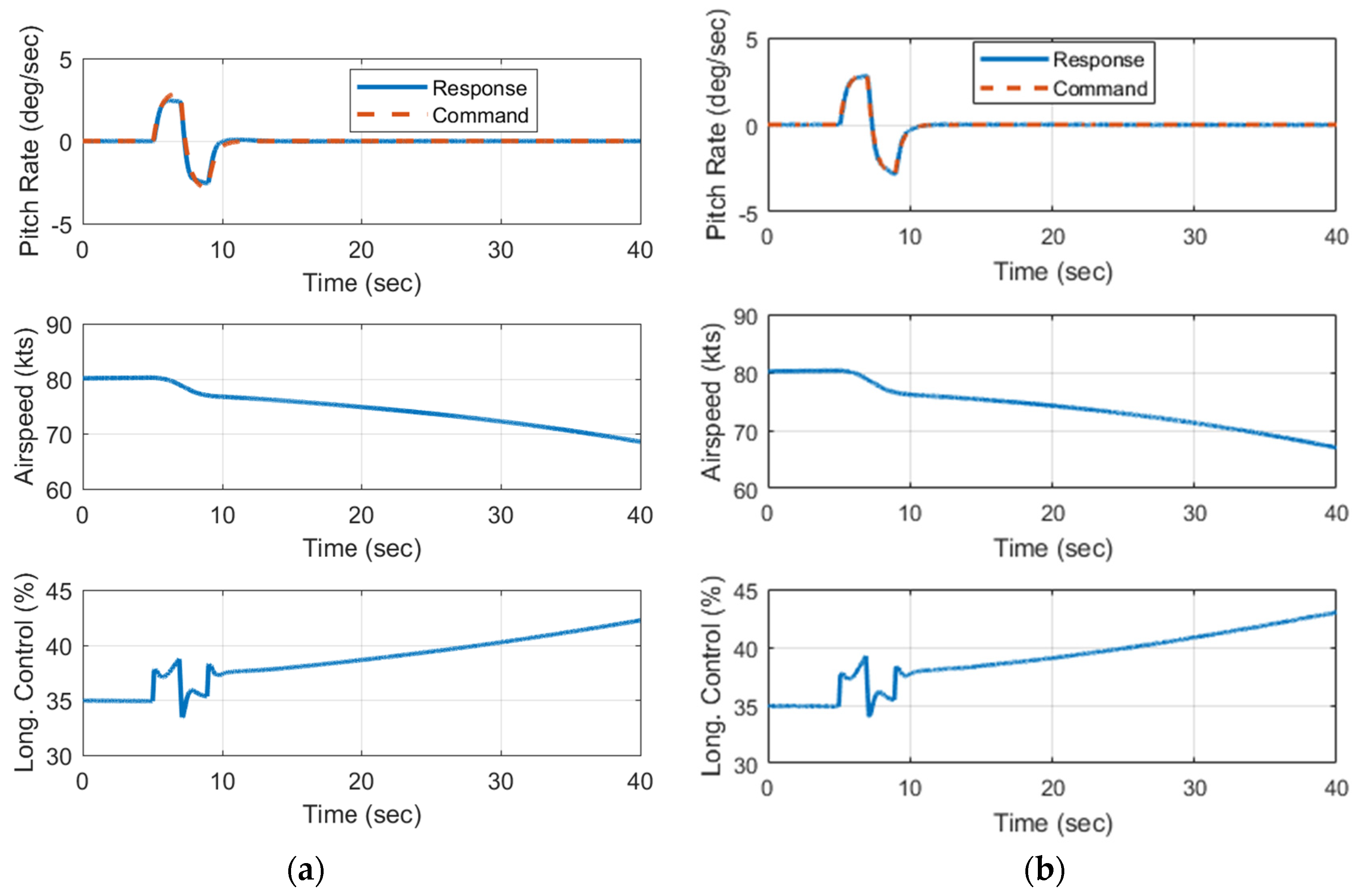
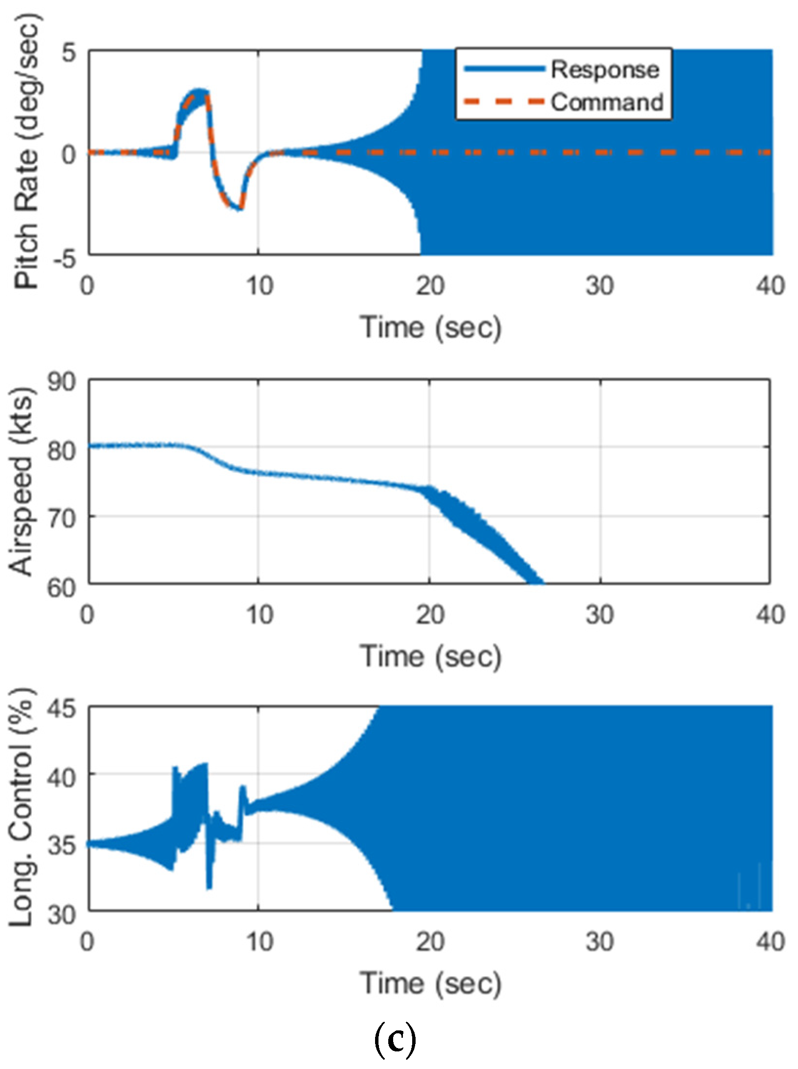
As noted in the derivation, two potential pitfalls in DI design are NMP zeros, and excessive CV feedback gain causing instability due to the high order dynamics. In the control development an output redefinition scheme was applied to address NMP zeros. Figure 13a shows response due to a pitch rate doublet with the final controller design. The tracking is reasonably good, but a slow divergence of the airspeed is observed. In Figure 13b, the output redefinition is removed such that the pitch axis CV is simply pitch attitude rate, and the same maneuver was simulated. The results show that the rate of airspeed divergence is slightly increased, but the attitude rate tracking is actually improved. The results tend to indicate that the output redefinition method was not successful, and that the best method to handle the NMP zero and unstable airspeed mode is with an outer loop controller. Finally, Figure 13c shows the result of excessive feedback gain in the pitch axis. The natural frequency parameter for the pitch axis was increased in 0.2 rad/s increments and the corresponding gains recalculated. The pitch doublet maneuver was repeated until instability was observed. This occurred when ω_n = 6.8 rad/sec, slightly lower than the value predicted by linear analysis (ω_n = 7.3 rad/s). The result indicates the need for some conservativeness when choosing gains and final stability margins, but generally the analysis was effective.

5. Discussion

The application of dynamic inversion (DI) to rotorcraft flight control design was investigated. A DI design procedure was developed and demonstrated with a validated simulation of a utility helicopter.

There are two primary challenges in designing a DI controller for rotorcraft: (1) the input–output dynamics from actuators to the controlled variables will often have NMP zeros, and in fact this is inevitable when one considers the full order system with rotor dynamics. (2) The requirement of full state feedback is not feasible when considering the complete dynamics of the rotorcraft due to the excessive cost of instrumentation required to measure (or accurately estimate) the rotor and inflow states. The proposed solution to both of these issues is the use of reduced order models. The reduced order models represent the low-frequency dynamics of the rotorcraft by assuming fast dynamics are stable and quickly reach steady-state (based on the principles of singular perturbation theory). The reduced order state vector consists of rigid body states of the rotorcraft, which are readily measured and/or estimated. In addition, it is shown that the-high frequency NMP zeros are removed via the order reduction method, while low-frequency NMP zeros are handled by output redefinition or outer loop control.

The results of the DI design found that the reduced order model is indeed a good low frequency model of the utility helicopter. The feedback linearization converts the plant model to a system resembling a set of de-coupled integrators with an added phase delay up to a frequency of 10–20 rad/s. CV feedback stabilizes the system (according to linear analysis), and results in good tracking of CV variable commands. A key aspect of the design method is to check relative stability and controller performance against the full-order linear dynamics to verify desired stability margins via classical gain margin, phase margin, and time delay margin analysis. The analysis demonstrated that the decoupled nature of the dynamics after feedback linearization justifies these well-established SISO methods of determining relative stability.

Non-linear simulations showed that the final NDI design performed well in tracking commands. However, speed instability could be observed for a pitch doublet perturbation showing that the output redefinition approach did not fully address the issue of NMP zeros. However, the speed divergence was very slow and could readily be stabilized with outer loop control. Furthermore, analysis showed that the gain limit for the pitch axis determined by linear gain margin analysis was a reasonable estimate of the true gain limit observed when testing in non-linear simulation.

Overall, the DI design method appears to be a feasible control solution for rotorcraft. It is notable that the same issues of NMP zeros arise with EMF design. Handling NMP zeros is tractable for both design methods. The DI design has some advantages in that the number of NMP zeros is reduced to those of a single MIMO system rather than several individual SISO transfer functions. Furthermore, DI has the advantage that the need for gain scheduling is minimized since the feedback design is applied around the de-coupled linearized system, and gain optimization can readily be treated as a SISO design problem. This was illustrated by the simulations showing very consistent performance of the controller across a range of airspeeds, without any variation in gains. A more comprehensive design might perform a multi-variable optimization of the gains for each operating point, but that optimization might be simplified due to the de-coupled nature of the system after feedback linearization.

References

- Tischler, M.B.; Remple, R.K. Chapter 1.3. Special Challenges of Rotorcraft System Identification. In Aircraft and Rotorcraft System Identification: Engineering Methods with Flight Test Examples, 2nd ed.; American Institute of Aeronautics and Astronautics: Reston, VA, USA, 2012; pp. 10–11. [Google Scholar]
- Key, D. Analysis of Army Helicopter Pilot Error Mishap Data and the Implications for Handling Qualities. In Proceedings of the 25th European Rotorcraft Forum, Rome, Italy, 14–16 September 1999. [Google Scholar]
- Harding, J.; Moody, S.J.; Jeram, G.J.; Mansur, M.H.; Tischler, M.B. Development of Modern Control Laws for the AH-64D in Hover/Low Speed Flight. In Proceedings of the 62nd Annual Forum of the American Helicopter Society, Phoenix, AZ, USA, 9–11 May 2006. [Google Scholar]
- Whalley, M.; Howitt, J. Optimization of Partial Authority Automatic Flight Control Systems for Hover Low-Speed Maneuvering in Degraded Visual Environments. J. Am. Helicopter Soc. 2002, 47, 79–89. [Google Scholar] [CrossRef]
- Bender, J.; Irwin, J.G.; Spano, M.S.; Schwerke, M. MH-47G Digital AFCS Evolution. In Proceedings of the 67th Annual Forum of the American Helicopter Society, Virginia Beach, VA, USA, 3–5 May 2011. [Google Scholar]
- Enns, D.; Bugaski, R.H.; Stein, G. Dynamic inversion: An evolving methodology for flight control design. Int. J. Control 1994, 59, 71–91. [Google Scholar] [CrossRef]
- Harris, J.J.; Stanford, J.R. F-35 Flight Control Law Design, Development and Verification. In Proceedings of the 2018 Aviation Technology, Integration, and Operations Conference, AIAA AVIATION Forum, Atlanta, GA, USA, 25–29 June 2018. [Google Scholar] [CrossRef]
- Jacubczyk, B.; Respondek, W. On Linearization of Control Systems. Bulliten Academie Polonaise de Science et Mathematique 1980, 28, 517–522. [Google Scholar]
- Soneson, G.L.; Horn, J.F.; Zheng, A. Simulation Testing of Advanced Response Types for Ship-Based Rotorcraft. J. Am. Helicopter Soc. 2016, 61, 1–13. [Google Scholar] [CrossRef]
- Horn, J.F.; Yang, J.; He, C.; Lee, D. Parameter Optimization of Dynamic Inversion Control Laws for Shipboard Operations. In Proceedings of the 73rd AHS Annual Forum, Fort Worth, TX, USA, 9–11 May 2017. [Google Scholar]
- Stevens, B.L.; Lewis, F.L.; Johnson, E.N. Aircraft Control and Simulation: Dynamics, Controls Design, and Autonomous Systems, 3rd ed.; John Wiley & Sons: Hoboken, NJ, USA, 2016; Chapter 5.8. [Google Scholar]
- Catapang, D.R.; Tischler, M.B.; Biezad, D.J. Robust Crossfeed Design for Hovering Rotorcraft. Int. J. Robust Nonlinear Control 1994, 4, 161–180. [Google Scholar] [CrossRef]
- Spires, J.M.; Horn, J.F. Multi-Input Multi-Output Model-Following Control Design Methods for Rotorcraft. In Proceedings of the American Helicopter Society 71st Annual Forum, Virginia Beach, VA, USA, 5–7 May 2015. [Google Scholar]
- Hovakimyan, N.; Lavretsky, E.; Cao, C. Dynamic inversion for multivariable non-affine-in-control systems via time-scale separation. Int. J. Control 2008, 81, 1960–1967. [Google Scholar] [CrossRef]
- Oppenheimer, M.W.; Doman, D.B. Control of an Unstable, Non-minimum Phase Hypersonic Vehicle. In Proceedings of the 2006 IEEE Aerospace Conference, Big Sky, MT, USA, 4–11 March 2006. [Google Scholar]
- Ryu, J.H.; Park, C.S.; Tahk, M.J. Plant Inversion Control of Tail Controlled Missile. In Proceedings of the AIAA Guidance, Navigation, and Control Conference, New Orleans, LA, USA, 11–13 August 1997. [Google Scholar]
- Howlett, J. UH60A BLACK HAWK Engineering Simulation Program: Volume I Mathematical Model; NASA CR166309; National Aeronautics and Space Administration: Washington, WA, USA, 1981. [Google Scholar]
- Zhao, J. Dynamic Wake Distortion Model for Helicopter Maneuvering Flight. Ph.D. Thesis, Georgia Institute of Technology, Atlanta, GA, USA, March 2005. [Google Scholar]
- Fletcher, J. A Model Structure for Identification of Linear Models of the UH-60 Helicopter in Hover and Forward Flight; NASA TM 110362; NASA Ames Research Center: Moffett Field, CA, USA, 1995. [Google Scholar]
- Cauffman, M.G.; Tischler, M.B. Frequency-Response Method for Rotorcraft System Identification: Flight Applications to BO 105 Coupled Rotor/Fuselage Dynamics. J. Am. Helicopter Soc. 1992, 37, 3–17. [Google Scholar]
- Baskett, B.J. Aeronautical Design Standard, Performance Specification, Handling Qualities Requirements for Military Rotorcraft; ADS-33E-PRF; US Army Aviation and Missile Command: Redstone Arsenal, AL, USA, 2000.
- Mansur, M.H.; Lusardi, J.A.; Tischler, M.B.; Berger, T. Achieving the Best Compromise between Stability Margins and Disturbance Rejection Performance. In Proceedings of the American Helicopter Society 65th Annual Forum, Grapevine, TX, USA, 27–29 May 2009. [Google Scholar]
- Zheng, A.; Horn, J.F. Investigation of Bandwidth and Disturbance Rejection Properties of a Dynamic Inversion Control Law for Ship-Based Rotorcraft. In Proceedings of the American Helicopter Society 71st Annual Forum, Virginia Beach, VA, USA, 5–7 May 2015. [Google Scholar]
- Anon. Flight Control Systems—Design, Installation, and Test of Piloted Military Aircraft, General Specification for; SAE-AS94900; SAE International: Warrendale, PA, USA, July 2007. [Google Scholar]
- Blanken, C.L.; Tischler, M.B.; Lusardi, J.A.; Ivler, C.M. Aeronautical Design Standard-33 (ADS-33) ... Past, Present and Future. In Proceedings of the American Helicopter Society Rotorcraft Handling Qualities Specialists’ Meeting, Huntsville, AL, USA, 22–23 February 2014. [Google Scholar]
Figure 1.
Schematic of dynamic inversion (DI) flight control architecture.
Figure 2.
Simplified single-input single-output (SISO) dynamics following ideal feedback linearization.
Figure 3.
On-axis frequency responses from flight test [19] and the simulation model at 80 kts forward airspeed, showing good correlation from 0.7 to 30 rad/s, (a) roll rate due to lateral cyclic input; (b) pitch rate due to longitudinal cyclic input; (c) vertical acceleration due to collective input; (d) yaw rate response due to pedal input.
Figure 4.
Sample time domain response of 2-3-1-1 lateral input from flight test [19] and the simulation model at 80 kts forward airspeed.
Figure 5.
Sample time domain response of 2-3-1-1 longitudinal input from flight test [19] and the simulation model at 80 kts forward airspeed.
Figure 6.
Structure of command filters for (a) rate command attitude hold, and (b) attitude command attitude hold.
Figure 7.
Pole-zero map of full and reduced order dynamic models at 80 kts. (a) The full-order model exhibits three very high frequency non-minimum phase (NMP) zeros. The reduced order model poles and zeros are all clustered at low frequency, corresponding to the rigid body modes. (b) Close up at low frequency focuses on the rigid body modes and nearby zeros. Note that the reduced order model poles and zeros nearly overlay corresponding full order model poles and zeros, with the exception of the poles with real parts around −3, where there is some discrepancy in damping. The full and reduced order both have one very low frequency zero in the right half plane. As will be shown, this non-minimum phase zero will cause the controlled system to have a very slow divergent mode when using a dynamic inversion (DI) design with the reduced order model. This can be fixed through a small change in controlled variable (CV). The high frequency zeros of the full order system would be much more problematic, if one attempted to design DI with this high order model.
Figure 8.
Frequency responses of helicopter linear models at 80 kts: (a) open loop roll rate response to lateral cyclic input, full order and reduced order models; (b) response of roll rate to lateral pseudo-command with feedback linearization loop closed, full order system, reduced order system (which represents an ideal integrator response), and reduced order system with a time delay (which represents a reasonable approximation of the full order system up to 15 rad/s).
Figure 9.
Closed-loop frequency response of the helicopter model at 80 kts: (a) roll rate response to commanded roll rate; (b) pitch rate response to commanded pitch rate; (c) vertical speed response to commanded vertical speed; (d) yaw rate response to commanded yaw rate.
Figure 10.
Linear analysis diagrams for: (a) stability margin (SM) analysis with single-axis loop break; (b) disturbance rejection bandwidth (DRB) analysis with disturbance at sensor output.
Figure 11.
Sample SM and DRB analysis curves: (a) Broken loop frequency response for pitch axis for gain and phase margin analysis; (b) Sensitivity function of the pitch attitude feedback used for DRB analysis.
Figure 12.
Time history response for a 30° banked turn maneuver, (a) tracking of DI-controlled variables; (b) actuator activity; (c) attitude, airspeed, and altitude response.
Figure 13.
Time history response for a 3 deg/s pitch rate doublet: (a) with final controller design; (b) without output redefinition in the pitch axis; (c) with high pitch axis gains (error dynamic frequency ωn = 6.8 rad/s).