Flow Visualization around a Flapping-Wing Micro Air Vehicle in Free Flight Using Large-Scale PIV


1
Department of Aerospace Engineering, Delft University of Technology, 2629HS Delft, The Netherlands
2
Department of Aerospace Engineering, Middle East Technical University, 06800 Çankaya/Ankara, Turkey
*
Author to whom correspondence should be addressed.
Aerospace 2018, 5(4), 99; https://doi.org/10.3390/aerospace5040099
Submission received: 14 August 2018
/
Revised: 11 September 2018
/
Accepted: 18 September 2018
/
Published: 20 September 2018
(This article belongs to the Special Issue Bio-Inspired Aerospace System)
Abstract
:Flow visualizations have been performed on a free flying, flapping-wing micro air vehicle (MAV), using a large-scale particle image velocimetry (PIV) approach. The PIV method involves the use of helium-filled soap bubbles (HFSB) as tracer particles. HFSB scatter light with much higher intensity than regular seeding particles, comparable to that reflected off the flexible flapping wings. This enables flow field visualization to be achieved close to the flapping wings, in contrast to previous PIV experiments with regular seeding. Unlike previous tethered wind tunnel measurements, in which the vehicle is fixed relative to the measurement setup, the MAV is now flown through the measurement area. In this way, the experiment captures the flow field of the MAV in free flight, allowing the true nature of the flow representative of actual flight to be appreciated. Measurements were performed for two different orientations of the light sheet with respect to the flight direction. In the first configuration, the light sheet is parallel to the flight direction, and visualizes a streamwise plane that intersects the MAV wings at a specific spanwise position. In the second configuration, the illumination plane is normal to the flight direction, and visualizes the flow as the MAV passes through the light sheet.

1. Introduction
The development of flapping-wing micro air vehicles (MAVs) has received interest in view of their small size, relatively high aerodynamic performance, and advanced maneuvering capabilities. The design of MAVs often draws inspiration from nature, like birds, bats, or insects [1,2,3,4], but simply copying nature cannot be expected to lead to optimized MAV designs. Understanding the aerodynamic working mechanisms of these bio-inspired designs is challenging due to the complexity of the flow around the flapping wings [5], and has been a subject of extensive study. Out of practical considerations, experimental studies on actual MAV platforms or prototypes are in general performed in a constrained test configuration, where the MAV is “tethered” by mounting it in a fixed position relative to the flow visualization setup. Tests may represent either a hover configuration by conducting experiments in a stagnant ambient environment [6,7], or may mimic forward flight by using a wind tunnel [8,9], at settings corresponding to the actual flight envelope. However, the physical restriction imposed on the flapping MAV inhibits the dynamic body modes that occur in real flight, which may also affect the aerodynamic behavior [10]. In line with these considerations, the particular interest of the current investigation is to visualize the unsteady flow structures around a flapping-wing MAV in actual free and unconstrained forward flight.
Quite a variety of visualization PIV studies on animals in free flight have been reported, see e.g., [11,12,13]; however, the direct correspondence to the current MAV configuration is limited. Firstly, most of these studies consider single-wing configurations at relatively fast forward flight, for which the flow dynamics are less complex than for hovering or slow forward flight, especially in the case of counter-flapping wing configurations with large-amplitude and high-frequency stroke behavior, as considered here. Furthermore, flow visualizations reported in literature have predominantly been limited to wake visualizations, while near-wing visualizations suffer in large regions around the wing from reflections or the obstruction of the illumination [13].
The MAV used in the current tests is the DelFly II (henceforth called DelFly for simplicity) [3], for which tethered experiments have been previously performed in hovering [14,15] and symmetric forward flight (at zero pitch angle) [9] configurations. These configurations both result in symmetrical flow patterns around the wings, which is not representative of true forward flight, where an appreciable forward velocity is combined with a high pitch angle. This will result in upper and lower wings experiencing distinctly different aerodynamic conditions. Tethered flow visualization experiments have been carried out on a different DelFly version at relatively small pitch angles [16], whereas [17] reports on preliminary results of a setup intend to enable free-flight wake visualization by controlling the MAV at a fixed position in the exit of a large wind tunnel. The current investigation takes a different and novel approach by aiming to visualize the unsteady flow structures around the DelFly in actual free forward flight. For this the DelFly was guided by an automatic flight control system, similar to the one used in [17], in a trajectory leading through the test space in which the flow visualization was achieved with planar particle image velocimetry (PIV) using helium-filled soap bubbles (HFSB) as tracer particles [18].
2. Materials and Methods
2.1. The DelFly MAV
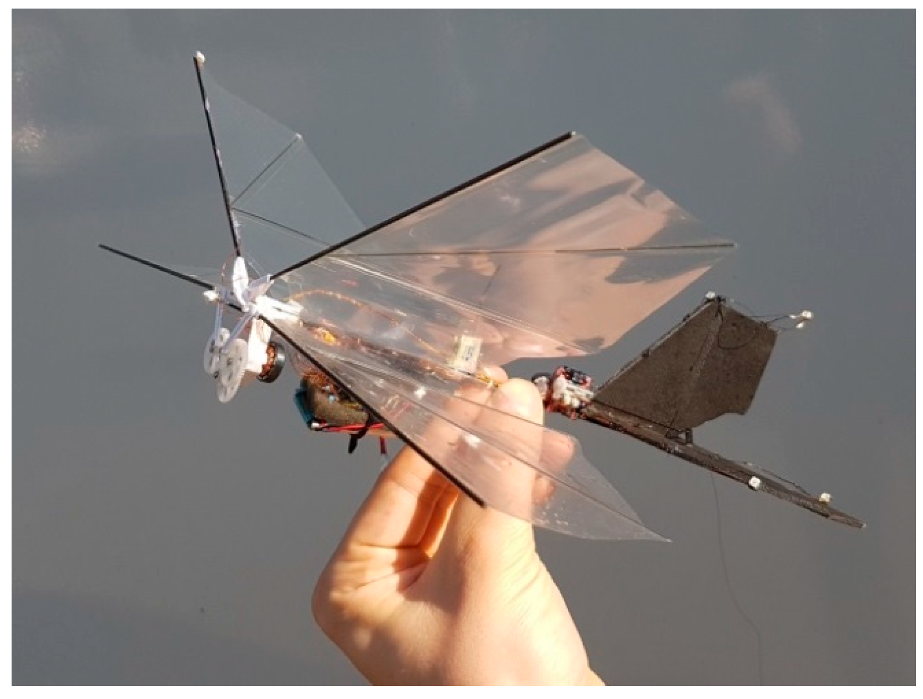
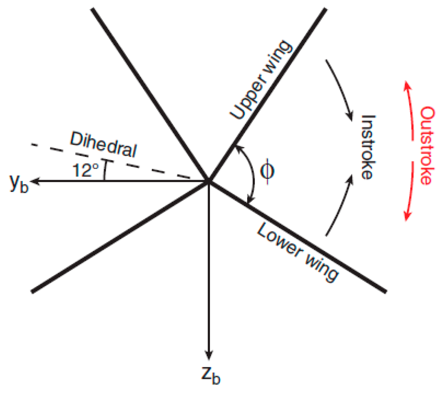
The DelFly MAV is a four-wing flapping MAV with wing pairs on either side of the vehicle that are set at a dihedral angle of 12° and actuated in counter-phase (see Figure 1 and Figure 2). The total wing span is 280 mm and the maximum stroke angle ϕ is 87°. The wings are constructed from 15 µm thick transparent Mylar foil, with carbon-fiber leading edge spars and wing stiffeners completing the wing structure. The leading edge spars are driven by a single motor through a gear-pushrod mechanism (see Figure 1) in a periodic, quasi-sinusoidal flapping motion, during which the wing surfaces undergo appreciable passive deformation [14,19]. Figure 2 defines the wing kinematics nomenclature based on the leading edge motion, with the outstroke being the phase in the flapping cycle where the wings move away from each other, and the instroke being the phase where they move towards each other. It is to be remarked that because of the wing flexibility, the wing surface motion displays an appreciable delay with respect to that of the driven leading edge. As a result, when the wings meet at the transition from the instroke to the outstroke, a so-called “clap-and-peel” occurs: as the wing leading edges move away from each other again, the wing surfaces only gradually come apart as the outstroke progresses. This is indeed clearly visible in the flow visualizations discussed in Section 3.1.
The mass of the DelFly model used in the experiments is approximately 25 g, and the total vehicle length is about 215 mm. The tail assembly has a span of 170 mm and is constructed from 2 mm thick Depron polystyrene sheet; it was painted black to reduce light reflections. The flight speed during the present tests is around 1 m/s, with the pitch angle and the flapping frequency being around 60° and 13.5 Hz, respectively. At these conditions, the distance over which the DelFly advances during a single wingbeat is approximately 7 cm.
2.2. The Flight Control System
The automatic control system used for this free-flight investigation is similar to the one used in [17], consisting of an optical motion tracking system and an onboard autopilot system. The tracking system is comprised of 24 cameras (OptiTrack Flex 13, Natural Point Inc., Corvallis, OR, USA), which were positioned on the ceiling of the flight arena for tracking the 7 infrared LED markers placed on the DelFly MAV (at the body, tail, wing and control surfaces). According to manufacturer specifications, the position tracking accuracy is better than 1 mm. The online position and orientation information obtained by the tracking system is fed via a wireless link (WiFi) to the onboard autopilot system (Lisa/S autopilot [20] with Paparazzi UAV software) to guide the DelFly in a prescribed trajectory through the measurement area. More technical details of the tracking system can be found in [17].
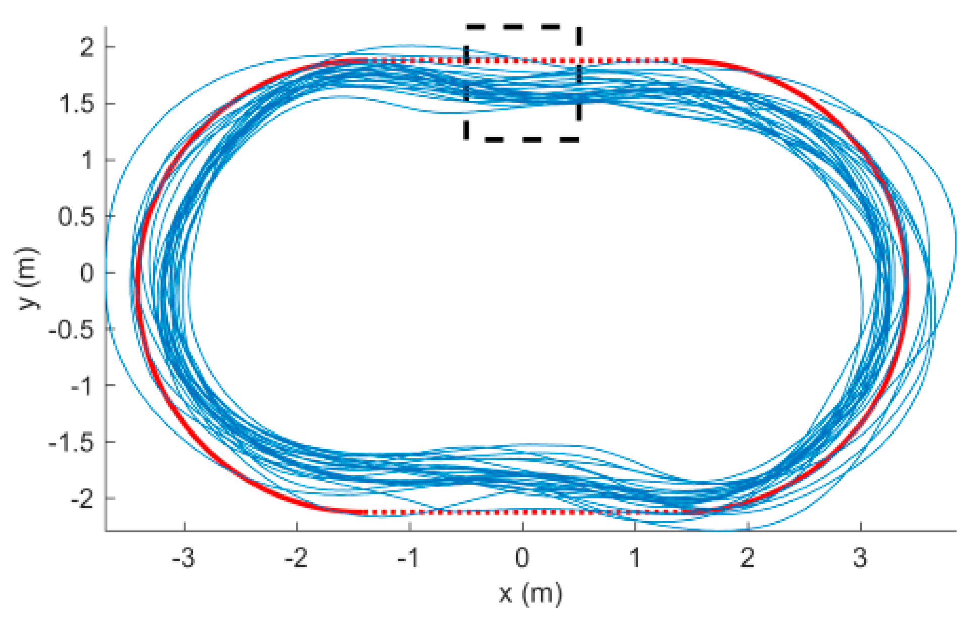
The DelFly vehicle was programmed to follow an oval trajectory, consisting of two half circles of 4 m in diameter, with two approximately 3 m long straight segments in between (see Figure 3). The guidance algorithm uses a “carrot” waypoint that the vehicle tries to reach. This waypoint is placed at a fixed distance in front of the vehicle on the desired flight path, and is advanced at every time step of the control loop to keep its distance from the vehicle constant. Despite the relatively sharp turns, this strategy results in repeatable trajectories that remain close to the desired path (Figure 3). The spread in the lateral direction was comparable to the wingspan of the vehicle, which enabled reliable repeated traversal of the 1 m wide test area. The accuracy of the height control was below 2.5 cm at optimum tracking conditions, which corresponds to about 10% of the wing span.
The area where the PIV measurements were performed was located approximately in the middle of one of the straight segments (see Figure 3), such that the vehicle would have time to recover to a steady flight state after the turn, and its trajectory would not interfere with the camera setup (see Section 2.3). Given the forward speed of 1 m/s, the vehicle crossed the test area approximately every 15 s. In view of the limited accuracy in the control of the lateral position of the vehicle (see above), which was further prone to disturbances such as drafts or lower tracking precision under the net covering the test area, an operator was monitoring the lateral position error from the desired flight path (both visually and via online telemetry), and could decide to redo the experiment during a next pass if the lateral error was too large. The PIV measurement was triggered by the operator prior to the moment when the vehicle would enter the test area (cf. Figure 4). This would also light up additional LED markers, detected by the motion tracking system, which was used to synchronize the motion tracking data with the PIV dataset. In this way, the vehicle position, orientation, and the wing stroke angle corresponding to each PIV frame could be determined.
2.3. The Particle Image Velocimetry (PIV) Procedure
The employed PIV technique uses nearly-neutrally-buoyant helium filled soap bubbles (HFSB; with approximate size of 300 μm) as extremely bright tracer particles that allow a large field of view to be measured [18], while at the same time mitigating the effect of the laser light reflections from the flapping wings. As the bubbles scatter significantly more light than micron-sized droplets (by approximately a factor of 10,000), the ratio of particle light intensity to the parasite wing reflection intensity is strongly increased. This enables flow field visualization to be achieved also relatively close to the wings, in contrast to previous PIV experiments, in which regular PIV seeding was used.
The experimental procedure is illustrated in Figure 5. The actual test area (approximate size of 1 m in width, length and open height) was filled with the helium-filled soap bubbles prior to the PIV measurements, and enclosed at the sides and the top with a fine-maze mosquito net to contain the bubbles so as to maintain a sufficient tracer concentration. A high-speed Nd:YAG laser (Mesa-PIV (Continuum, San Jose, CA, USA) at a wavelength of 532 nm and 18 mJ pulse energy) was employed to provide illumination from below in the form of a vertically projected laser light sheet. Two visualization configurations were used, differing in the orientation of the light sheet with respect to the MAV flight path. Firstly, planar (2-component) PIV measurements were performed in a streamwise (i.e., chordwise) aligned plane. For this purpose, a single high-speed camera (Photron Fastcam SA-1.1 (Photron, San Diego, CA, USA), 1 Megapixel) was employed to record images of the HFSB tracers. Subsequently, two high-speed cameras in a stereoscopic configuration were used to obtain all three velocity components in a spanwise-aligned measurement plane capturing the flow field during the passage of the DelFly model. The two imaging configurations are illustrated in the schematics in Figure 5. In both cases, the field of view is approximately 350 × 350 mm2 and the image recording rate 2 kHz, corresponding to approximately 140–150 images per flapping cycle. At a maximum observed flow velocity of about 5 m/s, the corresponding particle displacement between subsequent images is 8 pixels. Time-series of single-frame images were interrogated with a final window size of 48 × 48 pixels with an overlap factor of 75%, yielding a vector resolution of 3.8 mm at a flow velocity accuracy of about 0.1 m/s.
3. Results and Discussion
3.1. Streamwise Planar Flow Visualizations
In the first measurement configuration, the light sheet is oriented parallel to the flight direction (see also Figure 4), and visualizes a streamwise plane that intersects the MAV wings at a specific spanwise position, which is determined by the lateral displacement of the flight path with respect to the light sheet. The latter proved difficult to control accurately, providing only limited control over the spanwise location of the imaged measurement plane. Two useful datasets were obtained, corresponding to intersections at 45 ± 4% (S1) and 63 ± 3% (S2) of the half-span of the wings, respectively. The flight conditions were similar for both cases (flight speed 1.0 ± 0.1 m/s, pitch angle 61–62° and flapping frequency 13.4 ± 0.1 Hz). At these conditions, a full crossing of the field of view is performed in 0.35 s, which corresponds to approximately 5 flapping cycles, comprising a dataset of about 700 images.
3.1.1. Results for the 45% Half-Span Visualization (S1)
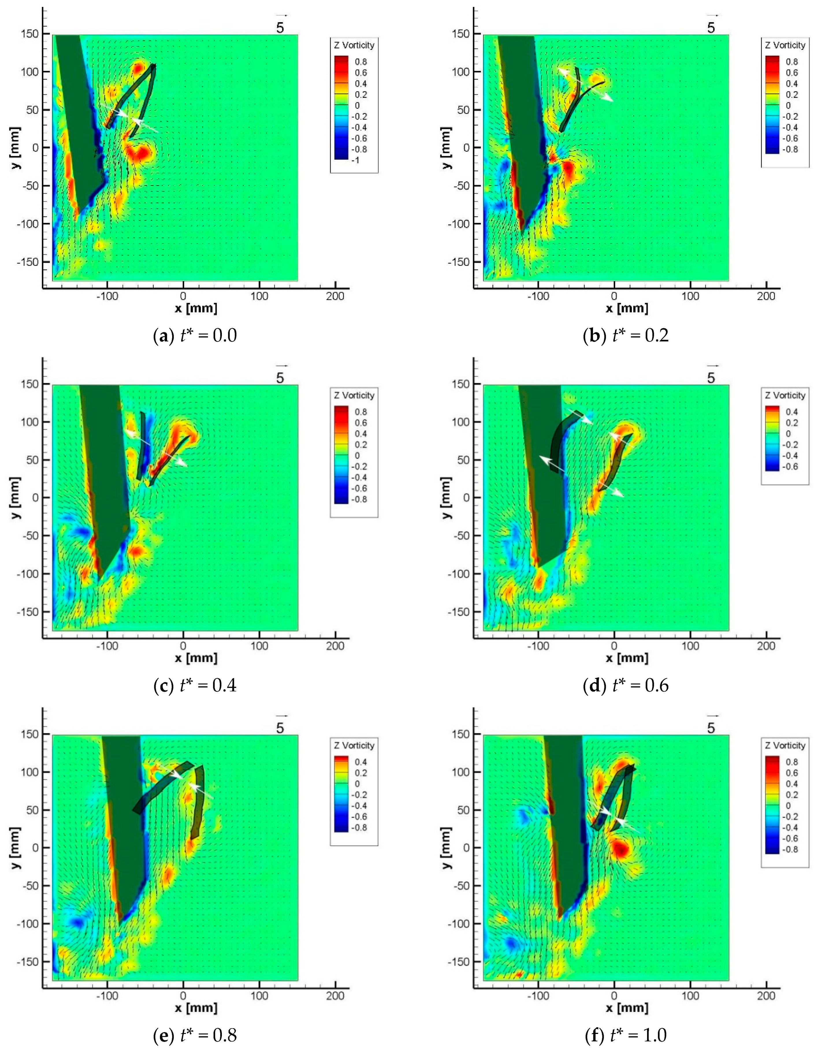
Flow structures in a chordwise-oriented plane at approximately 45% of the semi-span (dataset S1) are shown in Figure 6, for subsequent phases covering one complete flapping cycle. Non-dimensional time is defined as t* = t/T (T = 1/f being the flapping period) with t* = 0 corresponding to the moment of the stroke direction reversal that marks the end of the instroke and the beginning of the outstroke. Note that the (x,y) coordinates used in the image frame correspond to the (x,z) directions of the flight path orientation, as indicated in Figure 4.
The position and cross-sectional shape of the two wings are clearly visible, and reflect the advancement of the MAV in the flight direction (i.e., towards the right) as time progresses. In the shaded region, the illumination is obstructed by the horizontal tail surface, which prevents meaningful measurements to be performed in that area. The white arrows have been inserted to indicate the relative motion of the wings with respect to each other, and it can be seen that shortly after stroke reversal, the wing flexibility results in an apparent rotation of the wings, with the wing LE and TE moving in opposite directions (see t* = 0.6, a similar behavior occurs near t* = 0.1). Also, in the early phase of the outstroke (see t* = 0.2) the visualization gives clear evidence of the “clap-and-peel” effect [14,19], where the rear part of the wings remain connected during much of the initial phase of the outstroke. As soon as the peel ends and the wing gap is opened, a strong downward flow between the wings is established, as can be seen at t* = 0.4, and which is maintained until the end of the instroke phase, see t* = 0.8.
The visualizations give furthermore clear evidence that the flow conditions, under the combined effect of forward velocity, high pitch angle, and wing flapping motion, result in asymmetric flow patterns being generated around the wings. For example, at t* = 0.4, which is towards the end of the outstroke, the lower (=right) wing has a much more coherent leading-edge vortex (LEV) than the upper wing. This can be attributed to the smaller effective velocity of the upper (=left) wing due to the forward motion of the DelFly, which also decreases the effective angle of attack and mitigates the flow separation (compare the results of [16]). It may be hypothesized that most of the lift (vertical force, in y direction) is hence generated by the lower wing in this phase, whereas the upper wing mostly accounts for the thrust (horizontal force, in the x direction). It can be further observed that towards the end of the instroke (t* = 1.0), the lower wing has released a large trailing-edge starting vortex (TEV) into the wake. Most likely a TEV of opposite vorticity is released by the upper wing, but its signature is blocked by the laser shadow region of the tail. Simultaneously during the instroke, an LEV is built up at the upper wing; both features can also be observed at t* = 0.0, confirming the periodicity of the flow. Closer observation suggests that these vortical structures are indeed already formed at t* = 0.8, but are less prominent, and therefore more difficult to detect in the PIV results; visual inspection of the particle image recordings supports this assumption (see Supplementary Material Video S1).
3.1.2. Results for the 63% Half-Span Visualization (S2)
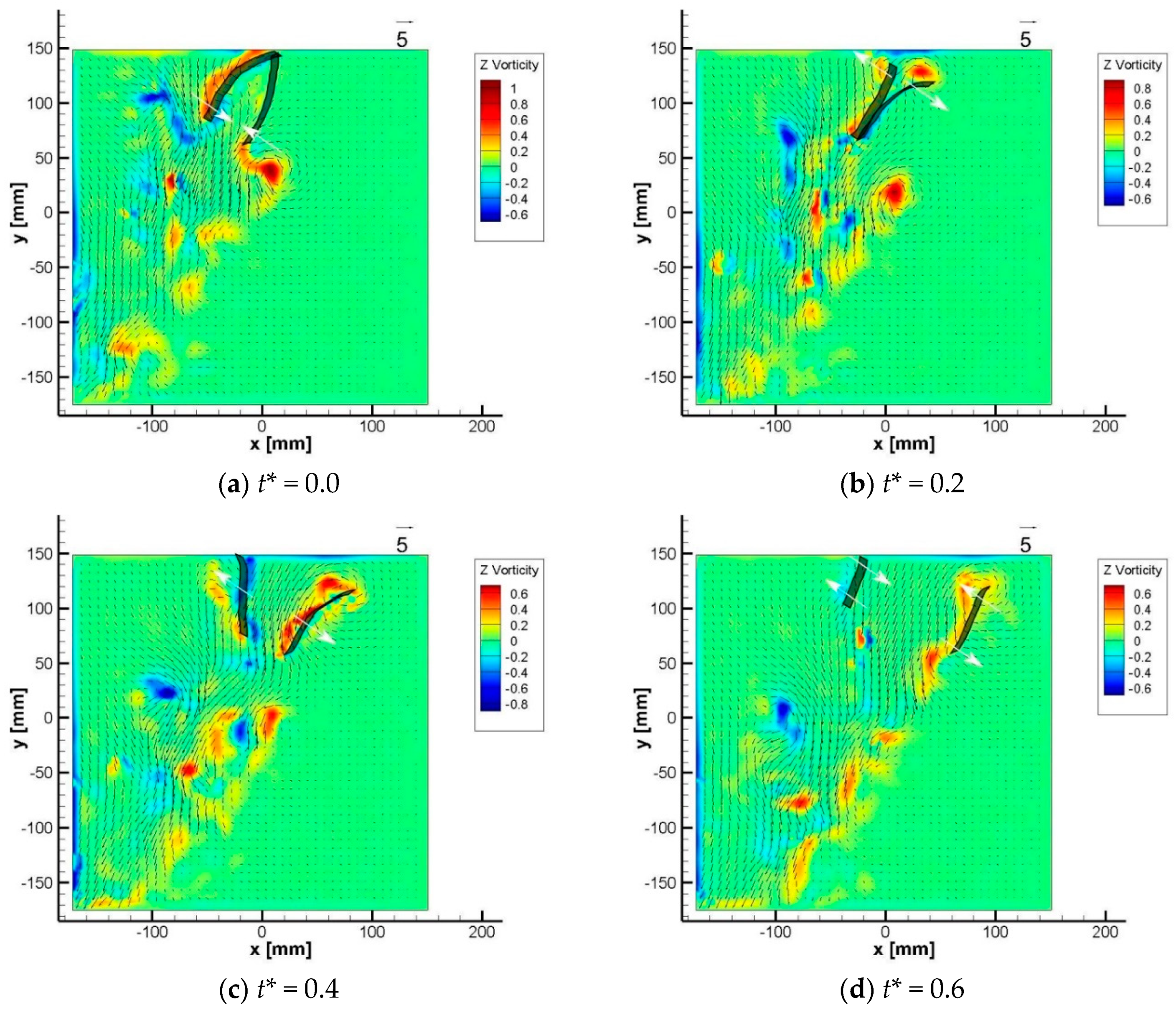
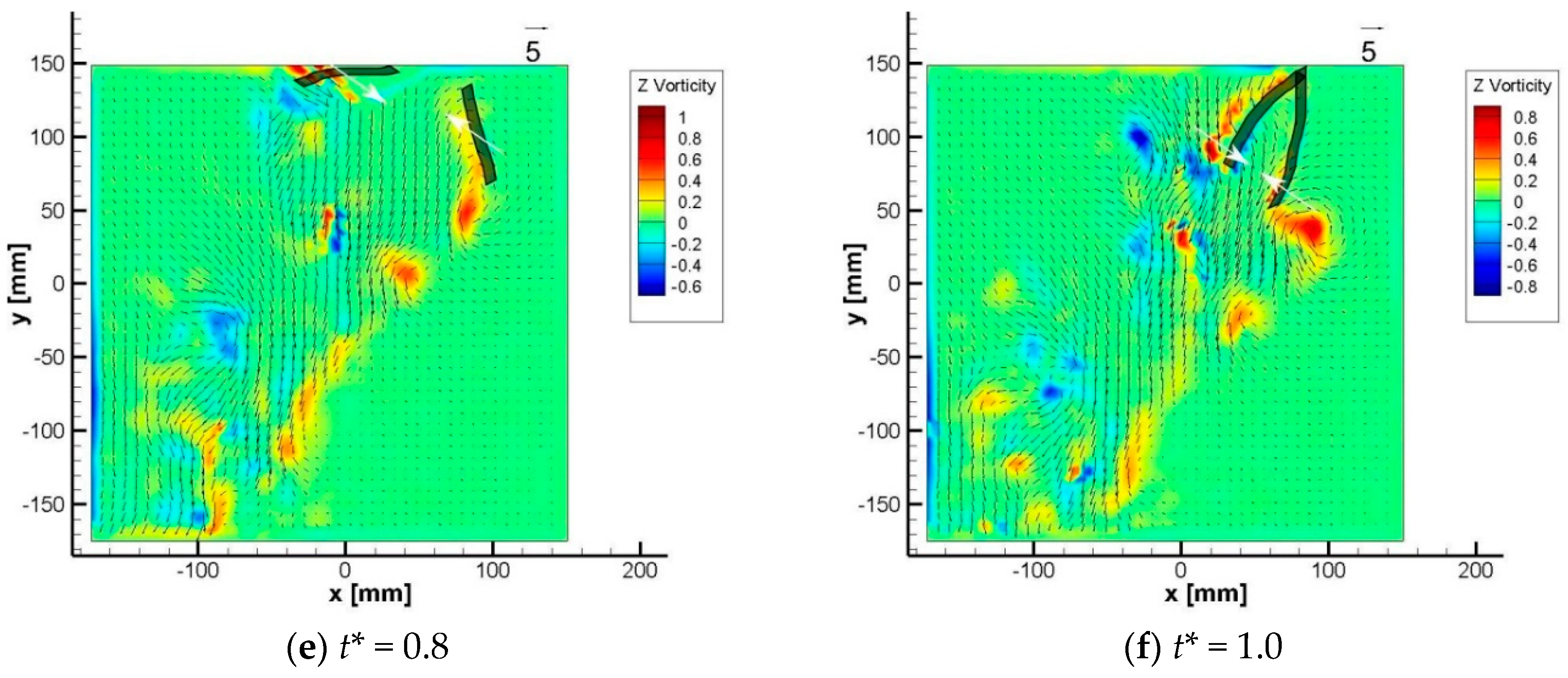
Flow structures in the chordwise-oriented plane at approximately 63% of the semi-span of the wing (dataset S2) are shown in Figure 7, for subsequent phases covering one complete flapping cycle. Note that the S2 position (at 63% semi-wing span) is located more outboard than the S1 position (at 45% semi-wing span), and corresponds approximately to the tip of the horizontal tail surface (which is at 61% of the semi-wing span). This explains why there is no significant shadow effect of the tail surface shielding part of the measurement as in the case of S1 (Figure 6), and it provides an unobstructed view of the flow field at this cross-section. However, during this passage, the DelFly flight path was approximately 50 mm higher with respect to the observation field, such that the upper regions of the wings are close to the edge of the field of view. In consequence, this imposes some restrictions on the information that is obtained about the flow structures generated around the wing leading edges, yet a clearer view of the entire wake is provided. The wing motion and deformation patterns are very similar to those of the more inboard visualization (S1). The wings move further apart in the outstroke (compare Figure 7d to Figure 6d), which is a logical consequence of the flapping-wing configuration (see Figure 1 and Figure 2). This notwithstanding, comparing Figure 7b to Figure 6b allows us to conclude that the peeling of the wings has advanced to a further stage at the more outboard position, which has also been observed in static high-speed visualizations [19]. Regarding the generated flow structures, these are consistent with the observations for the S1 plane. It is confirmed that at the instroke, also the upper wing indeed generates a TEV, albeit one that is weaker in circulation strength than that of the lower wing. This may be surprising, as the relative velocity of the upper wing is larger, with the body velocity adding to the relative wing motion; a possible explanation can be that at this high pitch angle, the upper wing is shielded by the presence of the lower wing.
3.2. Analysis of the Flow-Induced Effect of the Flapping Wings
In an effort to quantify the propulsive effect of the flapping wings, the relative induced acceleration of the flow is assessed on the basis of a momentum analysis by comparing the upstream and downstream conditions near the wings (constrained to the two dimensional flow data provided by the 2C PIV method). For this purpose, the flow velocity results from the S1 and S2 datasets are monitored at two points in the flow field in relative position with respect to the MAV, denoted by the “inlet” and the “outlet”, thus tentatively comparing the gap between the wings to a propulsive channel. These points are located in the dihedral plane between the wings, slightly above the leading edge and below the trailing edge, respectively, and advanced with the motion of the MAV. Inaccuracies in the procedure of defining these points are likely to contribute to fluctuations in the velocity results.
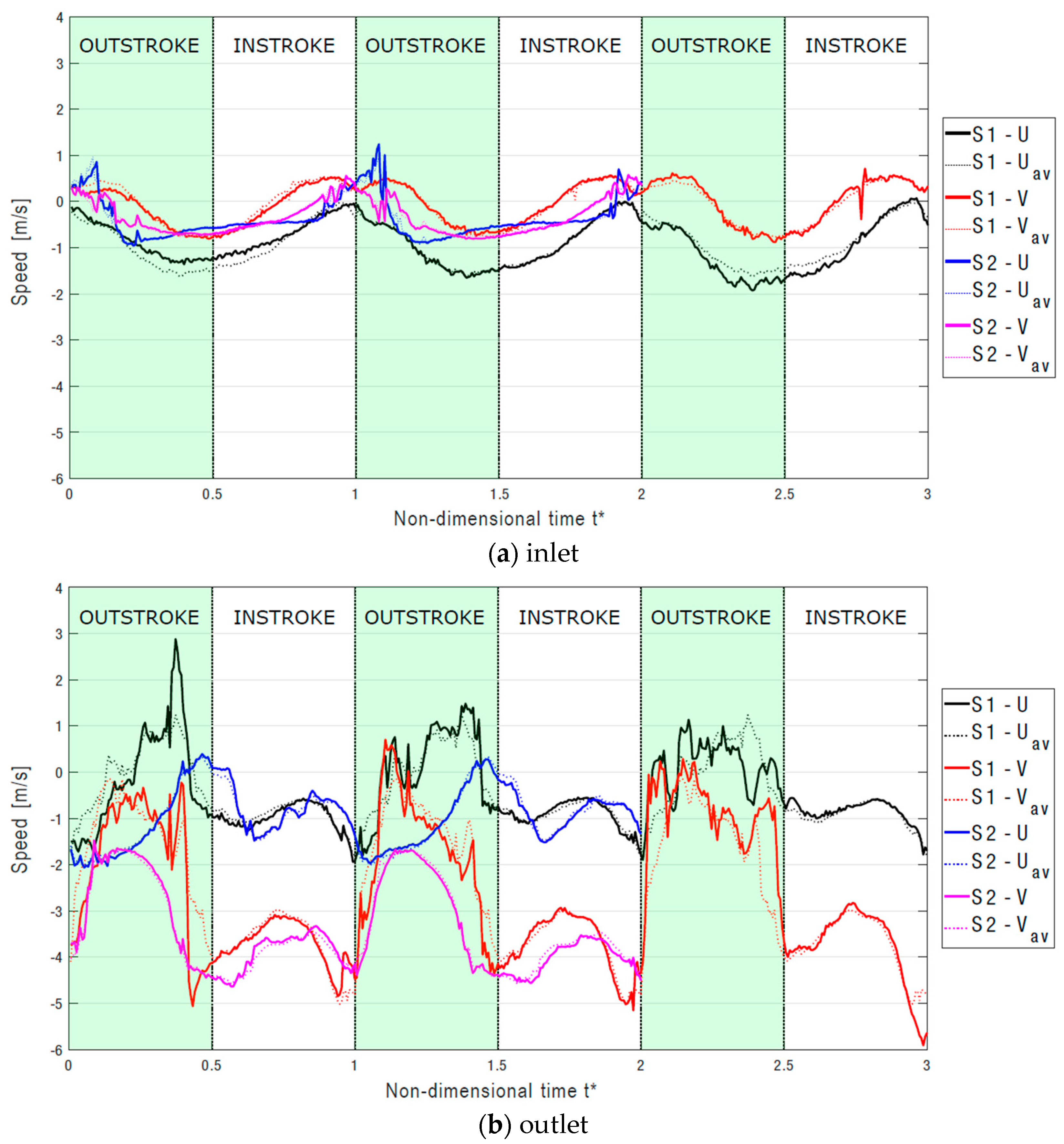
Figure 8 shows the results for the flow velocity components at these two monitoring positions for the available full flapping cycles for each experiment (three cycles for S1 and two cycles for S2), with the datasets synchronized at t* = 0 for the onset of the outstroke. The positive directions for U and V are to the right and upward, respectively, in accordance to Figure 6 and Figure 7. The solid lines indicate the actual variations over the individual cycles, while the dashed lines represent phase-averaged results, which allows us to verify the periodicity of the results. The higher level of fluctuations for S1 are attributed to the circumstance that at this inboard location the disturbing effect of the wing reflections is larger than for the outboard location S2 due to the closer proximity of the wings and the wing deformations.
It can be observed in Figure 8a that for the inlet position, the velocity variation is relatively small and displays in general a very periodic trend. Velocities are seen to decrease (i.e., become more negative) during the outstroke, and to increase during the instroke, which is consistent with the induced flow generated near the wing leading edges in these phases of the flapping cycle. For the outlet position (Figure 8b), much stronger variations occur, with a distinctly different pattern for the instroke and outstroke phases, especially regarding the vertical velocity component. During much of the outstroke, the vertical velocity remains relatively small in magnitude, and more so for the inboard location (S1) than for the outboard one (S2). This reflects the inhibition of the downward flow by the closure of the wing gap during the “peel phase” (compare Figure 6b). Once this gap is fully opened (which occurs around t* = 0.4), and also during the subsequent instroke, the vertical velocity reaches large negative values, indicating a strong downward induced flow. The horizontal velocity component shows less variation, which is likely due to the high pitch angle of the DelFly, apart from occasional peaks in the force signal that may be due to measurement uncertainty and the occurrence of vortices near the wing leading edges.
Assessing the cycle-averaged velocity values, we find (see Table 1) for the vertical velocity component V a negative change between outlet and inlet velocities (−2.59 m/s for S1 and −3.07 m/s for S2), which is consistent with an upward reaction force, i.e., lift. For the horizontal velocity component U, we find a positive change of +0.47 m/s for S1 (i.e., a net drag at the more inboard location) and a negative change of −0.61 m/s for S2 (i.e., a net thrust at the more outboard location).
3.2.1. Estimation of Flow Conditions Perceived by the Tail
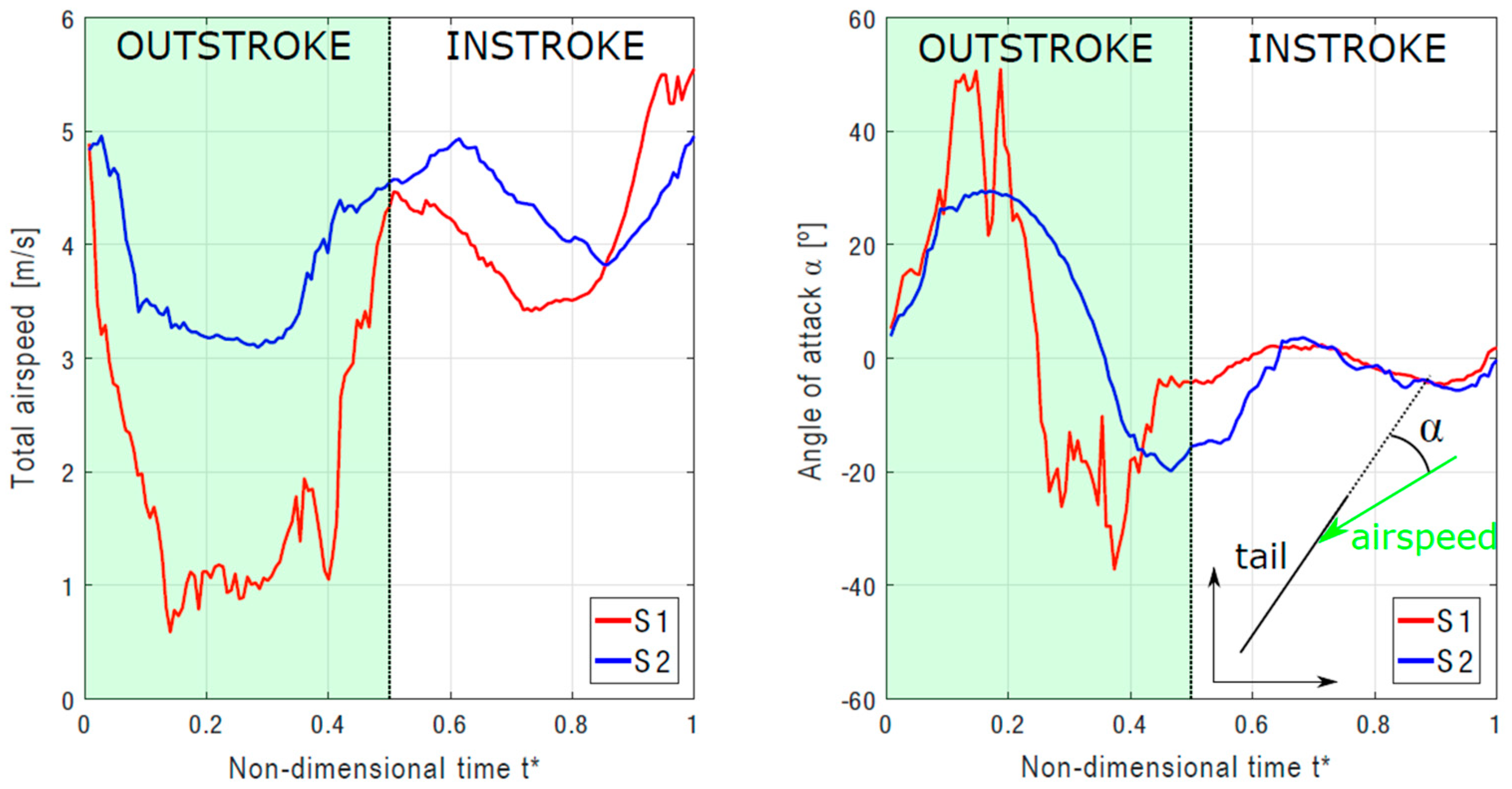
A second aspect of relevance for the performance of a flapping-wing MAV of the current configuration, being equipped with a conventional tail assembly, is how the flow conditions near the tail are affected by the strong periodic variations of the wake flow of the flapping wings. For this, an estimate is made of the flow conditions perceived by the tail, by taking into account the flow induced by the wings in combination with the forward flight speed. Next, the flow conditions are expressed in terms of the absolute velocity magnitude and the effective angle of attack relative to the plane of the horizontal tail surface. Assuming a horizontal flight of the MAV, the absolute flow speed and angle of attack at the tail are calculated as:
where and are the flow velocity components at the outlet position (as in Figure 8b), while and are the flight speed and pitch angle of the MAV. The results for and are given in Figure 9. Note that the S2 position (at 63% semi-wing span) corresponds approximately to the tip of the horizontal tail surface (which is at 61% of the semi-wing span), whereas the S1 position (at 45% semi-wing span) corresponds to approximately 75% of the tail semi-span. It is observed that over most of the flapping cycle, the absolute airspeed is quite high (between 3 and 5 m/s) compared to the flight speed (~1 m/s). For reference, this may be compared to the mean wing tip speed (~5 m/s) or the average induced speed estimated from actuator disk theory (which is ca. 2.7 m/s). From the results shown in Figure 9, it is observed that during the outstroke, the angle of attack is first positive and then negative; however, the airspeed remains relatively low during the outstroke. During the instroke, on the other hand, the airspeed is high, yet the angle of attack remains near zero.
Although a further exposure of the design implications of these results is beyond the scope of the present paper, information on the flow conditions near the tail is expected to be supportive to the modeling of wing-wake/tail interactions [21], and to further interpret “black-box” data on tail surface sizing and tail effectiveness [22].
3.3. Spanwise Planar Flow Visualizations
In the second visualization configuration, the illumination plane is normal to the flight direction, and visualizes the flow development as the MAV passes through the light sheet, which is captured by the stereoscopic PIV configuration (see Figure 5b). The practical aspects of this visualization approach are simpler, in the sense that they are less sensitive to the precise lateral and vertical positioning of the flight path. However, the interpretation of the visualizations proved to be more complex, because the measurement plane position is not fixed with respect to the MAV. As a result, the flow structures that are observed in the measurement plane depend on both the position of the MAV relative to the light sheet, as well as on the flapping phase of the wings, and can be further complicated when the MAV crosses the plane with a yaw or sideslip angle. Removal of this ambiguity in the flow visualization would best be served by a true volumetric method, see e.g., [23,24], but such is as yet not really feasible for the considered conditions. Nevertheless, the obtained results were found to be informative regarding the generation of streamwise vortical structures during the flapping cycle.
Results are presented for one of the recordings where the MAV enters the field-of-view approximately at beginning of the outstroke (t* = 0), while at the end of the instroke (t* = 1) the MAV has crossed the light sheet, such that only the tail is illuminated. This has as a clear implication that the recordings at t* = 0 and t* = 1 are likely not to give identical flow patterns, in contrast to the streamwise flow visualization strategy (compare Figure 6a to Figure 6f, for example).
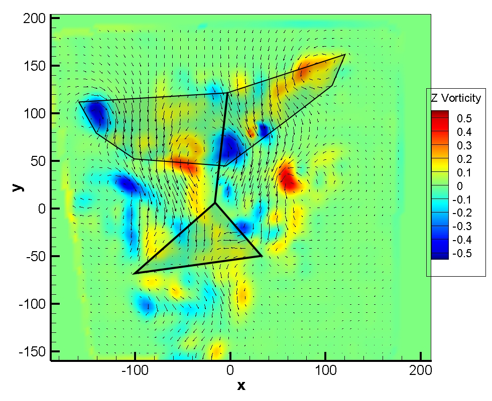
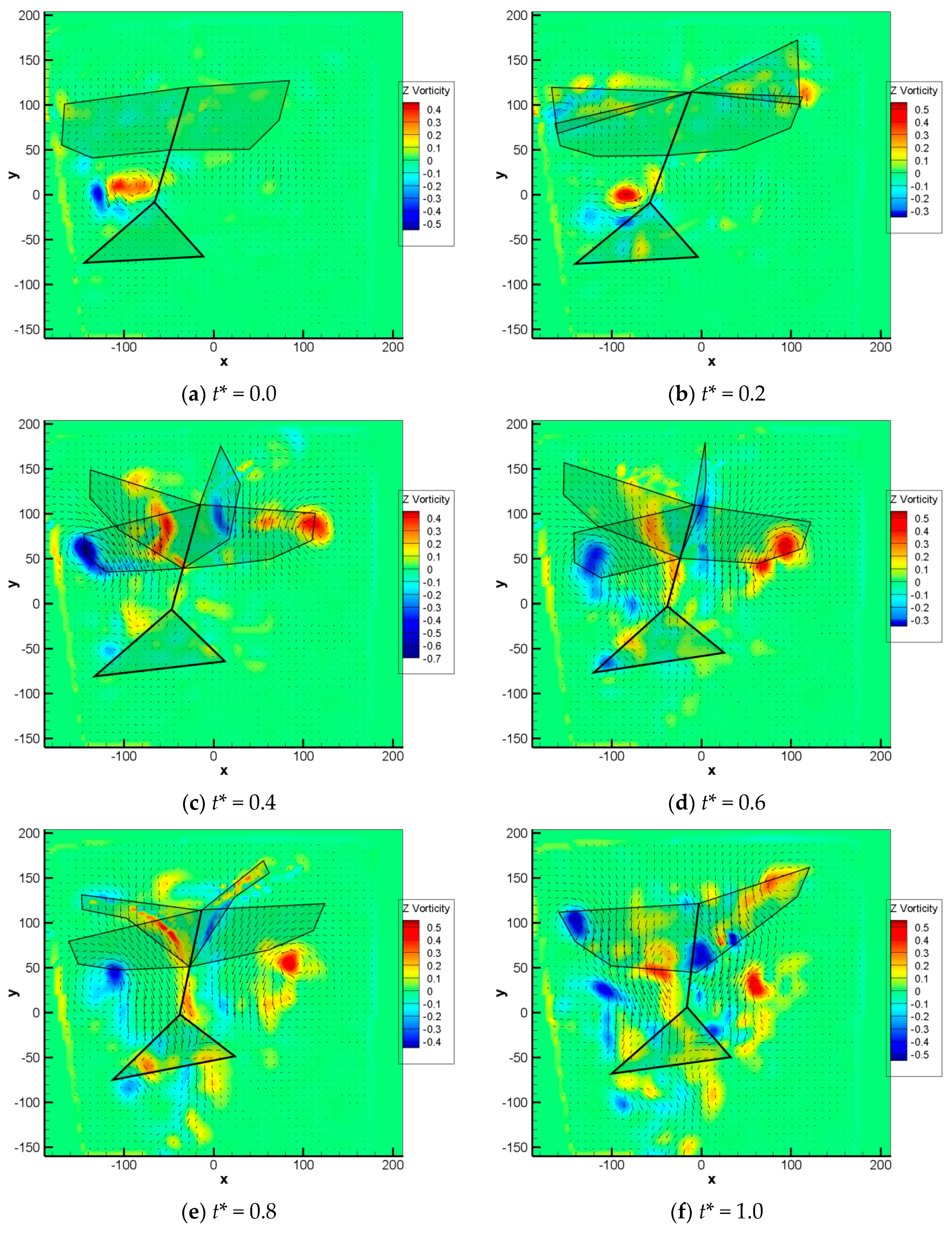
Contours of out-of-plane vorticity covering the flapping cycle from t* = 0 to t* = 1 are shown in Figure 10. It should be noted that the DelFly model outline is meant here to assist in the interpretation of the flow visualizations, but is indicative only. Note furthermore that the (x,y) coordinates in the image frame correspond to the (y,z) directions of the flight path orientation, as indicated in Figure 4. The vorticity color coding allows visualization of prominent rotational flow structures (longitudinal vortices), bearing in mind that that the streaky vorticity structures that occur halfway the wings in for example Figure 10c–e are measurement artefacts caused by laser light reflections on the deformed upper wings.
At t* = 0 (Figure 10a), two counter-rotating vortical structures can be seen which would appear to be created shortly before this moment, and which decay in the subsequent phases. Their origin is not directly obvious, also in view of the fact that similar structures do not always occur in the same form in other recordings, which leads to the assumption that they are in some way connected to the asymmetric flight path in this case. During the outstroke (see Figure 10b,c), prominent counter-rotating vortices are generated at the tips of the lower wings, which remain visible in the measurement plane during the whole remainder of the visualization cycle while the DelFly proceeds forward. This is directly indicative that during the outstroke, the lower wings are actively generating lift (which supports the statement made in Section 3.1), while the upper wings are relatively inactive in this respect. It is only towards the end of the instroke (Figure 10f) that tip vortices generated by the upper wings become clearly visible. The orientation of the vortices is the same as that previously observed for the lower wings during the outstroke, which confirms that during the instroke, only the upper wings are generating lift. At the same time, counter-rotating vortices are visible near the wing roots. The most likely explanation for why similar root vortices are not generated during the outstroke is that due to the clap-and-peel, the wings separate only gradually, which suppresses vortex formation especially near the root region. Throughout most of the flapping cycle, small scale vortical structures can be seen in the region near the tail, however, it is not clear if these are indeed related to vibrations of the tail or substructures within the wing wake.
4. Conclusions
Flow visualizations have been performed on a flapping-wing Micro Air Vehicle (MAV) in free flight, using an innovative large-scale particle image velocimetry (PIV) approach. The PIV methodology involves the use of helium filled soap bubbles (HFSB). The specific objective of the investigation is to provide a quantitative flow characterization of the flapping-wing MAV under unconstrained conditions, which are fully representative of actual flight. The followed large-scale PIV strategy is especially instrumental in this, as it expands the flow visualization capabilities significantly. To summarize the major benefits of this PIV approach: (1) the application of highly reflective HFSB tracers allows a relatively large scale domain to be illuminated with a high-repetition laser (of even moderate power), such that time-resolved information can be obtained, which removes the need to rely on phase-averaging; (2) the high brightness of the tracer particles mitigates relative wing-reflection effects, such that flow visualization can be achieved even relatively close to the wings.
Measurements on the MAV were performed in two configurations that differ in the orientation of the light sheet with respect to the flight direction. In the first configuration, the light sheet is parallel to the flight direction, and visualizes a streamwise plane that intersects the MAV wings at a specific spanwise position. In the second configuration, the illumination plane is normal to the flight direction, and visualizes the flow as the MAV passes through the light sheet.
The results permit the identification of the different aerodynamic behavior of upper and lower wings in actual forward flight conditions, as well as the generation of streamwise vortices by the wings and possibly the tail as well. From this we can conclude that the lower wings are the most aerodynamically active in generating lift in the outstroke phase, and the upper wings during the instroke (see Section 3.3). Conversely, as regards the generation of thrust, the role of the wings is opposite to that of the lift generation: the upper wings are the most aerodynamically active in the outstroke phase, and the lower wings during the instroke (see Section 3.1). The measurement results were further used to estimate the flow conditions near the MAV tail (Section 3.2.1), which is of relevance for the flight performance in terms of control and stability. Although a full exposure of the design implications of these results is beyond the scope of the present paper, information on the flow conditions near the tail is expected to be supportive to the modeling of wake/tail interactions and the interpretation of “black-box” flight control data [21,22].
Challenges encountered in these planar visualizations measurements were associated with the control of the spanwise location of the intersection for the streamwise visualization, as a result of the limited flight control authority in the test area itself. For the spanwise visualization, the simultaneous dependence on both the flapping phase of the wings and the MAV position with respect to the light sheet affects an unambiguous interpretation of the flow structures. These issues could in principle be resolved with a volumetric visualization approach at a sufficiently large scale, but this is currently not yet achievable with off-the-shelf PIV equipment. Although a few large-scale volumetric studies have been reported [23,24], the general applicability of such approaches is currently limited by the required high laser power for the volume illumination, the low-to-moderate repetition rate of these PIV lasers, and, in consequence of the latter, the necessity for phase-averaging data strategies.
Supplementary Materials
The following are available online at https://www.mdpi.com/2226-4310/5/4/99/s1, Video S1 (Movie_1.avi): Particle image recording for streamwise visualization (one complete flapping cycle).
Author Contributions
Conceptualization and Supervision: M.P. and B.v.O.; Experiment Design, Methodology and Investigation: M.P., A.d.E.H. and M.K.; Data Analysis: A.d.E.H. and M.P.; Data Reporting, Validation and Visualization: A.d.E.H.; Text Original Draft Preparation: A.d.E.H., B.v.O. and M.P.; Text Contributions, Corrections and Review: all authors; Manuscript Final Editing: B.v.O.
Acknowledgments
A.d.E.H. was supported by the ERASMUS+ program.
Conflicts of Interest
The authors declare no conflict of interest.
Abbreviations
The following abbreviations are used in this manuscript:
| FOV | Field of View |
| HFSB | Helium Filled Soap Bubbles |
| LEV | Leading Edge Vortex |
| MAV | Micro Air Vehicle |
| PIV | Particle Image Velocimetry |
| TEV | Trailing Edge Vortex |
References
- Wood, R.J. The first takeoff of a biologically inspired at-scale robotic insect. IEEE Trans. Robot. 2008, 24, 341–347. [Google Scholar] [CrossRef]
- Keennon, M.; Klingebiel, K.; Won, H.; Andriukov, A. Development of the nano hummingbird: A tailless flapping wing micro air vehicle. In Proceedings of the 50th AIAA Aerospace Sciences Meeting, Nashville, TN, USA, 9–12 January 2012. Paper AIAA 2012-0588. [Google Scholar] [CrossRef]
- de Croon, G.C.H.E.; Percin, M.; Remes, B.D.W.; Ruijsink, R.; de Wagter, C. The DelFly: Design, Aerodynamics, and Artificial Intelligence of a Flapping Wing Robot, 1st ed.; Springer: Heidelberg/Berlin, Germany, 2016; ISBN 978-94-017-9208-0. [Google Scholar]
- Ramezani, A.; Chung, S.-J.; Hutchinson, S. A biomimetic robotic platform to study flight specializations of bats. Sci. Robot. 2017, 2, eaal2505. [Google Scholar] [CrossRef]
- Sane, S.P. The aerodynamics of insect flight. J. Exp. Biol. 2003, 206, 4191–4208. [Google Scholar] [CrossRef] [PubMed] [Green Version]
- Nguyen, Q.V.; Truong, Q.T.; Park, H.C.; Goo, N.S.; Byun, D. Measurement of force produced by an insect-mimicking flapping-wing system. J. Bionic Eng. 2010, 7, 94–102. [Google Scholar] [CrossRef]
- Lin, C.-S.; Hwu, C.; Young, W.-B. The thrust and lift of an ornithopter’s membrane wings with simple flapping motion. Aerosp. Sci. Technol. 2006, 10, 111–119. [Google Scholar] [CrossRef]
- Lee, J.-S.; Han, J.-H. Experimental study on the flight dynamics of a bioinspired ornithopter: Free flight testing and wind-tunnel testing. Smart Mater. Struct. 2012, 21, 094023. [Google Scholar] [CrossRef]
- Percin, M.; van Oudheusden, B.; Eisma, H.; Remes, B. Three-dimensional vortex wake structure of a flapping-wing micro aerial vehicle in forward-flight configuration. Exp. Fluids 2014, 55, 1806. [Google Scholar] [CrossRef]
- Caetano, J.V.; Percin, M.; van Oudheusden, B.W.; Remes, B.; De Wagter, C.; de Croon, G.C.H.E.; de Visser, C.C. Error analysis and assessment of unsteady forces acting on a flapping wing micro air vehicle: Free flight versus wind-tunnel experimental methods. Bioinspir. Biomim. 2015, 10, 056004. [Google Scholar] [CrossRef] [PubMed]
- Johansson, L.C.; Hedenström, A. The vortex wake of blackcaps (Sylvia atricapilla L.) measured using high-speed digital particle image velocimetry (DPIV). J. Exp. Boil. 2009, 212, 3365–3376. [Google Scholar] [CrossRef] [PubMed]
- Hubel, T.Y.; Riskin, D.K.; Swartz, S.M.; Breuer, K.S. Wake structure and wing kinematics: The flight of the lesser dog-faced fruit bat, Cynopterus brachyotis. J. Exp. Boil. 2010, 213, 3427–3440. [Google Scholar] [CrossRef] [PubMed]
- Muijres, F.T.; Johansson, L.C.; Barfield, R.; Wolf, M.; Spedding, G.R.; Hedenström, A. Leading-edge vortex improves lift in slow-flying bats. Science 2008, 319, 1250–1253. [Google Scholar] [CrossRef] [PubMed]
- De Clercq, K.M.E.; de Kat, R.; Remes, B.; van Oudheusden, B.W.; Bijl, H. Aerodynamic experiments on DelFly II: Unsteady lift enhancement. Int. J. Micro Air Veh. 2009, 1, 255–262. [Google Scholar] [CrossRef]
- Percin, M.; van Oudheusden, B.W.; Remes, B. Flow structures around a flapping-wing micro air vehicle performing a clap-and-peel motion. AIAA J. 2017, 55, 1251–1264. [Google Scholar] [CrossRef]
- Deng, S.; van Oudheusden, B.W. Wake structure visualization of a flapping-wing micro-air-vehicle in forward flight. Aerosp. Sci. Technol. 2016, 50, 204–211. [Google Scholar] [CrossRef]
- Karasek, M.; Percin, M.; Cunis, T.; van Oudheusden, B.W.; De Wagter, C.; Remes, B.D.W.; de Croon, G.C.H.E. First free-flight flow visualisation of a flapping-wing robot. arXiv 2016, arXiv:1612.07645. [Google Scholar]
- Scarano, F.; Ghaemi, S.; Caridi, G.C.A.; Bosbach, J.; Dierksheide, U.; Sciacchitano, A. On the use of helium-filled soap bubbles for large-scale tomographic PIV in wind tunnel experiments. Exp. Fluids 2015, 56, 42. [Google Scholar] [CrossRef]
- Percin, M.; van Oudheusden, B.W.; de Croon, G.C.H.E.; Remes, B. Force generation and wing deformation characteristics of a flapping-wing micro air vehicle ‘DelFly II’ in hovering flight. Bioinspir. Biomim. 2016, 11, 036014. [Google Scholar] [CrossRef] [PubMed]
- Remes, B.D.W.; Esden-Tempski, P.; van Tienen, F.; Smeur, E.; De Wagter, C.; de Croon, G.C.H.E. Lisa-S 2.8g autopilot for GPS-based flight of MAVs. In Proceedings of the IMAV 2014: International Micro Air Vehicle Conference and Competition 2014, Delft, The Netherlands, 12 August 2014. [Google Scholar] [CrossRef]
- Armanini, S.F.; de Visser, C.C.; de Croon, G.; Caetano, J.V. Modelling wing wake and tail-wake interaction of a clap-and-peel flapping-wing MAV. In Proceedings of the AIAA Modeling and Simulation Technologies Conference, Denver, CO, USA, 5–9 June 2017. Paper AIAA 2017-0581. [Google Scholar] [CrossRef]
- Rijks, F.G.J.; Karásek, M.; Armanini, S.F.; de Visser, C.C. Studying the effect of the tail on the dynamics of a flapping-wing MAV using free-flight data. In Proceedings of the AIAA Atmospheric Flight Mechanics Conference, Kissimmee, FL, USA, 8–12 January 2018. Paper AIAA 2018-0524. [Google Scholar] [CrossRef]
- Henningsson, P.; Michaelis, D.; Nakata, T.; Schanz, D.; Geisler, R.; Schröder, A.; Bomphrey, R.J. The complex aerodynamic footprint of desert locusts revealed by large-volume tomographic particle image velocimetry. J. R. Soc. Interface 2015, 12, 0119. [Google Scholar] [CrossRef] [PubMed]
- Martínez Gallar, B.; van Oudheusden, B.W.; Sciacchitano, A.; Karasek, M. Large-scale flow visualization of a flapping-wing micro air vehicle. In Proceedings of the 18th International Symposium on Flow Visualization, Zurich, Switzerland, 26–29 June 2018. [Google Scholar] [CrossRef]
Figure 1.
The DelFly MAV used in the experiments.

Figure 2.
Wing motion definitions.

Figure 3.
The nominal (red) and realized (blue) flight trajectories, with the approximate test area location indicated in black.
Figure 3.
The nominal (red) and realized (blue) flight trajectories, with the approximate test area location indicated in black.

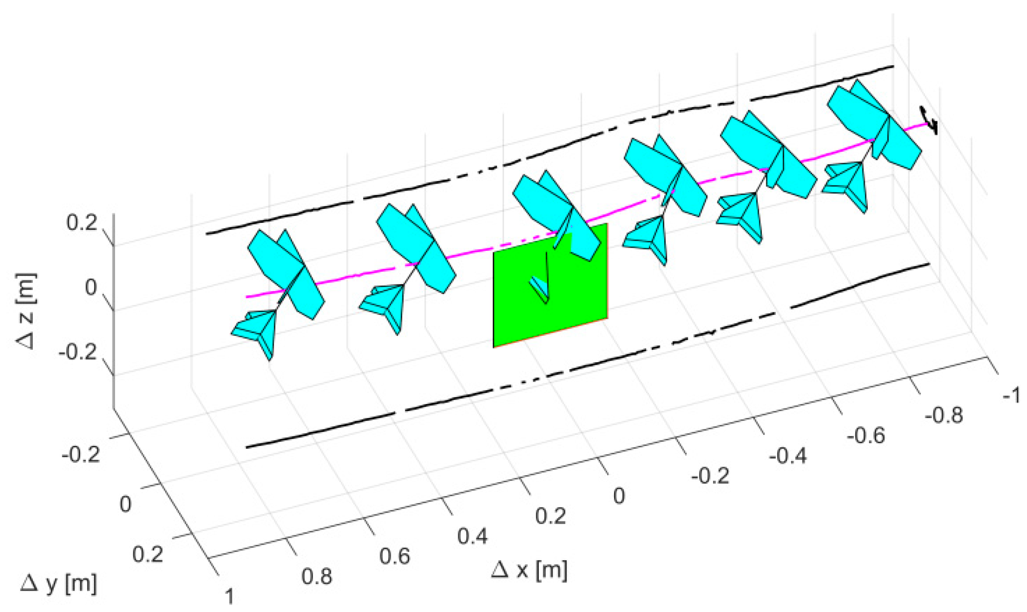
Figure 4.
The DelFly crossing the PIV area, indicated by the green rectangle. The purple line represents the center-of-gravity path and the black lines its projection on the horizontal and vertical planes.
Figure 4.
The DelFly crossing the PIV area, indicated by the green rectangle. The purple line represents the center-of-gravity path and the black lines its projection on the horizontal and vertical planes.

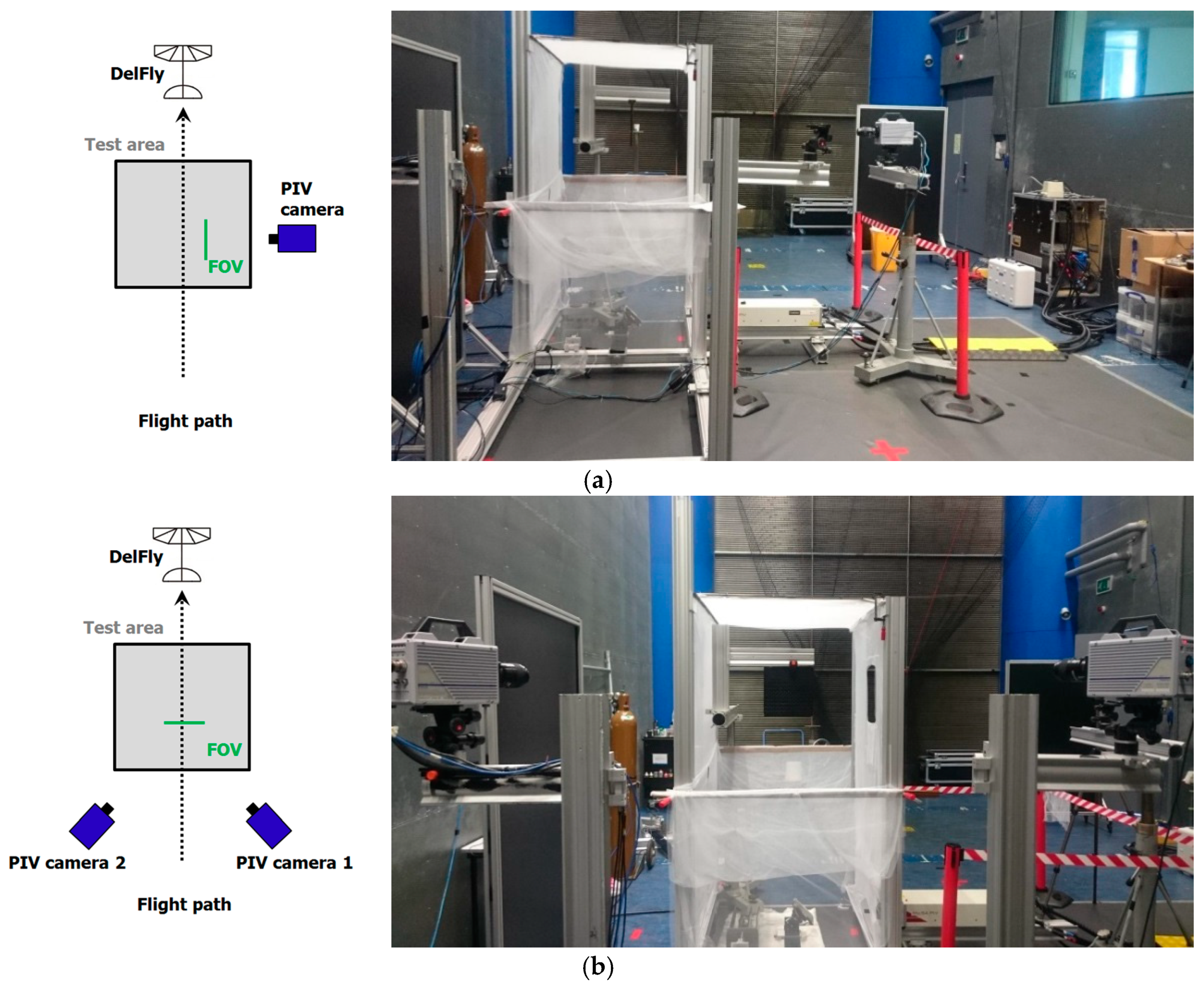
Figure 5.
Experimental configurations for (a) the spanwise flow visualizations and (b) the streamwise flow visualizations. Top view schematic of the test arrangement, not to scale (left) and setup for the PIV measurements (right).
Figure 5.
Experimental configurations for (a) the spanwise flow visualizations and (b) the streamwise flow visualizations. Top view schematic of the test arrangement, not to scale (left) and setup for the PIV measurements (right).

Figure 6.
Contours of out-of-plane vorticity and in-plane velocity vectors during one flapping sequence, for spanwise position S1 (at 45% of semi-wing span).
Figure 6.
Contours of out-of-plane vorticity and in-plane velocity vectors during one flapping sequence, for spanwise position S1 (at 45% of semi-wing span).

Figure 7.
Contours of out-of-plane vorticity and in-plane velocity vectors during one flapping sequence, for spanwise position S2 (at 63% of semi-wing span).
Figure 7.
Contours of out-of-plane vorticity and in-plane velocity vectors during one flapping sequence, for spanwise position S2 (at 63% of semi-wing span).


Figure 8.
Evolution with non-dimensional time t* of the velocity around the DelFly for experiments (S1) and (S2) at different relative probe positions (“inlet” and “outlet”). U and V refer to the horizontal and vertical speed components, respectively. The dashed lines (subscript av) indicate the results phase-averaged over the available flapping sequences.

Figure 9.
Flow conditions perceived by the tail (total airspeed and relative angle of attack) for two different spanwise positions (S1: 45% and S2: 63% of semi-wing span).
Figure 9.
Flow conditions perceived by the tail (total airspeed and relative angle of attack) for two different spanwise positions (S1: 45% and S2: 63% of semi-wing span).

Figure 10.
Contours of out-of-plane vorticity in a spanwise-oriented plane, during one flapping sequence; DelFly model outline is indicative only.
Figure 10.
Contours of out-of-plane vorticity in a spanwise-oriented plane, during one flapping sequence; DelFly model outline is indicative only.


Table 1.
Cycle-averaged velocities.
| Cycle-Averaged U-Velocity | S1 | S2 | Cycle-Averaged V-Velocity | S1 | S2 |
|---|---|---|---|---|---|
| inlet | −0.92 m/s | −0.36 m/s | inlet | −0.05 m/s | −0.33 m/s |
| outlet | −0.45 m/s | −0.97 m/s | outlet | −2.64 m/s | −3.40 m/s |
| outlet-inlet | +0.47 m/s | −0.61 m/s | outlet-inlet | −2.59 m/s | −3.07 m/s |
© 2018 by the authors. Licensee MDPI, Basel, Switzerland. This article is an open access article distributed under the terms and conditions of the Creative Commons Attribution (CC BY) license (http://creativecommons.org/licenses/by/4.0/).
Share and Cite
MDPI and ACS Style
Del Estal Herrero, A.; Percin, M.; Karasek, M.; Van Oudheusden, B. Flow Visualization around a Flapping-Wing Micro Air Vehicle in Free Flight Using Large-Scale PIV. Aerospace 2018, 5, 99. https://doi.org/10.3390/aerospace5040099
AMA Style
Del Estal Herrero A, Percin M, Karasek M, Van Oudheusden B. Flow Visualization around a Flapping-Wing Micro Air Vehicle in Free Flight Using Large-Scale PIV. Aerospace. 2018; 5(4):99. https://doi.org/10.3390/aerospace5040099
Chicago/Turabian StyleDel Estal Herrero, Alejandro, Mustafa Percin, Matej Karasek, and Bas Van Oudheusden. 2018. "Flow Visualization around a Flapping-Wing Micro Air Vehicle in Free Flight Using Large-Scale PIV" Aerospace 5, no. 4: 99. https://doi.org/10.3390/aerospace5040099
Note that from the first issue of 2016, this journal uses article numbers instead of page numbers. See further details here.