1. Introduction
Autonomous Unmanned Aerial Vehicles (UAVs) are increasingly being the focus of several indoor applications requiring higher level of automation. The research community has addressed several autonomous indoor problems such as exploration [
1], search and rescue [
2,
3], and inspection of pen-stocks [
4,
5].
In autonomous indoor missions, the UAVs are required to have capabilities which allow them to navigate in unknown and unstructured environments in presence of several ground obstacles, perceiving the environment and interacting with its diverse components. To successfully execute such kind of missions, UAVs require a proper estimation of its flight altitude, in order to maintain a steady flight when performing the navigation, perception and interaction tasks. In such scenarios, a fast and robust estimation of the UAV flight altitude becomes a critical necessity for autonomous navigation.
Different kinds of techniques have been introduced in the literature for altitude estimation of UAVs in GPS-denied indoor environments using several kinds of sensors such as: laser altimeters, ultrasonic altimeters, barometers, accelerometers (IMU) and vision-based systems. Laser altimeters are very accurate but, in cluttered environment with various ground obstacles, they measure the altitude only with respect to the ground obstacles. The ultrasonic altimeters are similar to the laser altimeters, generally have shorter maximum range as compared to laser altimeters and measure the altitude with respect to the ground obstacles. Hence when directly using the measurements from the laser or the ultrasonic altimeters, it is not possible to measure the accurate flight altitude in presence of a cluttered environment consisting of several ground obstacles.
Barometers measure the altitude from the pressure changes in the environment, but they are very noisy and biased when used indoors and on board the UAVs, due to the ceiling, ground, and wall effects. Accelerometers can be used to provide an estimate of altitude, double integrating the vertical accelerations, but having huge drift in time and bias in its measurements due to the vibrations during a UAV flight.
Computer vision systems based on RGB or RBG-D information provided by the cameras are also widely used for estimating numerous parameters related to the UAV instantaneous state, including the altitude, because they provide more information about the environment at a given time interval as compared to laser altimeters. However, computer vision systems also suffer from several drawbacks: the monocular systems cannot recover the scale from the environment, and stereo based systems are computationally very expensive. Both cases require textured environment which cannot be guaranteed in all indoors scenarios, especially regarding ground surfaces, which are often polished with high light reflectance properties.
In this paper, we propose an algorithm consisting of a 3D point cloud sensor, tilted downwards towards the ground surface, along with an Inertial Measurement Unit (IMU) to robustly and rapidly estimate the flight altitude of UAVs in unstructured, cluttered and dynamic environments, consisting of several ground obstacles and without any requirements of textured surfaces. To summarize, we propose the following main contributions:
Fast 3D planar clustering and horizontal plane segmentation from a 3D point cloud data.
Kalman filter-based mapping of the segmented horizontal planes for accurate flight altitude estimation of UAVs.
Experimental validation of the proposed algorithm in the presence of several static and dynamic obstacles of different shapes and size.
The remaining paper is arranged as follows:
Section 2 presents a detailed related work regarding the state-of-the-art techniques for estimating the altitude of UAVs as well as techniques used for localizing mobile robots using 3D planar surfaces.
Section 3 and
Section 4 describe in detail first, the 3D planar clustering and horizontal plane segmentation method and second, the localization and mapping of these segmented horizontal planes for a robust flight altitude estimation.
Section 5 and
Section 6 present and discuss the experiments and the results obtained when using the IROS 2011 dataset and when performing autonomous real flights using our custom UAV framework, thus validating and demonstrating the usefulness of our proposed approach. Finally,
Section 7 concludes the paper and points out some future work lines.
2. Related Work
The aim of this section is to provide an overview of the current research carried out in the field of UAVs for estimation of the flight altitude using several on-board sensors. Since the presented work in this paper estimates the flight altitude of UAVs using methods related to Simultaneous Localization and Mapping (SLAM) of 3D planar surfaces, we also provide an overview of the current 3D surface-based SLAM algorithms, used for localizing mobile robots.
2.1. Flight Altitude Estimators
2.1.1. Sensor Fusion Based Techniques
This section presents the current research for estimating the flight altitude of the UAVs using several conventional sensors such as laser altimeters, accelerometers, barometers etc. Grzonka et al. [
6] present an autonomous UAV for navigation in indoor environments. They estimate the altitude using a multilevel-SLAM technique for mapping the different level of the ground objects using the measurements from laser beams deflected downwards. Using only 1D laser beam information pointing downwards can have lot of noise in the measurement when flying on top of complex structured obstacles, resulting in wrong mapping of the ground obstacles. The map of the ground obstacles is created depending on the
x-
y-axis position of the UAV and hence altitude estimation is valid only in presence of static ground obstacles and would fail in presence of dynamic ones.
Dryanovski et al. [
7] propose a simple altitude estimation of a UAV deflecting several laser beams downwards, creating a histogram of a certain bin size. After detecting a peak of the histogram (a ground obstacle), a bin is created and an average of the readings belonging to that bin is computed, thus estimating the flight altitude and the height of the ground obstacle present. This approach does not consider the noise in the measurements of a laser neither performs a sensor fusion technique fusing the laser measurements with other sensor measurements.
Szafranski et al. [
8] provide a solution for estimating the UAV altitude fusing the altitude derived from a pressure sensor with an ultrasound sensor. The authors pre-filter the readings coming from both sensors and use a filter to fuse the sensor measurements, based on their assigned weights. The assigned weight for the ultrasound is higher in lower altitudes due to higher accuracy and less for the pressure sensor and vice a versa. At higher altitudes greater than 2–3 m the ultrasound sensor provides noisy measurements of altitude and the filter mostly depends on the pre-filtered altitude provided by the pressure sensor. The authors do not estimate any bias which might be present in the altitude measured by the pressure sensor and they do not compare the estimated altitude with a ground truth system.
Wang et al. [
9] present an autonomous UAV navigation solution for partially known indoors environments, using two 2D laser sensors and an IMU. For the estimation of the altitude, authors use the a 2D laser sensor mounted orthogonally with respect to the UAV. They filter the laser measurements by line segments, where the line segments are sorted based on the perpendicular distance between the ground plane and the center of the laser sensor. The longest line segment is thus assumed to be the flight altitude of the UAV. In presence of ground obstacles, this method only works if the laser sensor projects some beams on to the ground plane. Kumar et al. [
10] present a UAV system with integration of two 2D laser sensors and IMU in industrial environments for real-time pipeline classification. The authors use similar approach for flight altitude estimation presented by [
9], thus suffering from the similar limitations.
2.1.2. Vision Based Techniques
Much research has been carried out estimating the altitude of UAVs using vision-based systems. Cherian et al. [
11] evaluate a machine learning approach for estimating the altitude of a UAV using top-down images from a single on-board camera. The algorithm learns to estimate the altitude by mapping textured information in an image to a possible altitude value, thus it always requires a textured ground surface. It also provides higher errors in presence of ground obstacles.
Eynard et al. [
12] propose a flight altitude estimation of a UAV using mixed stereoscopic vision system consisting of a combination of an omni directional camera with a perspective camera. The authors propose a plane sweeping approach to find a homography between the two views and with the sensor being calibrated and using an estimation of the attitude, estimate the flight altitude of the UAV along with estimating the ground plane. This technique can estimate the accurate flight altitude of a UAV only when the ground plane is present in the image, the more ground obstacles present the less accurate is the estimation of the altitude. The algorithm performs poorly in the presence of poorly texture or homogeneous planes. Mondragón et al. [
13] present a real-time 3D pose estimation of a UAV, along with its altitude, with a single downward looking camera, using planar object tracking. Even though this method uses a single perspective camera for the pose estimation, it requires the use of artificial markers in the environment.
Natraj et al. [
14] evaluate a vision-based system consisting of a fisheye camera and a laser circle projector mounted on a fixed baseline. They provide a theoretical study of a camera modeled as a sphere and to obtain the attitude and the altitude of a UAV estimating a conic on this sphere. This approach assumes that the laser circle projector always projects on to the ground plane, hence does not provide a solution in presence of ground obstacles. Lange et al. [
15] propose an autonomous corridor flight of a UAV using an RGB-D camera to estimate the distances from the walls of the corridors. The authors use a SRF10 sonar sensor for measuring the altitude of UAV and 3D planar information from an RGB-D camera only for keeping the UAV aligned in the center of the corridor. The authors do not provide any solution for altitude estimation of the UAV in presence of ground obstacles, performing the experiments in corridors without ground obstacles.
Shen et al. [
16] address a development of a vision-based system for state estimation and trajectory control for a high-speed UAV flight, consisting of two fisheye cameras along with an IMU, to estimate the orientation as well as the 3D position of the UAV, using a Visual Inertial Navigation System (VINS)-based estimator. As the system depends on the features extracted from the environment, repetitive patterns or featureless scenarios cause drift in the estimated altitude of the UAV.
Boutteau et al. [
17] propose a system based on circular laser source and an RGB camera for estimating the attitude and altitude of a UAV. The authors develop a geometric modeling to estimate the pose at the scale of the system and relative to the plane onto which the pattern is projected, unable to estimate the correct altitude in presence of ground obstacles. Chirarattananon [
18] propose an altitude estimation of UAVs combining the direct optic flow measurements from a single camera with the measurements from an IMU, but the author does not evaluate the performance of the algorithm in presence of ground obstacles.
2.2. 3D Surface-Based Localization
The research community has witnessed several algorithms based on 3D planar localization and mapping techniques applied mostly to ground robots. de la Puente et al. [
19] describe a 3D mapping approach based on compact models of semi-structured environments in partially destroyed buildings, for carrying out rescue work using ground robots. The authors use 3D data from a laser scanner along with computer vision techniques to segment 3D surfaces, not necessarily planar. A maximum incremental probability algorithm based on Extended Kalman Filter (EKF) provides 6D localization and produces a map using the planar patches with a convex hull-based representation.
Cupec et al. [
20] introduce a fast pose tracking algorithm based on planar segments extracted from range images applied to a ground robot. The algorithm consists of an EKF-based directed search hypothesis algorithm using a tree structure estimating the pose of the robot. The authors test the algorithm offline using a pre-collected dataset of RGB-D images.
Biswas and Veloso [
21] also perform a depth camera-based indoor localization of a ground robot on a pre-generated map of the environment. The authors extract the planar segments and their corresponding normals from the point clouds, downsample the plane filtered points to 2D lines and match them with the existing 2D map for localization. Although the authors provide very good localization results, their approach is limited to environments with a known map.
As can be noted from
Section 2.1, robust flight altitude estimation of UAVs in cluttered, dynamic, and unknown environments with ground obstacles, remains an open problem. In our previous work [
22], we addressed this problem, estimating the flight altitude of a UAV along with the height of the ground obstacles using an EKF-based sensor fusion technique, fusing the measurements from a laser altimeter, barometer, and vertical accelerations from an accelerometer. Nevertheless, due to the limitation of the laser altimeter, measuring the distance with respect to ground obstacles only at a single point at a given time interval, the estimation of the ground obstacle height was limited to be one dimensional instead of a 3D plane. This caused errors in the height estimation of the ground obstacles in presence of highly complex structures of the ground obstacles thus increasing the errors in the estimated flight altitude.
To improve the limitations of the previous works and taking into account the advantages of the previously mentioned 3D surface-based localization techniques which can provide enhanced information of the ground obstacles, we propose an innovative approach using 3D point cloud data, for accurately estimating the height of the ground obstacles and the flight altitude of the UAVs even in texture-less environments and in presence of several unstructured and dynamic ground obstacles.
3. 3D Planar Clustering and Horizontal Plane Segmentation
In an indoor flight, normally, the flight altitude of a UAV is required to be computed with respect to the ground plane, where the world frame is located on the ground at the take-off point. The obtained 3D point cloud information from a 3D sensor, can be used to extract the 3D surface information of the objects present in the environment. Hence, a 3D point cloud sensor partially inclined downwards, can detect the ground surface as the most prominent 3D planar horizontal surface. Clustering the 3D points relevant to the ground surface and segmenting the 3D planar information can provide us with an estimate of the flight altitude of the UAV with respect to the ground surface.
In presence of ground obstacles, the prominence of the ground surface decreases due to occlusions. In cases of the ground surface being completely occluded, the estimated flight altitude will be inaccurate, as it will be relative the ground obstacle, occluding the ground surface. In order to overcome this problem, we propose to first cluster and segment all the horizontal planes present at a given time instant. Then, we continuously map the segmented planes in order to accurately estimate the flight altitude of the UAV.
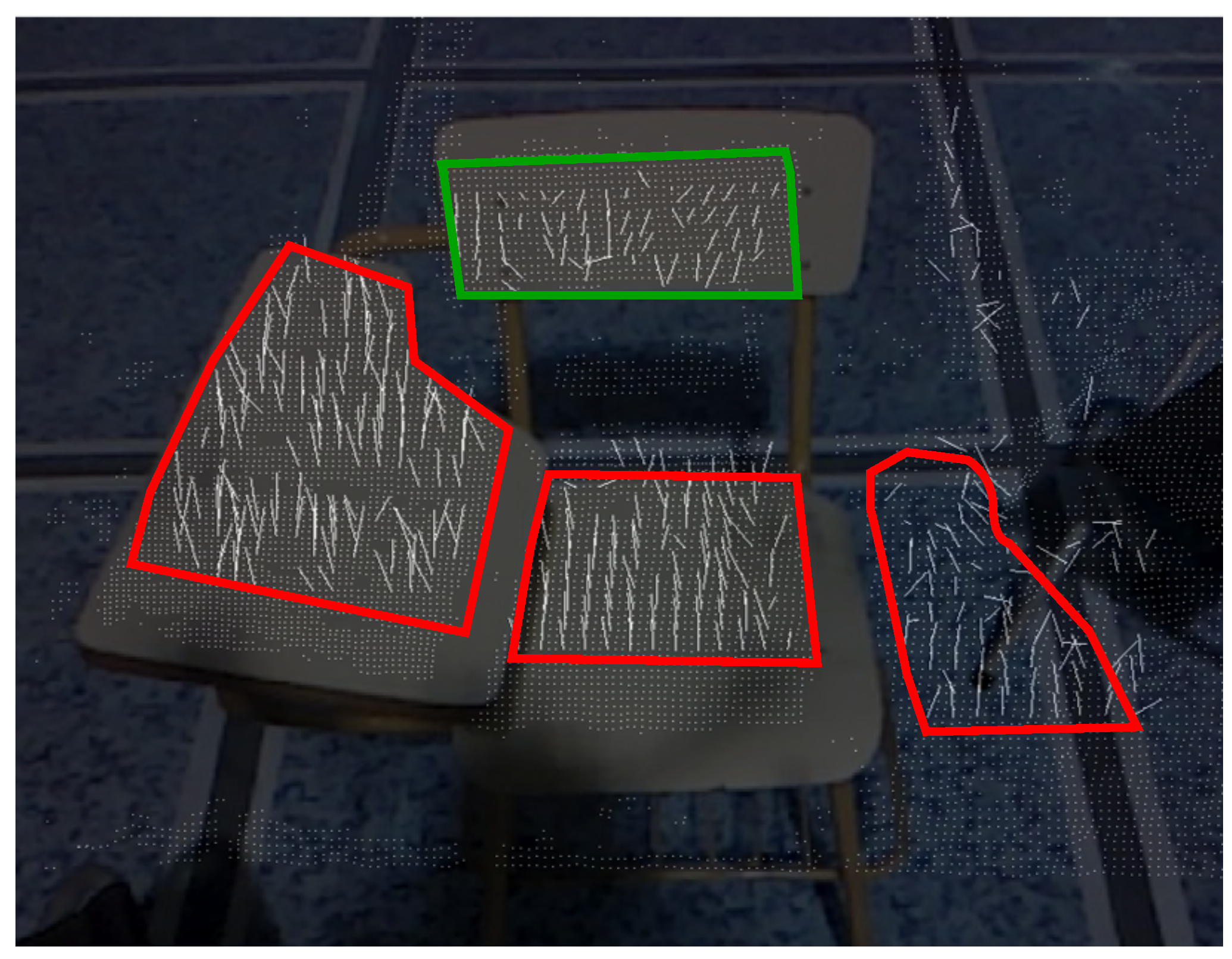
3.1. Normal Based Clustering
In order to cluster 3D planar surfaces, first we compute the point normals at each 3D point. We use the integral image normal estimation technique as explained in [
23], for fast and real-time normal estimation.
An integral image of an image is the sum of all values of within a particular region . In brief, this technique first converts the z-component of the point cloud into an integral image, thus requiring an organized 3D point cloud. This reduces the computation cost and makes it independent of the size of the smoothing windows used to reduce the noise in the 3D point cloud data. A smoothing is then performed choosing appropriate smoothening areas calculated using depth change maps. The normal at a point is then calculated as the cross product of two vectors: , where is a vector between 3D right and left neighbors of the point and is a vector between 3D upper and lower neighbors of point , in the organized point cloud.
The orientation of these computed normals is used for the clustering all the 3D planes present in the environment. We cluster all the computed normals using a
K-means clustering algorithm, which provides the normal centroids of all the present 3D planes including all the horizontal planes. These clustered centroids of the normals constitute the matrix
.
Figure 1 shows an example containing a ground obstacle with all the computed normals with their orientations and their respective clusters.
3.2. Horizontal Plane Segmentation
As shown in
Figure 2, the normal centroids computed from the above-mentioned
Section 3.1 are with respect to the sensor frame of reference
. In accordance to the definition of the world reference system, the normals of the horizontal planes are always parallel with respect to the
z-axis of the world reference frame, which is used for segmenting the horizontal planes. Converting all the normal centroids from sensor frame to world frame becomes a computationally expensive and time-consuming process. In order to speed up the computation, instead of converting all the computed normal centroids to the world frame, we convert the orientation of a single horizontal ground plane normal in the world frame, which is always known and fixed, into the sensor frame as:
being the transformation of the sensor frame
to the world frame
.
is a composition of the transformation the of sensor frame
to robot frame
given by
and transformation of the robot frame
to world frame
given by
:
The computed normal centroids of the 3D planes, comprising the matrix
from
Section 3.1, are compared with computed horizontal ground plane normal in the sensor frame,
from Equation (
1). Using a given threshold, the normal centroid of the horizontal planes present in the normals matrix
is segmented. From this segmented normals, all their corresponding 3D points of all the horizontal planes are segmented.
The segmented 3D points along with ground plane normal in the sensor frame
, are used for computing the vertical height of the segmented horizontal planes with respect to the sensor as follows:
where
is a 3D point composed of
in Cartesian coordinates of
x,
y, and
z axis respectively and
composed of the three components
.
A second
K-means algorithm is used for clustering the height vector
, which is a vector of all the computed heights
h from Equation (
3). The height centroids obtained from the second
K-means clustering are used by the localization and mapping stage as explained in the following
Section 4, in order to accurately estimate the flight altitude of the UAV. Algorithm 1 explains briefly the implementation of this section.
| Algorithm 1: 3D Planar Clustering and Horizontal Plane Segmentation. |
![Aerospace 05 00094 i001]() |
4. Horizontal Plane-Based Localization and Mapping
In order to deal with the problem of multiple horizontal planes, we formulate a Kalman filter based localization method to estimate the flight altitude of the UAV based on mapping all the segmented horizontal planes for generating a complete map.
We consider a Kalman filter with the state , comprising of aerial robot state component . It consists of a noise comprising of the robot’s process model noise . The aerial robot state consists of a single component given as:
4.1. Process Model
The discrete time process model of the robot’s estimated height can be given as:
where
is the Gaussian white noise in the vertical component process model and is the only component of the robot’s process model noise
.
4.2. Prediction Stage
The prediction stage follows the standard Kalman filter equations, where the state
x is estimated in the current time instant
k, using the previous estimate at time
.
where
and
are the process and noise variance.
4.3. Measurement Model
The height centroids obtained from the horizontal plane segmentation explained in
Section 3, form the vector of measurements
as:
And its measurement model
being:
4.4. Data Association and Update Stage
The estimated horizontal plane centroids from Equation (
7), are compared with the ones already in the map vector
by means of the Mahalanobis distance. It is assumed that the ground plane is always present at the lowest location of the map, in the world reference frame. Hence the map vector
, initially contains at least the ground plane as a horizontal plane with height zero. For a given measurement
, the measurement innovation is computed as:
where
i ranges from 1 to
m, and
m being the number of map elements in
. The associated innovation variance can be given as:
where
is the associated variance of the current plane measurement
.
The Mahalonobis distances, between the map elements and current measurement are computed as:
All the distances within the given chi-square threshold are sorted in order to obtain the minimum value, and thus the corresponding map element. This selected map element is then associated with the measurement .
If all the computed Mahalonobis distances are above the given threshold, the plane element is added as a new map element.
All the
n matched plane elements at a given time instance, constitute the innovation vector
as well as the noise covariance matrix
. Thus, the new innovation covariance matrix given as:
where
is the Jacobian of the measurement model of the extracted planes with respect to the state
x.
in our case is a column vector, with all elements equal to 1.
After which, the near optimal Kalman gain
is calculated as:
Finally, the corrected values of the state and its covariance are obtained by:
Algorithm 2 provides a summary of the above explained process.
| Algorithm 2: Horizontal Plane-based Localization and Mapping. |
![Aerospace 05 00094 i002]() |
5. Experiments and Results
5.1. Standard Datasets
In order to evaluate and validate our approach, we first test it with a standard dataset provided by the research community, estimating the camera altitude using the provided point cloud data.
5.1.1. IROS 2011 Kinect Dataset
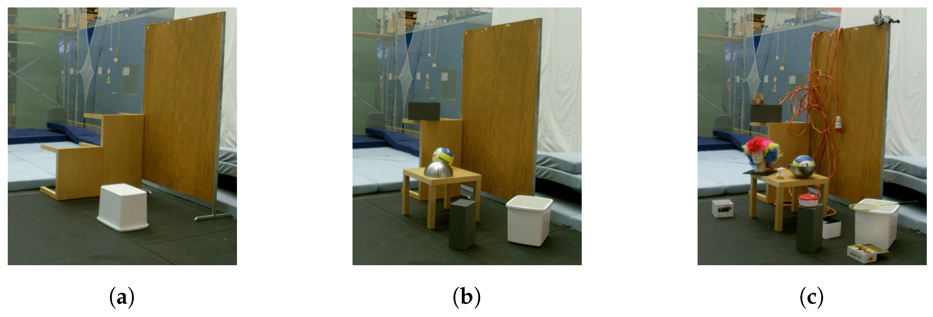
This dataset (
http://projects.asl.ethz.ch/datasets/doku.php?id=kinect:iros2011kinect) consists of point cloud data obtained from a Kinect sensor (Microsoft, Redmond, WA, USA) and ground truth data from a Motion Capture (MoCap) system (Vicon Motion Systems, Oxford, UK) in indoor environment. The data is captured in three distinct indoor environments with increasing complexity of ground obstacles (see
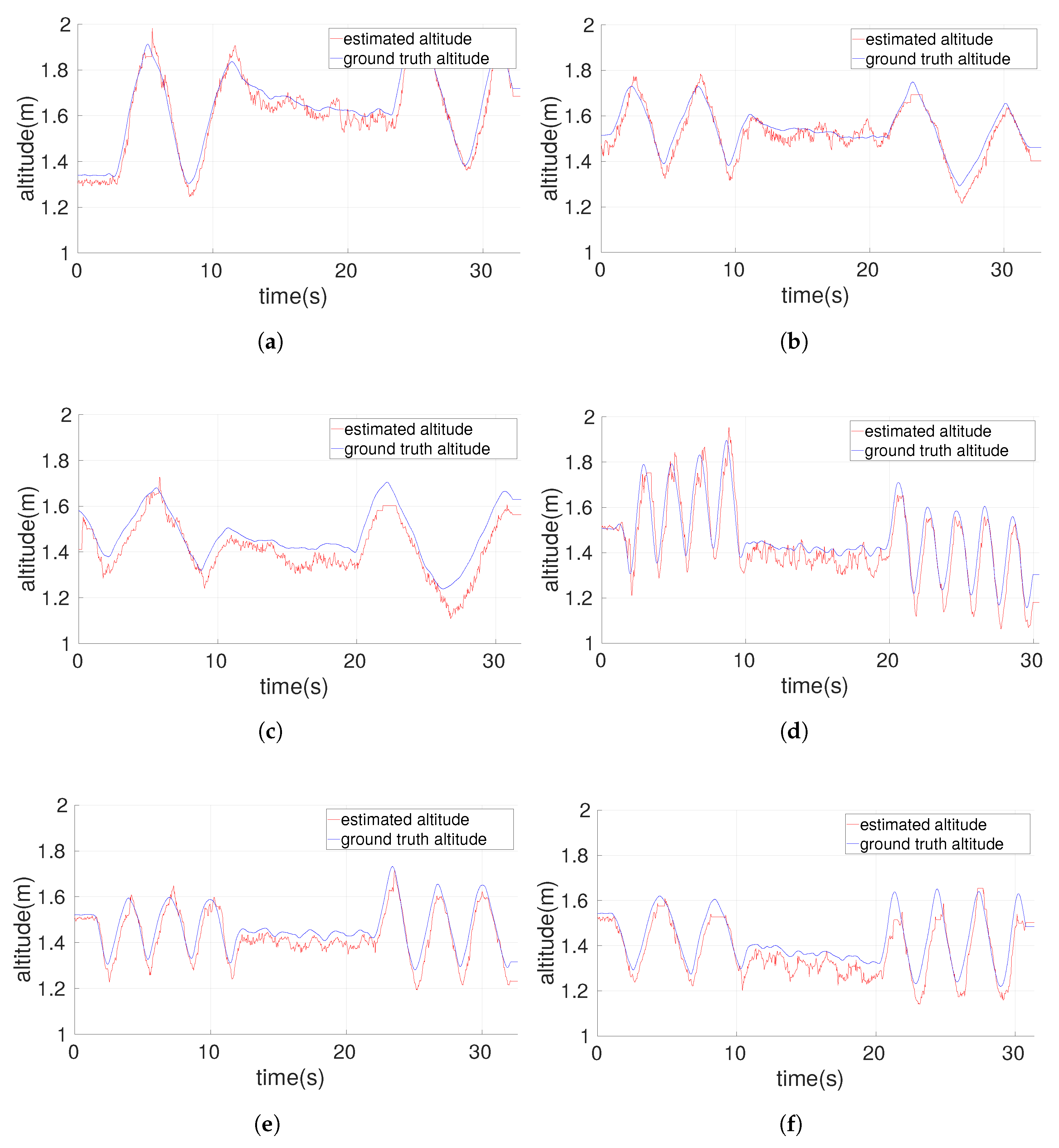
Figure 3) and with three different types of motion performed in slow, medium and fast speeds.
We provide the results for the translation motion of the camera, applied at all three mentioned speeds in low, medium and high complexity ground obstacles. The data consists of 3D point cloud of resolution
at 30 Hz and provides a transformation between the camera frame and the world frame, with our algorithm running at the same frequency of the point cloud data acquisition (30 Hz). For these experiments, we choose initial clusters in both the
K-means algorithms mentioned in
Section 3 based on experimental trials and assign it a numerical value of 3.
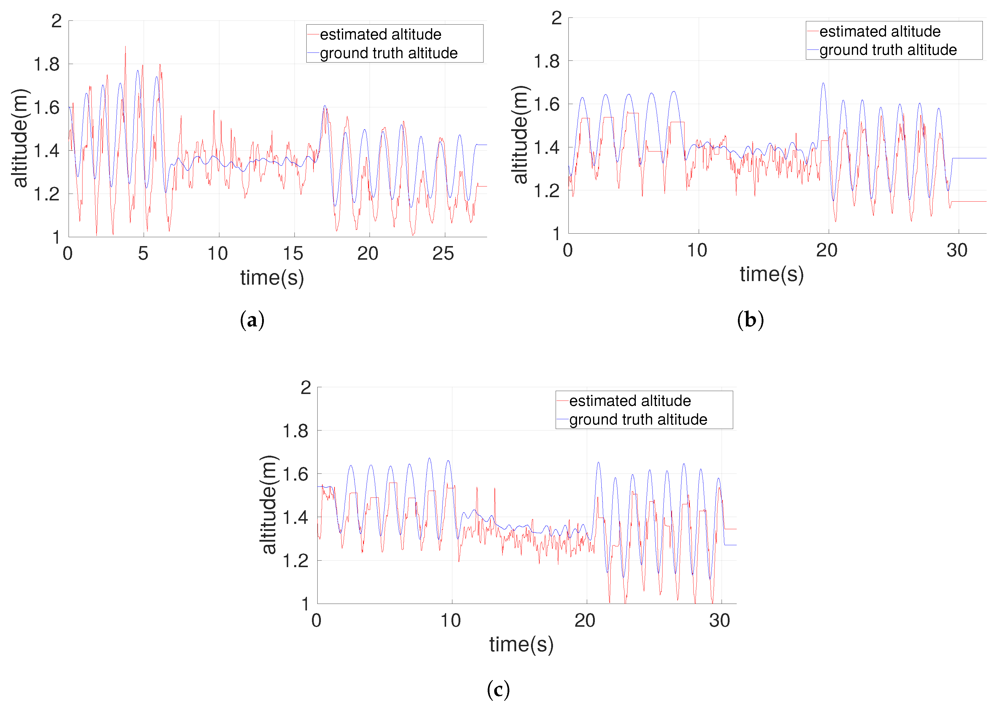
Figure 4 and
Figure 5 elaborate the results of our algorithm in terms of graphs comparing it with the ground truth altitude information obtained from the MoCap system.
Figure 4a–c describe the plots obtained during a slow motion of the camera in low, medium and high complexity environments respectively. The algorithm performs robustly in slow motion even in the presence of hight level of complexity of cluttered environment achieving an average RMSE of
m. Increasing the speed of the translation motion of the camera decreases the accuracy of the algorithm, with the medium speed motions (see
Figure 4d–f) achieving an average RMSE of
m. Whereas the high-speed motion of the camera results in an average RMSE of
m as seen in
Figure 5a–c.
Table 1 represents the individual RMS errors obtained during the execution of each experiment.
5.2. Real Flights
Video link of the performed experiments can be found in
Supplementary Materials. The aim of the real flight experiments, on one hand is to evaluate the capabilities of our proposed approach in presence of unknown, cluttered and dynamic ground obstacles, and on the other hand, to evaluate robustness of the estimation with fast and rapid UAV movements.
Section 5.2.1 explains briefly the setup of our UAV system as well as the configuration of the indoors real flight scenario. After which,
Section 5.2.2 presents the results obtained during the performed autonomous indoor missions.
5.2.1. Experimental Setup
System Setup
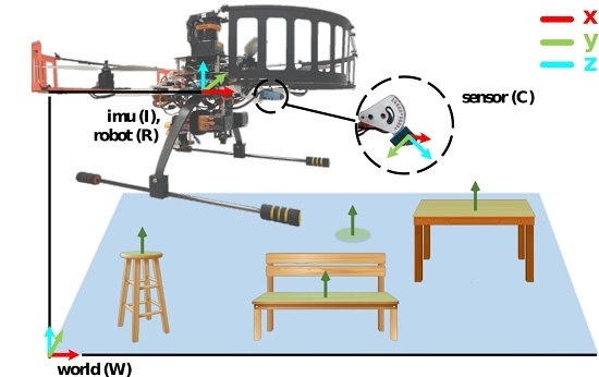
Figure 2 shows the custom UAV platform, used for validating the proposed algorithm. The autopilot used for low level control (attitude control) is Pixhawk (3D Robotics, Berkeley, CA, USA,
https://pixhawk.org/). The Pixhawk consists of an integrated IMU sensor, providing the angular velocities and linear accelerations in all 3-axis. We use on board a Intel RealSense Z200 RGB-D (Intel, Santa Clara, CA, USA,
https://software.intel.com/en-us/articles/realsense-r200-camera) camera for real-time computation of the 3D point cloud. The RGB-D camera is placed at a fixed angle of
deg with respect to the
y-axis of the robot frame, not pointing perpendicular to the ground surface in order that the camera can be used for other future autonomous mission tasks such as object detection, avoiding the need for a dedicated sensor for altitude estimation task. All the computation is carried on board the UAV on an Intel-NUC 6i5SYK mini-compute.
We use an Optitrack MoCap system (Optitrack, Corvallis, OR, USA,
http://optitrack.com/), providing the ground truth flight altitude of the UAV, in order to compare and evaluate our estimated flight altitude. An on-board Lightware SF/10 laser altimeter (Lightware Optoelectronics, Gauteng, South Africa) is also used, only to demonstrate its inaccuracies in presence of ground obstacles.
The software modules were developed in C++ and Robot Operation System (ROS) (Willow Garage, Standford, CA, USA). For a complete autonomous flight the Aerostack architecture (
http://www.aerostack.org) is used, integrating our newly developed software modules of the proposed altitude estimation approach. A full description of the Aerostack architecture can be found at [
2].
Real Flight Configuration
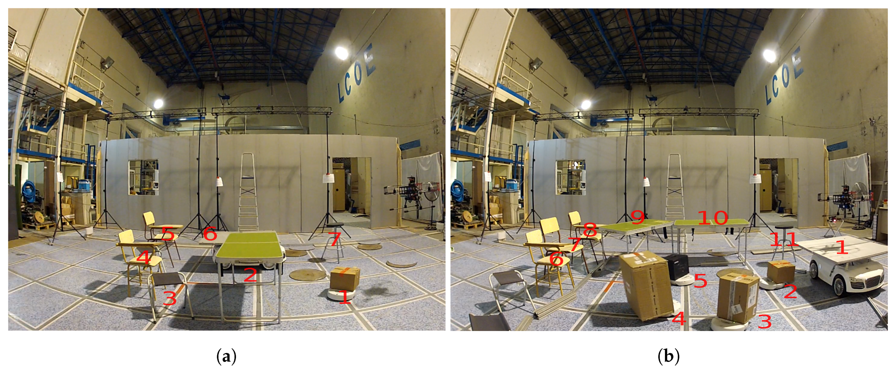
Several autonomous flights were performed in different challenging scenarios in order to validate our approach as shown in
Figure 6.
Navigation in unknown and unstructured indoor environment: (see
Figure 6a) This configuration consists of an indoor area 4 m × 4 m in dimensions. The environment includes several static ground obstacles, with their height lower than the flight altitude of the UAV, placed in an unknown and random manner. The ground obstacles include several chairs with random discontinuity in their surface as well as tables and other objects with uniform surfaces. It also consists of a static iRobot (iRobot, Bedford, MA, USA,
http://www.irobot.com/About-iRobot/STEM/Create-2.aspx) with a box on top as a ground obstacle.
Take-off and land on a platform and navigation in dynamic, unknown and unstructured indoor environments: (see
Figure 6b) Similar to the previous evaluation scenario, this configuration consists of an indoor area 4 m × 4 m in dimensions, consisting of several static as well as dynamic ground obstacles. The static ground obstacles are the same as mentioned in the previous configuration. In order to increase the complexity, we add several dynamic and random ground obstacles, placing different boxes of varying shapes and height on top of iRobots. The iRobots move in a complete random and unknown manner, thus providing random dynamic obstacles. The UAV takes-off and lands on a platform of height
m and area
m
, further increasing the complexity of the mission.
5.2.2. Results
In this section we present the results obtained from performing autonomous flights in the previously mentioned scenarios. The navigation controller uses as feedback the flight altitude estimated by the proposed algorithm.
The UAV is always commanded to maintain a constant flight altitude of
m. The flight altitude estimation is performed at an average real-time frequency of 54 Hz, with the point cloud being received at 60 Hz. The point cloud resolution being 160 × 120. In all the experiments, the UAV performs an autonomous but pre-defined squared trajectory over the mentioned area. The initial clusters in both the
K-means algorithms mentioned in
Section 3 are chosen through experimental evaluations and assigned a numerical value of 3. The squared trajectory is performed twice, in order to validate the performance of the mapping stage of our proposed algorithm as explained in
Section 4.
Navigation in unknown and unstructured indoor environment: In this experiment, the UAV performs the autonomous squared trajectory with two different velocities, one at lower velocity of m/s and the other at a higher velocity of m/s in the static ground obstacles environment.
- -
Low Velocity Flight:Figure 7a represents the results of the low velocity (
m/s) autonomous flight of the UAV. It can be seen from
Figure 7a, when comparing the estimated altitude with the ground truth altitude we get an RMS error of
m.
- -
High Velocity Flight:Figure 7b represents the results obtained from the high velocity autonomous flight of the UAV. The RMS error achieved is
m, when compared to the ground truth altitude.
Take-off and land on a platform and navigation in dynamic, unknown and unstructured indoor environments: In these experiments, we perform autonomous low ( m/s) as well as high (1 m/s) velocity UAV trajectories in dynamic and unstructured environment. The UAV takes-off and lands on a platform and as the height of a platform is well known, we pre-define the initial height of the UAV as the height of the platform. The initial map of the horizontal height centroids contains the height of the platform plane along with the ground plane.
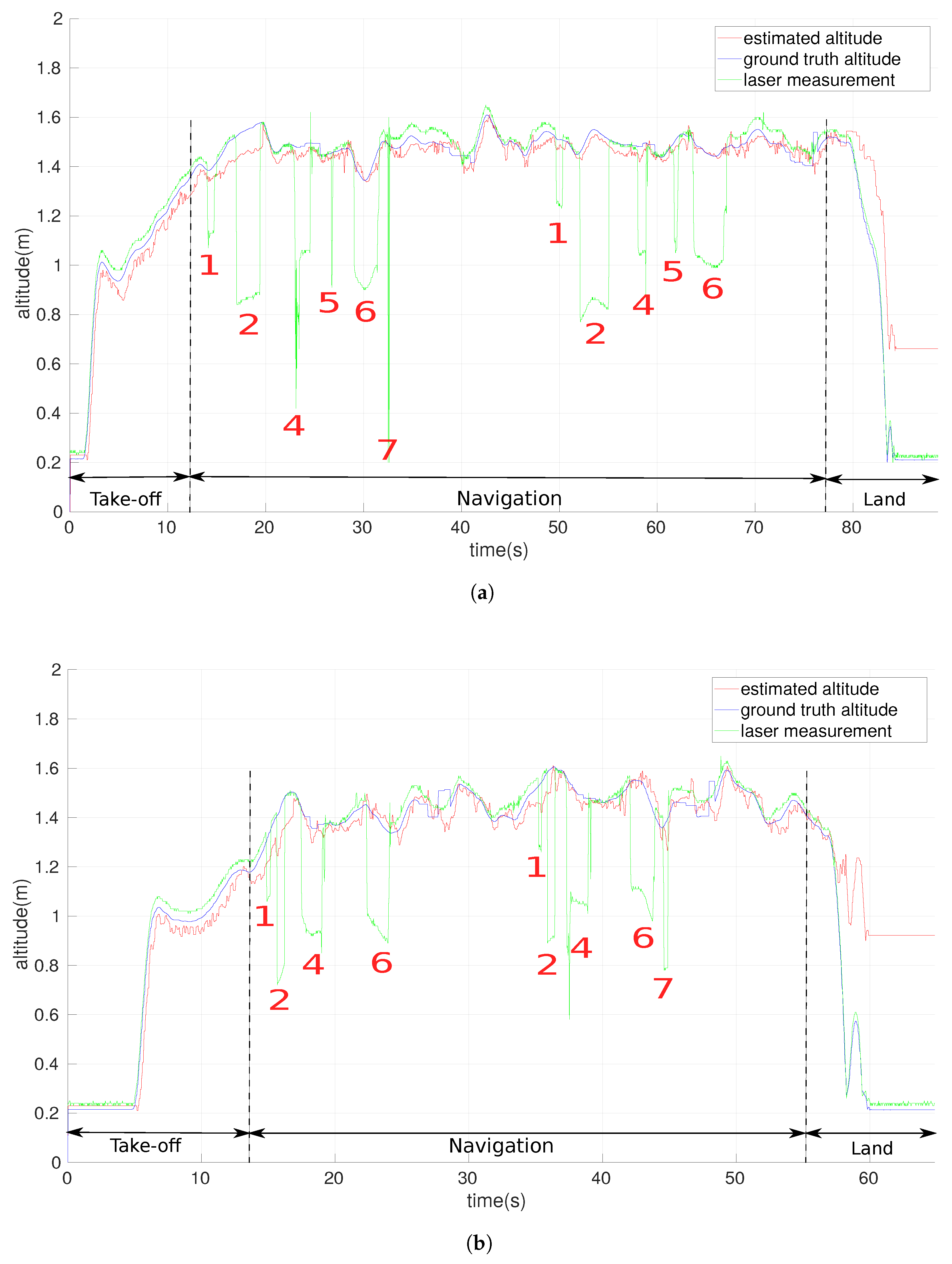
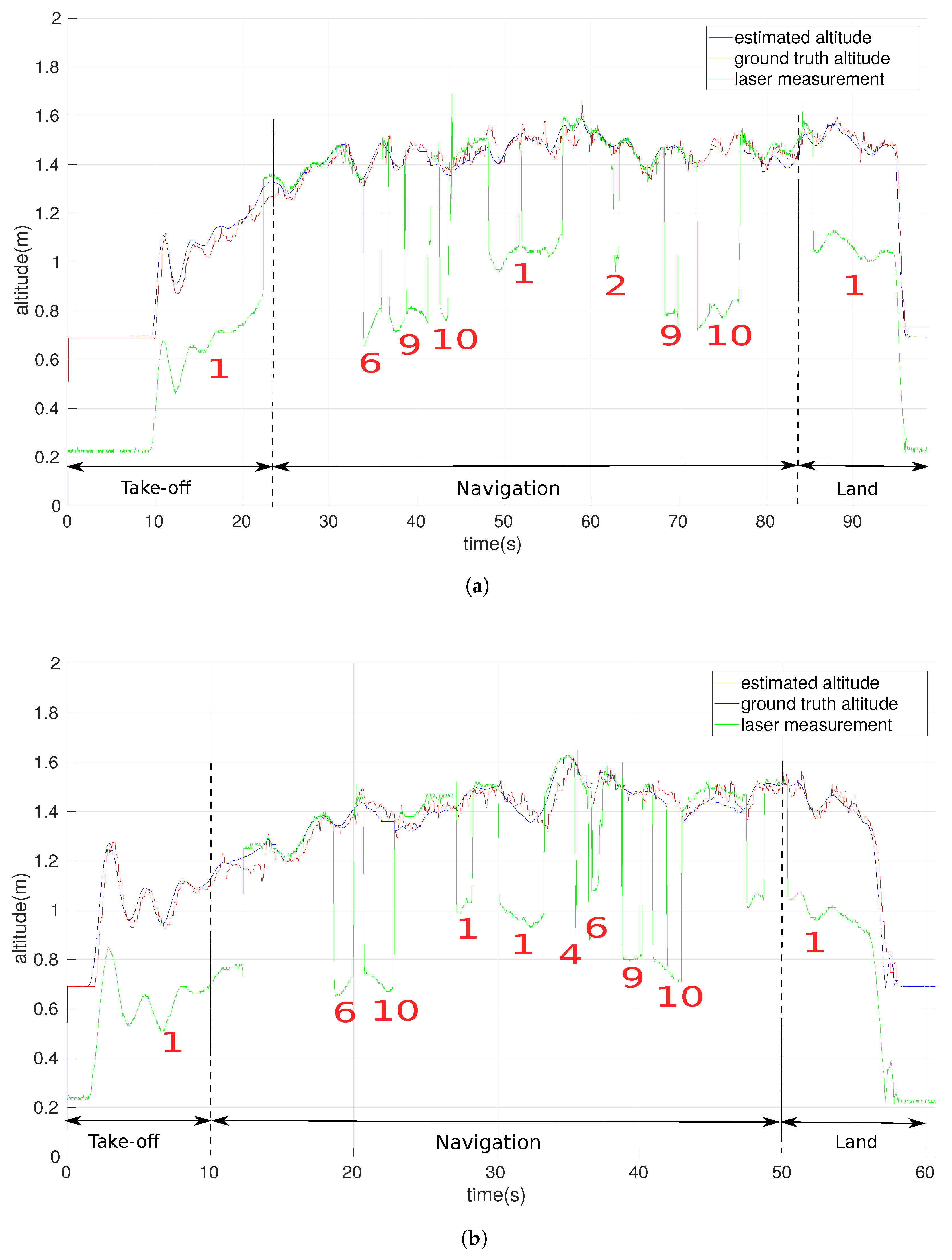
- -
Low velocity flight:Figure 8a represents the results obtained during the low velocity flight of
m/s. As it can be seen from the figure, during the take-off phase (
t = 0 s to
t = 22 s) the altitude measured by the laser altimeter is inaccurate as it is with respect to the platform. Whereas the altitude estimated by our algorithm is accurate even though the ground plane is not detected most of the time during this phase. After the take-off phase the UAV navigates through the dynamic environment (see time
t = 22 to
t = 85 in
Figure 8a), consisting of several moving ground obstacles as well as static ground obstacles. We achieve an RMS error of
during this proposed experiment.
- -
High velocity flight: Similar to the previously mentioned low velocity experiment, we perform the autonomous mission at a higher velocity of 1 m/s. We achieve an RMS error of m when comparing the estimated altitude with the ground truth altitude.
6. Discussion
6.1. Standard Datasets
As presented in
Section 5.1 our algorithm accurately estimates the correct camera altitude with very low RMS error, as it correctly segments and maps the horizontal planes, in presence of several ground obstacles irrespective of the complexity of their shape and size (see
Figure 4a–f and
Table 1) at slow as well as medium speed camera translation motions. During high-speed camera translation motions, at several time instances, there is absence of horizontal planes in the point cloud data adding errors in the estimation (for example in
Figure 5c between time instances
t = 0 to
t = 10). Nevertheless, as the algorithm maps all the horizontal planes (
Section 4), it recovers the correct altitude estimation when the horizontal planes appear again in the point cloud data, matching them appropriately with the already mapped planes.
In the experiments, the camera motion is performed in a completely random manner and the new ground obstacles added for complexity are non-planer, smaller in size just occluding to some amount the present horizontal planes, thus they neither increase or decrease the accuracy of the algorithm. Because of the above reasons within a given speed of the camera the RMS errors do not follow a pattern (see
Table 1), and are based on the random translation motions performed. But it can be clearly seen from
Table 1, as the speed of these translation motions increases, the RMS errors increase as well due to the fact that at high speeds during several time instances the horizontal planes are absent in the point cloud data.
6.2. Real Flights
As it can be seen from the
Section 5.2.2, our algorithm performs quite robustly in presence of high complexity-shaped dynamic and static ground obstacles, as well as with high-speed movements of the UAV. It can be appreciated from
Figure 7a,b with low as well as high velocities of
m/s and 1 m/s, our proposed algorithm efficiently estimates the flight altitude when comparing it with the ground truth altitude.
It can be seen from
Figure 7a between time instances
t = 20 s and
t = 30 s and time instances
t = 30 s and
t = 40 s, that the laser altimeter measurements have several peaks which are caused due to obstacles number 4 and 7. Obstacle number 4 is a chair with an asymmetric shape which causes the laser measurements to get deflected causing such peaks. Whereas in case of obstacle number 7 due to the speed of the UAV, laser gets deflected at the edge of the obstacle causing such large peak. Due to these errors in the measurements, laser altimeter measurements cannot be directly used for closing the altitude control loop of the UAV. A heuristic approach for calculating the flight altitude of the UAVs, based on filtering the laser measurements can accumulate large errors and hence would not work accurately in presence of such obstacles as well. Whereas in our proposed approach, as we segment and map the 3D horizontal planes, the complexity of the shape of the ground obstacles does not affect the accuracy of the flight altitude estimate of the UAV as seen from
Figure 7a,b.
These laser measurement errors can also be seen in
Figure 7b between time instance
t = 30 s and
t = 40 s as the laser measurements are deflected by the obstacle number 4, and estimation from our proposed approach remains unaffected.
The flight altitude estimation in presence of dynamic obstacles can be appreciated from
Figure 8a,b. During the take-off phase in presence of obstacle number 1, the laser measurements are with respect to the obstacle 1 whereas our algorithm having the input height of the obstacle 1, estimates the correct flight altitude of the UAV during the entire take-off phase. During the entire navigation stage due to the presence of several random moving dynamic as well as static obstacles, several laser measurements get referred to the obstacles instead of the ground, making it impossible to use such measurements for estimating the flight altitude fo the UAV. As our approach rapidly maps all the present horizontal planes, it can accurately estimate the flight altitude of the UAV in such environment at both slow as well as high UAV velocities of
m/s and 1 m/s respectively. It can also be appreciated from
Figure 8a,b that as our algorithm maps and localizes based on all the present horizontal planes, random and dynamic nature of the ground obstacles has no effect on the performance of our algorithm.
It can seen from
Section 5.2.2 that the average RMS errors in presence of dynamic obstacles is less as compared to static obstacles, this is because in the dynamic scenario the number of ground obstacles with horizontal planes is greater as compared to static scenario. Higher number of ground obstacles thus provide higher number of horizontal planes for the localization and mapping stage (
Section 4), improving the accuracy of the algorithm. Even though the obstacles have dynamic random motion, our algorithm maps them based on their horizontal plane height and matches them accurately when they are re-encountered, making it robust against dynamic motion of the ground obstacles, and thus improving the accuracy of the estimated flight altitude of the UAV.
It should be noted that even though in all the performed experiments the commanded flight altitude is kept constant to m in order to compare the algorithm with the ground truth data and the laser measurements, our algorithm can perform equally at different commanded flight altitudes during the execution of the mission, provided that the commanded altitudes are within the minimum and maximum ranges of the point cloud sensor.
6.3. Limitations
Our proposed approach currently faces a limitation that, during the absence of any horizontal plane, the estimated flight altitude can have inaccuracies. These errors can be resolved fusing more sensors such as accelerometers, barometers etc., as presented in [
22]. As this research is focused on presenting the flight altitude estimation results of a UAV using point cloud sensors, we currently do not fuse other sensor measurements.
This limitation can be clearly pointed out in the
Section 5.1.1, while performing very fast camera motions, the computed point cloud lacks information of any horizontal plane, during several time instances. This can be observed in
Figure 5c, between time instance
t = 0 s and
t = 10 s. During such time instances, the Kalman filter in our proposed approach, propagates the state using the constant velocity noise model (see
Section 4). This causes the increase in the RMS error with increasing motion of the camera, whereas the complexity of ground obstacles in the environment does not affect the accuracy our proposed approach. This limitation can also be pointed out in real flight experiments from
Figure 7a,b, as the estimated altitude during the landing phase is not accurately estimated when compared with the ground truth altitude. This is because during the landing phase the Intel RealSense sensor is very close to ground surface, unable to provide any reliable point cloud information and hence no horizontal plane is extracted.
Even though suffering from this above-mentioned limitation, in a real UAV flight with RGB-D camera on board the UAV, inclined downwards and with fast UAV motions up to 1 m/s, the computed point cloud always contains at least one horizontal plane. In addition, as we map all the horizontal planes, the performance of our proposed approach is not affected when testing with real and fast UAV flights except during the landing phase, which usually does not affect performance the autonomous mission, as it being the last and concluding phase of the mission (see
Section 5.2.2).
Our proposed approach can map the ground obstacles only below the flying altitude of the UAV. With the current sensor setup of our UAV used in the experiments, if there is a ground obstacle taller than the flight altitude, it will be discarded by our algorithm as no horizontal plane would be detected. Whereas such ground obstacles would be detected and avoided using the 2D laser sensor on board the UAV. Obstacle detection and avoidance using the 2D laser can be found in our previous work [
24].
7. Conclusions and Future Work
In this paper, we present a fast and robust point cloud-based altimeter, accurately estimating the flight altitude of UAVs, in presence of several static as well as dynamic ground obstacles, in indoors environment.
Our proposed approach is based on fast segmentation of 3D planar surfaces from a 3D point cloud data computed from any point cloud sensor. We cluster the obtained 3D planar surfaces in order to segment the 3D horizontal planar surfaces. We map the vertical distances of the 3D horizontal planar surfaces, in order to provide a robust estimation of the flight altitude of the UAV. Our algorithm works at a fast real-time frequency of 54 Hz, with the point cloud acquisition frequency of 60 Hz.
Several experiments have been performed in order to validate our approach. We first compare our results with IROS 2011 standard Kinect dataset obtaining very low RMS errors when compared to the ground truth data. We also perform several real indoors flights in presence of several static as well as dynamic obstacles, achieving an RMS error as low as m, when comparing it with the ground truth data.
We also release our work as an open-source software within our Aerostack framework (
www.aerostack.org), for the research community to benefit for their experiments.
An immediate line of future work is to robustly estimate the x-axis and y-axis position of a UAV along with the robust flight altitude estimation using the point cloud sensors, in dynamic and unstructured indoors environment. Since obtained the point cloud, is generally very noisy in the x-axis and y-axis direction, segmenting 3D planar surfaces in these directions and achieving robust localization becomes a challenging tasks. As a second line of future work, we plan to improve the data association problem, when matching segmented planes, for a more accurate mapping stage and thus an even more robust localization.

 ,
, 


