Modelling Airport Pollutants Dispersion at High Resolution ^†

Abstract

Local air quality is a major concern for the population regularly exposed to high levels of air pollution. Due mainly to its aircraft engine activities during taxiing and take-off, the airport is often submitted to heterogeneous but important concentrations of NO${}_x$ and Particulate Matter (PM). The study suggests an innovative approach to determining the air traffic impact on air quality at the scale of the airport, its runways, and its terminals, to be able to locate the persistent high-concentration spots, for example. The pollutant concentrations at 10 m resolution and 1 s time step are calculated in order to identify the most affected areas of an airport platform and their contributors. A real day of air traffic on a regional airport is simulated, using observations and aircraft trajectories data from radar streams. In order to estimate the aircraft emissions, the Air Transport Systems Evaluation Infrastructure (IESTA) is used. Regarding local air quality, IESTA relies on the non-hydrostatic meso-scale atmospheric model Meso-NH using its grid-nesting capabilities with three domains. The detailed cartography of the airport distinguishes between grassland, parking, and terminals, allowing the computation of exchanges of heat, water, and momentum between the different types of surfaces and the atmosphere as well as the interactions with the building using a drag force. The dynamic parameters like wind, temperature, turbulent kinetic energy, and pollutants concentration are computed at 10 m resolution over the 2 km × 4 km airport domain. The pollutants are considered in this preliminary study as passive tracers, without chemical reactions. This study aims at proving the feasibility of high-scale modelling over an airport with state-of-the-art physical models in order to better understand the repartition of pollutants over an airport, taking into account advection and turbulence in interactions with buildings and regional trends, emissions, Auxiliary Power Units (APU), taxiing, parking, take off. All these processes drive the model at each time step and are not averaged over one hour or more like in Gaussian or Lagrangian ones. This study is investigating the feasibility of high spatio-temporal air quality modelling for research purposes but not for operational forecasting.

1. Introduction

Local air quality is a major concern for all the mega-cities, but also for regional metropolises. The population is indeed still subject to health-damaging levels of air pollution; this is particularly true in low- and middle-income countries, despite emissions regulation. At the same time, the European air transport system is facing the challenge of a paradoxical injunction: increasing the global air traffic to answer the increasing international demand and reducing the emissions to reach the 2020 Advisory Council for Aviation Research in Europe (ACARE)’s goals.

At the regional scale, the impacts of aviation on the air quality have been studied, for example, by Arunachalam et al. (2011) [1] or Rissman et al. (2013) [2] using chemistry and transport models (CTMs). The aim of these studies was to assess the contribution of aviation on the synoptic air quality at the scale of a large region or a state; they usually conclude that airports are secondary contributors after other sources of pollutants as road traffic or industries.

At the scale of the airport, the air quality is an issue for both neighbourhood and airport users (workers or travellers). This issue is becoming more and more important with the increase of air traffic and airport activities.

Several modelling tools are used for this local scale, such as Gaussian or Lagrangian models e.g., the Atmospheric Dispersion Modelling System (ADMS), the Emission and Dispersion Modeling System (EDMS) or the Lagrangian Simulation of Aerosol-Transport for Airports (LASPORT), (described by Hirtl et al., 2007 [3] or Carruthers et al., 1994 [4]) to study the long-term impact of aviation on air quality at a typical time-scale of one year. These models compute the pollutants concentrations as a response to an analytical equation. Most of the time, the aircraft emissions are simulated as landing and take-off (LTO) cycles (Peace et al., 2006 [5]; Farias et al., 2006 [6]). For operational purposes, these models perform well for mean annual budget and moderate-to-high winds conditions (e.g., stable or neutral atmospheric boundary layers, ABLs). They have been validated against a wide range of data sets, and are able to simulate atmospheric dispersion at a very low computational cost. As stated by Holmes et al., 2006 [7], Demael et al., 2008 [8], Riddle et al., 2004 [9], Gaussian or Lagrangian atmospheric models are not designed to address low wind conditions within complex environments. Nevertheless, they are able to take into account a large number of atmospheric phenomena, such as the dispersion of buoyant or neutrally gaseous and particulate compounds, the effects of plume rise, wet and dry deposition, radioactive decay, aircraft engine jet, etc., using parametric surrogate models.

On the other hand, CFD (computational fluid dynamics) or Eulerian high-resolution models are able to directly simulate the influence of complex topography, obstructions, and recirculations due to buildings and transient meteorological or emission variability, and thus allow a more detailed description of local and short-term dynamics. For this purpose, this paper proposes a new approach to studying the local impact of the air traffic on air quality and at the airport scale, using a Eulerian model of meteorology at high spatio-temporal resolution (e.g., few meters and few minutes) in order to:

• locate airport areas with frequent high pollutants concentration due to local specificities like buildings, fuel tanks, power plants;
• determine the relative contributions to pollutants concentrations: traffic road versus air traffic, APU contribution versus taxiing, etc.;
• study the airport air quality sensitivity to emissions, the volume of which is highly uncertain (particulates from tires and brakes, for example);
• study the air quality improvement with new or conceptual technologies, new or future procedures (e.g., electric taxiing, sustainable fuels);
• study the effect of particular meteorological conditions (e.g., atmospheric inversion or unstable cases with heat convection) on local pollution episodes.

This study aims to prove the feasibility of high-scale modelling over an airport with state-of-the-art physical models in order to better understand the repartition of pollutants, taking into account advection and turbulence in interactions with buildings and regional trends, emissions at APU, taxiing, parking, and take off at each time step.

The paper presents how a very high spatio-temporal resolution simulation is performed using an air traffic system model (Air Transport Systems Evaluation Infrastructure, IESTA) coupled with a meso-scale non-hydrostatic meteorological research model (Meso-NH). It first describes the IESTA and Meso-NH models and their coupling, and secondly how this coupling enables the calculation of the pollutants concentration at 10 m resolution in order to identify the most affected areas of an airport platform during a real day of traffic. The traffic volume is relatively high on that date, for a regional platform.

As this preliminary study aims to prove the feasibility of high-scale modelling over an airport with state of the art physical models, the conclusion describes the limitations and the perspectives of this work.

2. Models Description

This study uses the coupling between the air transport system model IESTA for aircraft trajectories and emissions and the meteorological model Meso-NH. These two models are described hereafter.

2.1. Air Traffic System Model: IESTA

In order to estimate the aircraft emissions, the Air Transport Systems Evaluation Infrastructure (IESTA) was used (Aubry et al., 2010 [10], Sarrat et al., 2012 [11]). IESTA is a set of numerical models dedicated to the design and modelling of innovative air transport systems and their evaluation, particularly for environmental impacts (noise, fuel consumption, emissions, and air quality).

From the observed radar aircraft trajectories, the meteorological conditions, and the aircraft performances, IESTA simulates the air traffic system (i.e., the aircraft and engines state vectors), allowing thrust, fuel flow, and emissions to be computed at 10 m resolution and with a one second time step. In fact, the Aircraft module of IESTA is able to closely follow the real 4D (spatio-temporal) aircraft trajectories given the aircraft types, using the total energy equations of flight mechanics. It generates a complete state vector for each of the simulation time steps, including the engines’ required thrust. In this study, the Engine module is not used with the full thermodynamic modelling for each engine, because of a too-large number of engines to simulate (824 in the day considered). Furthermore, only the aircraft’s type appears in the data used and not that of its engines, which can only be inferred from the aircraft manufacturers’ or other technical catalogues. Instead, the simpler Boeing Fuel-Flow Method 2 (BFFM2) (e.g., Schaefer et al., 2013 [12]) was used; it takes the thrust, aircraft speed, and weather parameters as input, to compute pollutants emissions indices based on the International Civil Aviation Organization (ICAO) Engine Emissions Databank for turbofans [13] and the Swedish Defence Research Agency (FOI) database [14] for turboprops. Given the other uncertainties of this study, BFFM2’s estimated 10% accuracy on NO${}_x$ emissions is good enough.

Fuel consumption and emission indices are computed for different species (NO${}_x$, SO${}_2$, VOC, CO, CO${}_2$) at every point of each engine trajectory.

2.2. The Meteorological Model: Meso-NH

As Meso-NH has been largely used for air quality and dispersion applications, this model has been chosen as the dispersion module of the IESTA platform (i.e., Tulet et al., 2003 [15]; Sarrat et al., 2006 [16], Sarrat et al., 2007 [17]; Lac et al., 2013 [18]; Berger et al., 2016 [19]).

Meso-NH is a non-hydrostatic meso-scale atmospheric research model (Lafore et al., 1998 [20]), developed jointly by the French Research Center for Weather Forecast and the Laboratoire d’Aérologie. The prognostic variables of Meso-NH such as horizontal and vertical wind, turbulence (through the turbulent kinetic energy, TKE), and any passive or reactive scalar variable, in addition to temperature and vapor content, allow a detailed description of the dynamical situation up to very high horizontal resolution (i.e., 10 m in that case study). Meso-NH has been chosen for its high level of physical parametrization.

The radiative transfer is computed using the long-wave and short-wave transfers from the operational radiation code of the European Center for Medium-Range Weather Forecast (ECMWF). A 3D turbulence scheme is used to compute the prognostic turbulent kinetic energy (TKE) (Cuxart et al., 2000 [21]).

Concerning the surface variables, they are computed with the interactive land-surface scheme SURFEX (Masson et al., 2013 [22]). A detailed cartography of the airport distinguishes grassland from parking and buildings, allowing exchanges of heat, water, and momentum between the different types of surfaces and the atmosphere to be computed according to a vegetation scheme (ISBA from Noilhan et al., 1989 [23]) or an urban scheme (TEB from Masson et al., 2000 [24]. The surface–atmosphere interactions with the buildings are taken into account through a drag force described by Aumond et al., 2013 [25]. In fact, the following terms are added to the momentum and TKE equations:

$$\frac{\partial \alpha }{\partial t}=-C_d{A}_f\left(z\right)\alpha \sqrt{u^2+v^2}$$

(1)

where $\alpha$ represents u and v horizontal wind components and $TKE$, $C_d$ is the canopy drag coefficient, and $A_f\left(z\right)$ the canopy area density.

The dynamic parameters like wind, temperature, turbulent kinetic energy and pollutants concentrations are computed at 10 m horizontal resolution over the $2\times 4$ km airport domain. The pollutants are considered in this preliminary study as passive tracers, without chemical reactions.

3. Models Set-Up

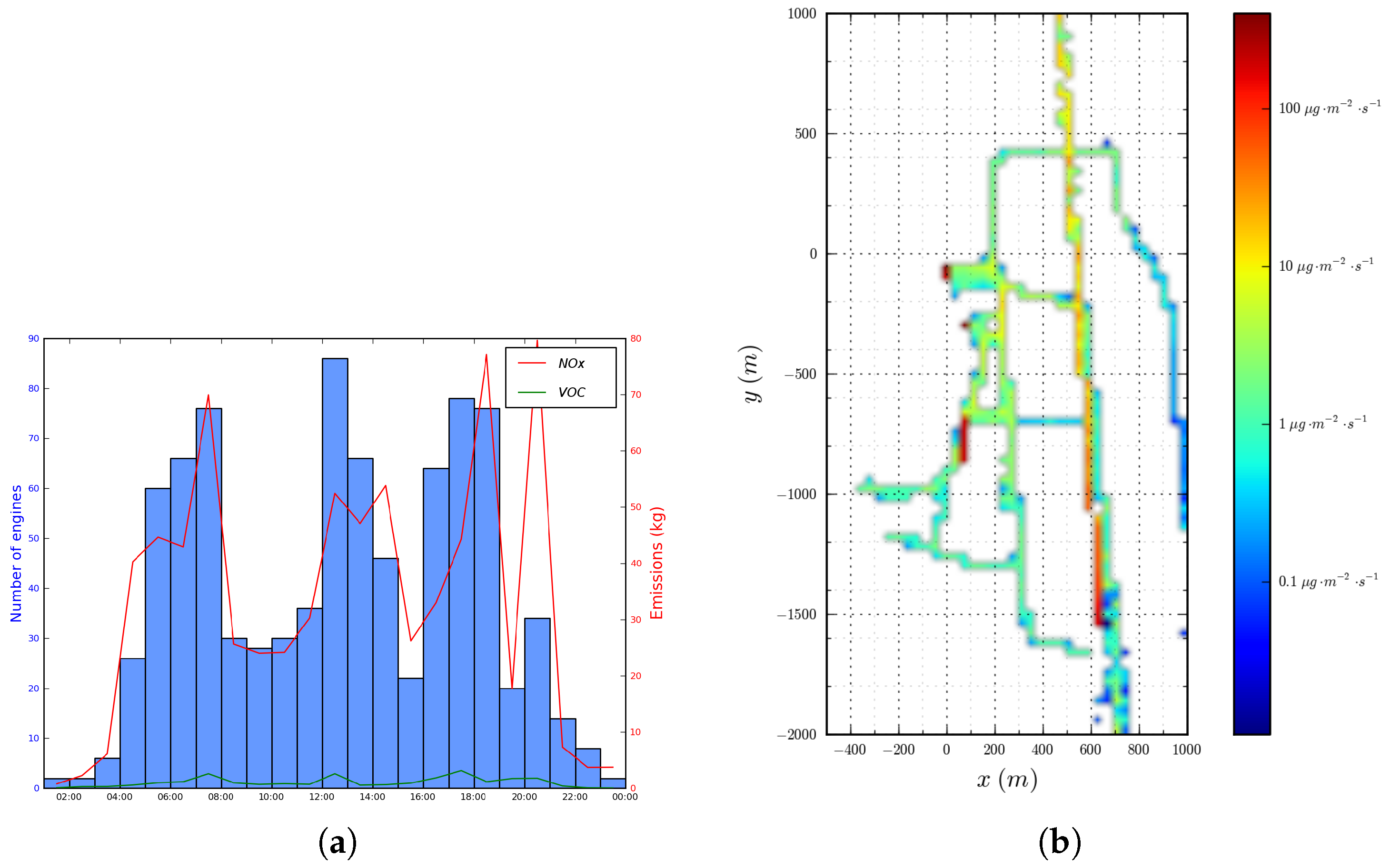
3.1. Building the Emissions Database

In order to compute the emissions database based on real observed data over a regional airport, the aircraft radar streams recorded on 10 September 2010 were analyzed in order to correct and complete the trajectories. These data were provided unofficially and have been kept anonymous.

About 400 aircraft trajectories and 824 engine state vectors were computed from the radar data. Another methodology was applied for a few exceptions such as the piston-engines aircraft, which are not yet implemented in IESTA; some engines used in the traffic are not ICAO-certified or listed in the FOI tables. For that kind of engine, the corresponding trajectories were—for the most part—allocated to equivalent aircraft, or simply ignored if their contribution was deemed negligible.

The emissions of these 824 engines were computed using interpolation in the ICAO tables rather than the IESTA thermodynamic model because of a large variety of engine types. The emissions of NO${}_x$, CO, CO${}_2$, SO${}_2$, and smoke number are computed at a one second time step. As the available data do not include aircraft APU emissions, the ICAO/CAEP Airport Air Quality Manual (ICAO, 2011 [13]) was used to allocate APU emissions to realistic areas and periods. This manual states that an accepted modelling for short-haul aircraft is an APU operating during 45 min and emitting a total of 700 g NO${}_x$, 30 g Unburned HydroCarbons (UHCs), 310 g CO, and 25 g PM10 (particulate matter under 10 $\mathsf{\mu }$m).

As expected, the NO${}_x$ surface emissions were highest near the runway, where the aircraft take off, but also near the parking at the gates as shown in Figure 1, mainly due to APU emissions.

The emissions from sources other than aircraft were provided by a 1 km resolution database at the hourly time step, for the area around the airport. This database has been provided by the local Air Quality Association, in charge of monitoring the air pollution in this region. The NO${}_x$ surface fluxes emitted by aircraft and other anthropogenic sources are injected in the atmospheric model between ground and the first vertical level.

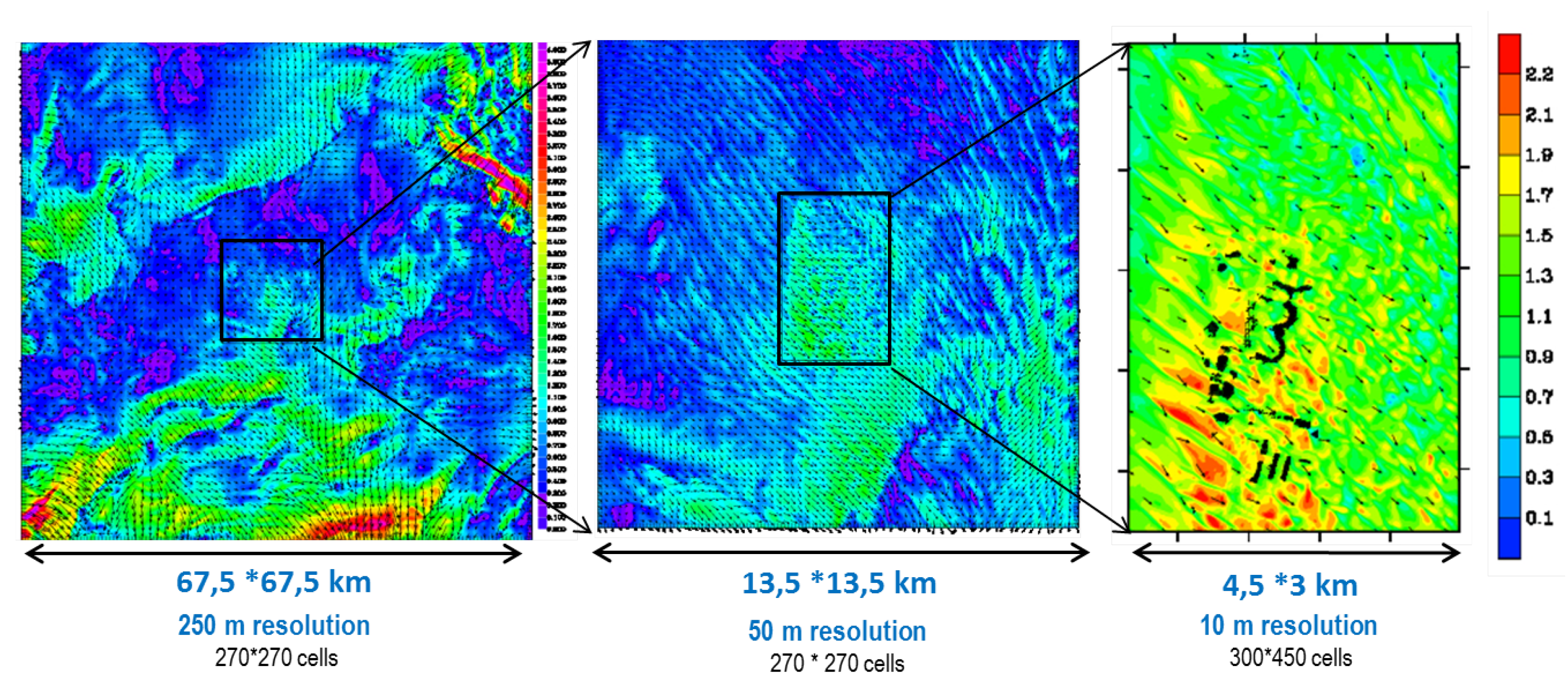
3.2. Initialisation and Land Surface Data

The meteorological situation is initialized using the French Numerical Weather Prediction model AROME analysis (Seity et al., 2010 [26]) at 2.5 km resolution on 10 September 2010 at 6:00 UTC. Analyses are also used for the lateral boundaries forcing every three hours. AROME provides not only initialization and forcing for the dynamical and thermodynamical variables (wind, potential temperature, humidity, etc.) but also surface variables initialization (ground water content, surface temperature, etc.).

In a general context, a spatial resolution of a few tens of metres is necessary to represent most of the eddies of a convective boundary layer. In this case, surface heterogeneities impose a finer resolution and 10 m seems a realistic target.

The grid nesting is also necessary for a downscaling approach from the 2.5 km resolution of AROME. Meso-NH is thus used with three nested domains of simulation, allowing the downscaling from the large-scale forcing model to 250 m resolution for the larger scale domain, 50 m horizontal resolution for the medium one, and 10 m resolution for the smaller one—this latter encompassing only the airport domain (see Figure 2).

Moreover, the fine spatial resolution induces a fine temporal resolution to respect the Courant–Friedrichs–Lewy criterium. The simulation was done with a fourth-order centred scheme to transport the wind, associated to the centred leapfrog scheme. Meteorological and chemical scalars were transported with a PPM (piecewise parabolic method) scheme associated with the forward-in-time stepping scheme. These numerical schemes strongly limit the time step to 1 s at 10 m resolution, but their main interest is their excellent effective resolution (i.e., Ricard et al., 2013 [27]), which is essential to account for the buildings’ impact on the flow and on the pollutant dispersion.

The vertical grid contained 120 levels for the three domains of simulation, with a higher resolution near the ground and stretched above 3000 m. The first level is at 2 m above ground, while 55 levels are included within the first thousand meters.

The land surface parameters are key data for high-resolution modelling of the atmospheric boundary layer (ABL). The surface model, SURFEX, computes surface fluxes for each type of cover according to the characteristics of each tile (albedo, roughness, texture, urbanization, nature, etc.). The land surface covers of the two larger domains were given by the Ecoclimap database derived from the Corinne Land Cover 2000 data (Faroux et al., 2013 [28]).

For the smaller domain, at 10 m resolution and $3\times 4.5$ km width, the surface occupation data came from the OpenStreetMap (OSM) database, which has been converted into the SURFEX surface types. The three main covers as shown on Figure 2c are parking and roads, nature (grassland and crops) and buildings (terminals, train station, hangars) where a drag force is applied according to Aumond et al., 2013 [25] and Bergot et al., 2016 [29].

4. Results

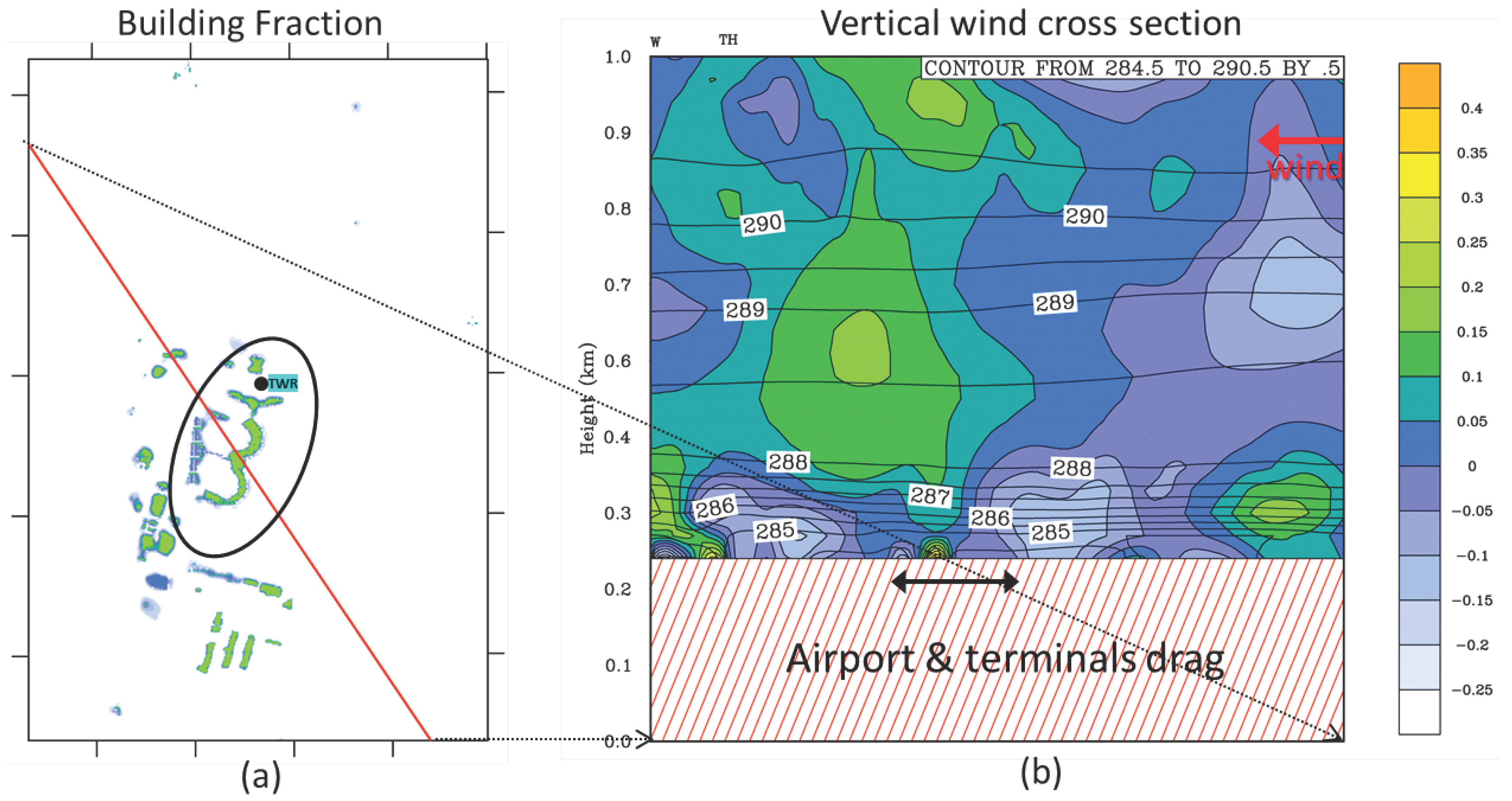
4.1. Dynamic Situation

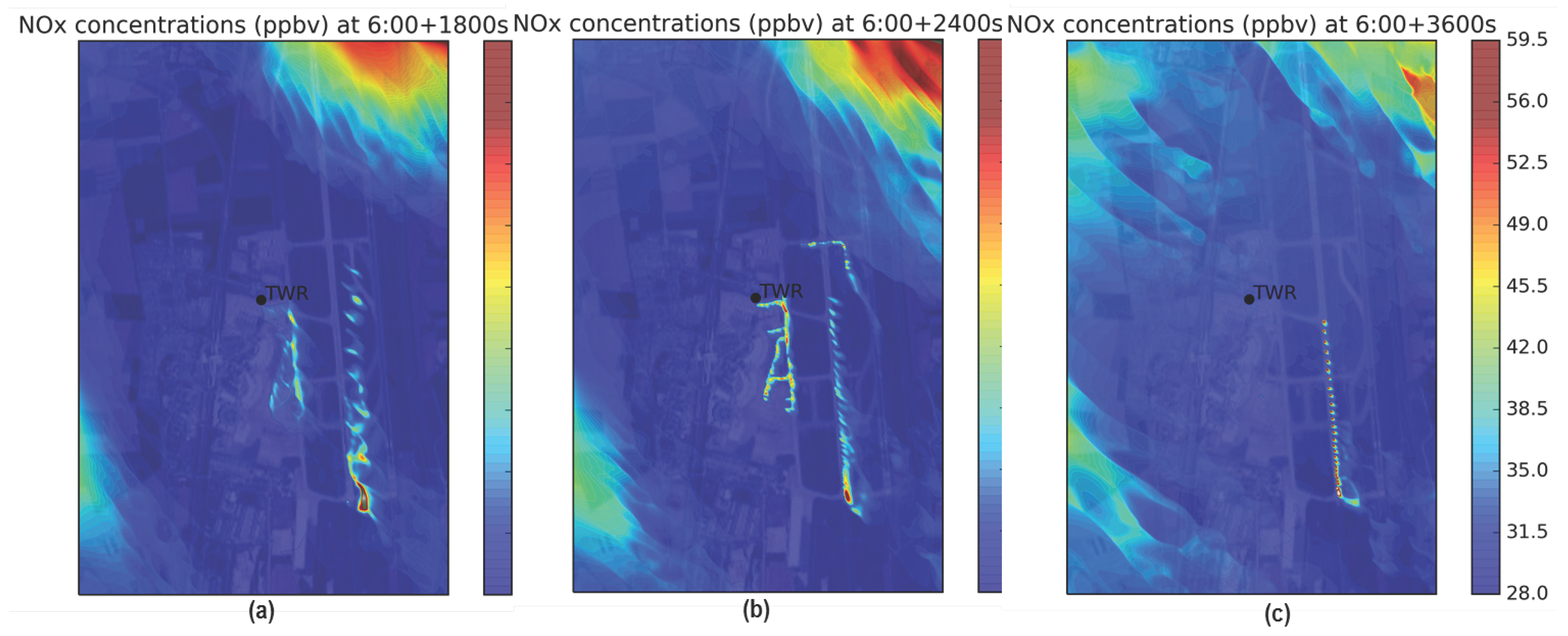
As the morning maximum of aircraft traffic occurs between 6:00 and 8:00 UTC (see Figure 1), the simulation was started at 6:00 UTC on September 10th and ran for 3600 s only, because of a very high CPU consumption.

For this day, the weather conditions were anticyclonic, with high radiation and increasing temperatures. The simulated wind presented low values (less than 2 m/s) over the three domains of simulation (Figure 3), and the direction was from the north-west. During this short period between 6 and 7 UTC, the wind module and direction from Meso-NH were in good agreement with the observations recorded near the control tower (TWR) during the campaign, despite a slight overestimation of the wind module (as shown in Figure 4).

The turbulent kinetic energy (TKE) as well as temperature and wind are impacted by the surface land cover. In fact, the buildings have a strong impact: they increase TKE and temperature, while the vertical wind is positive upstream (due to building obstacles) and negative downstream, thanks to the applied drag force. This phenomenon is shown in Figure 5, which represents a vertical cross-section of the vertical wind component across the airport and between ground and 1000 m. Locally, the vertical wind is positive and enhanced by the presence of the airport terminals. The vertical mixing is consequently enhanced and modified near the buildings, which should noticeably impact the pollutants’ concentrations and dispersion.

4.2. NO_x Dispersion

In this preliminary study, NO and NO${}_2$ are referred to as the total nitrogen oxides (NO${}_x$), and are the only chemical species, introduced in the model as passive scalars. As shown in Figure 6, NO${}_x$ concentrations over the small domain of simulation (10 m resolution) are heterogeneous and higher next to the northern boundary, due to the advection of pollutants from the larger domain and the road traffic emissions. In fact, the wind from north-north-west, albeit low, brings a plume with high level of NO${}_x$. The airport itself seems affected by NO${}_x$ concentration around 50 ppbv; between 6:00 and 6:40 UTC, highs are located right next to the terminals and parkings, where aircrafts’ engines and APUs are operated for longer (Figure 6a). Later, while the air traffic starts to increase, at 7:00, the concentrations are higher along the runway, where aircraft take off.

The NO${}_x$ concentrations are also compared at 6:30 and 7:00 UTC with the TWR observations (Figure 1a). This comparison reveals an underestimation of NO${}_x$ concentration at 7:00 UTC when the NO${}_x$ peak due to the morning traffic is starting. This underestimation is due partly to the dispersive conditions that are too strong in the simulation and to the underestimation of the large-scale northern advection that has not yet reached the airport.

5. Conclusions

A real day of air traffic over a regional airport was simulated using the coupling of two state-of-the-art models: IESTA, modelling the aircraft trajectories and engines emissions, and Meso-NH, for the atmospheric dispersion at 10 m horizontal resolution. In this preliminary study, the NO${}_x$ are considered as passive tracers and the simulation lasts only 3600 s. The coupling of the two models demonstrates the ability to represent not only the aircraft emissions (engines, APU), but also the NO${}_x$ concentration around the terminals’ parking and taxiing areas. Moreover, the meteorological dynamic (low winds and buildings interactions) provides an innovative approach to airport air quality studies at high spatio-temporal resolution. This concept allows better representation of local air quality at airports in order to locate high concentration areas due to the airport specificities (e.g., buildings or power plants), to evaluate the impact of new or future technologies or ATM procedures on the concentration of the main pollutants. This study investigates the feasibility for research purposes, but not for operational forecasting.

The next step for this study is first to continue the simulation all day long in order to determine the evolution of the concentrations in and around the airport. Secondly, the reactive chemistry with photochemistry and ozone–VOC interactions should be added to simulate more realistic behaviour. These improvements are feasible despite needing a large amount of computing time with supercomputers.

References

1. Arunachalam, S.; Wang, B.; Davis, N.; Baek, B.H.; Levy, J.I. Effect of chemistry-transport model scale and resolution on population exposure to PM2.5 from aircraft emissions during landing and takeoff. Atmos. Environ. 2011, 45, 3294–3300. [Google Scholar] [CrossRef]
2. Rissman, J.; Arunachalam, S.; Woody, M.; West, J.J.; BenDor, T.; Binkowski, F. A plume-in-grid approach to characterize air quality impacts of aircraft emissions at the Hartsfield Jackson Atlanta International Airport. Atmos. Chem. Phys. 2013, 13, 9285–9302. [Google Scholar] [CrossRef]
3. Hirtl, M.; Baumann-Stanzer, K. Evaluation of two dispersion models (ADMS-Roads and LASAT) applied to street canyons in Stockholm, London and Berlin. Atmos. Environ. 2007, 41, 5959–5971. [Google Scholar] [CrossRef]
4. Carruthers, D.; Holroyd, R.; Hunt, J.; Weng, W.; Robins, A.; Apsley, D.; Thompson, D.; Smith, F. UK-ADMS: A new approach to modelling dispersion in the earth’s atmospheric boundary layer. J. Wind Eng. Ind. Aerodyn. 1994, 52, 139–153. [Google Scholar] [CrossRef]
5. Peace, H.; Maughan, J.; Owen, B.; Raper, D. Identifying the contribution of different airport related sources to local urban air quality. Environ. Model. Softw. 2006, 21, 532–538. [Google Scholar] [CrossRef]
6. Farias, F.; ApSimon, H. Relative contributions from traffic and aircraft NOx emissions to exposure in West London. Environ. Model. Softw. 2006, 21, 477–485. [Google Scholar] [CrossRef]
7. Holmes, N.; Morawska, L. A review of dispersion modelling and its application to the dispersion of particles: An overview of different dispersion models available. Atmos. Environ. 2006, 40, 5902–5928. [Google Scholar] [CrossRef] [Green Version]
8. Demael, E.; Carissimo, B. Comparative Evaluation of an Eulerian CFD and Gaussian Plume Models Based on Prairie Grass Dispersion Experiment. J. Appl. Meteorol. Climatol. 2008, 47, 888–900. [Google Scholar] [CrossRef]
9. Riddle, A.; Carruthers, D.; Sharpe, A.; McHugh, C.; Stocker, J. Comparisons between FLUENT and ADMS for atmospheric dispersion modelling. Atmos. Environ. 2004, 38, 1029–1038. [Google Scholar] [CrossRef]
10. Aubry, S.; Chaboud, T.; Dupeyrat, M.; Élie, A.; Huynh, N.; Lefebvre, T.; Rivière, T. Evaluating the local environmental impact of air traffic with IESTA: Outputs and validation walkthrough. In Proceedings of the 27th Congress of the International Council of the Aeronautical Sciences, Nice, France, 19–24 September 2010. [Google Scholar]
11. Sarrat, C.; Aubry, S.; Chaboud, T. Modeling air trafic impact on local air quality with IESTA and ADMS-AIRPORT: Validation using field measurements on a regional airport. In Proceedings of the 28th Congress of the International Council of the Aeronautical Sciences, Brisbane, Australia, 23–28 September 2012. [Google Scholar]
12. Schaefer, M.; Bartosch, S. Overview on Fuel Flow Correlation Methods for the Calculation of NOx, CO and HC Emissions and Their Implementation Into Aircraft Performance Software; Technical Report IB-325-11-13; DLR: Cologne, Germany, 2013. [Google Scholar]
13. International Civil Aviation Organization (ICAO). Airport Air Quality Manual. Available online: http://www.icao.int/environmental-protection/Pages/environment-publications.aspx (accessed on 11 April 2017).
14. Swedish Defence Research Agency (FOI). FOI’s Confidential database for Turboprop Engine Emissions. Available online: https://www.foi.se/en/our-knowledge/aeronautics-and-air-combat-simulation/fois-confidential-database-for-turboprop-engine-emissions.htm (accessed on 11 April 2017).
15. Tulet, P.; Crassier, V.; Solmon, F.; Guedalia, D.; Rosset, R. Description of the Mesoscale Nonhydrostatic Chemistry model and application to a transboundary pollution episode between northern France and southern England. J. Geophys. Res. 2003, 108. [Google Scholar] [CrossRef]
16. Sarrat, C.; Lemonsu, A.; Masson, V.; Guedalia, D. Impact of Urban Heat Island on Regional Atmospheric Pollution. Atmos. Environ. 2006, 40, 1743–1758. [Google Scholar] [CrossRef]
17. Sarrat, C.; Noilhan, J.; Dolman, A.; Gerbig, C.; Ahmadov, R.; Tolk, L.; Meesters, A.; Hutjes, R.; Maat, H.T.; Pèrez-Landa, G.; et al. Atmospheric CO2 modeling at the regional scale: An intercomparison of 5 meso-scale atmospheric models. Biogeosciences 2007, 4, 1115–1126. [Google Scholar] [CrossRef]
18. Lac, C.; Donnelly, R.P.; Masson, V.; Pal, S.; Riette, S.; Donier, S.; Queguiner, S.; Tanguy, G.; Ammoura, L.; Xueref-Remy, I. CO2 dispersion modelling over Paris region within the CO2-MEGAPARIS project. Atmos. Chem. Phys. 2013, 13, 4941–4961. [Google Scholar] [CrossRef]
19. Berger, A.; Barbet, C.; Leriche, M.; Deguillaume, L.; Mari, C.; Chaumerliac, N.; Bègue, N.; Tulet, P.; Gazen, D.; Escobar, J. Evaluation of Meso-NH and WRF/CHEM simulated gas and aerosol chemistry over Europe based on hourly observations. Atmos. Res. 2016, 176–177, 43–63. [Google Scholar] [CrossRef] [Green Version]
20. Lafore, J.; Stein, J.; Bougeault, P.; Ducrocq, V.; Duron, J.; Fischer, C.; Héreil, P.; Mascart, P.; Masson, V.; Pinty, J.P.; et al. The Meso-NH atmospheric simulation system. Part I: Adiabatic formulation and control simulations. Ann. Geophys. 1998, 16, 90–109. [Google Scholar] [CrossRef]
21. Cuxart, J.; Bougeault, P.; Redelsperger, J.L. A turbulence scheme allowing for mesoscale and large-eddy simulations. Q. J. R. Meteorol. Soc. 2000, 126, 1–30. [Google Scholar] [CrossRef]
22. Masson, V.; Le Moigne, P.; Martin, E.; Faroux, S.; Alias, A.; Alkama, R.; Belamari, S.; Barbu, A.; Boone, A.; Bouyssel, F.; et al. The SURFEXv7.2 land and ocean surface platform for coupled or offline simulation of earth surface variables and fluxes. Geosci. Model Dev. 2013, 6, 929–960. [Google Scholar] [CrossRef] [Green Version]
23. Noilhan, J.; Planton, S. A simple parametrization of land surface processes for meteorological models. Mon. Weather Rev. 1989, 117, 536–549. [Google Scholar] [CrossRef]
24. Masson, V. A physically based scheme for the urban energy budget in atmospheric models. Bound. Layer Meteorol. 2000, 94, 357–397. [Google Scholar] [CrossRef]
25. Aumond, P.; Masson, V.; Lac, C.; Gauvreau, B.; Dupont, S.; Bérengier, M. Including the drag effects of canopies: Real case large-eddy simulation studies. Bound. Layer Meteorol. 2013, 146, 65–80. [Google Scholar] [CrossRef]
26. Seity, Y.; Brousseau, P.; Malardel, S.; Hello, G.; Bénard, P.; Bouttier, F.; Lac, C.; Masson, V. The AROME-France Convective-Scale Operational Model. Mon. Weather Rev. 2010, 139, 976–991. [Google Scholar] [CrossRef]
27. Ricard, D.; Lac, C.; Riette, S.; Legrand, R.; Mary, A. Kinetic energy spectra characteristics of two convection-permitting limited-area models AROME and Meso-NH. Q. J. R. Meteorol. Soc. 2013, 139, 1327–1341. [Google Scholar] [CrossRef]
28. Faroux, S.; Kaptué Tchuenté, A.T.; Roujean, J.L.; Masson, V.; Martin, E.; Le Moigne, P. ECOCLIMAP-II/Europe: A twofold database of ecosystems and surface parameters at 1 km resolution based on satellite information for use in land surface, meteorological and climate models. Geosci. Model Dev. 2013, 6, 563–582. [Google Scholar] [CrossRef]
29. Bergot, T.; Escobar, J.; Masson, V. Effect of small scale surface heterogeneities and buildings on radiation fog: Large-Eddy Simulation study at Paris-Charles de Gaulle airport. Q. J. R. Meteorol. Soc. 2016, 142, 1029–1040. [Google Scholar] [CrossRef]
Figure 1. (a) NO x and Volatile Organic Compound (VOC) emissions time series with hourly engines aircraft activities; (b) Cumulated surface flux of NO x emissions ( μ g/m 2 /s) on 10 September 2010.
Aerospace 04 00046 g001
Figure 2. Fraction of urban cover on the three domains of simulation interacting in two-ways nesting two ways: (a) 250 m resolution, width = 67.5 km × 67.5 km; (b) 50 m resolution, width = 13.5 km × 13.5 km; (c) 10 m resolution, width = 3 km × 4.5 km.
Aerospace 04 00046 g002
Figure 3. Simulated wind modules and direction over the three domains of simulation 2 m above ground (the first level of simulation), at 7:00 UTC.
Aerospace 04 00046 g003
Figure 4. Observed wind time series (module and direction) and comparisons with the simulation output at 7:00 UTC (orange and blue circles) and observed NO x concentration time series with simulated NO x at 6:30 and 7:00 UTC. TWR: control tower.
Aerospace 04 00046 g004
Figure 5. (a) Surface building fraction (green surfaces represent the airport’s terminal and buildings) and (b) Vertical cross-section of the vertical wind component in m/s for the colored isolines and contours of potential temperature (white labels in K).
Aerospace 04 00046 g005
Figure 6. NO x concentration (ppbv) at 2 m above ground: (a) at 6:30 UTC; (b) at 6:40 UTC; (c) at 7:00 UTC.
Aerospace 04 00046 g006