Article

Guidance, Navigation and Control of Unmanned Airships under Time-Varying Wind for Extended Surveillance

Department of Mechanical and Aerospace Engineering, University of Texas at Arlington, 211 Woolf Hall, Box 19018, 500 W. First St., Arlington, TX 76010, USA
*
Author to whom correspondence should be addressed.
Aerospace 2016, 3(1), 8; https://doi.org/10.3390/aerospace3010008
Submission received: 21 December 2015 / Revised: 20 January 2016 / Accepted: 10 February 2016 / Published: 17 February 2016
(This article belongs to the Collection Unmanned Aerial Systems)

Abstract

:
This paper deals with the control of lighter-than-air vehicles, more specifically the design of an integrated guidance, navigation and control (GNC) scheme that is capable of navigating an airship through a series of constant-altitude, planar waypoints. Two guidance schemes are introduced, a track-specific guidance law and a proportional navigation guidance law, that provide the required signals to the corresponding controllers based on the airship position relative to a target waypoint. A novel implementation of the extended Kalman filter, namely the scheduled extended Kalman filter, estimates the required states and wind speed to enhance the performance of the track-specific guidance law in the presence of time-varying wind. The performance of the GNC system is tested using a high fidelity nonlinear dynamic simulation for a variety of flying conditions. Representative results illustrate the performance of the integrated system for chosen flight conditions.

Graphical Abstract

1. Introduction

The dream of controlled flight was first realized by the invention of the airship, where it is claimed that Jean-Baptiste Meusnier designed the first airship in 1748 [1]; it however, lacked a lightweight, powerful engine. Henri Giffard was the first person to equip an airship with steam-engine technology successfully. He flew his airship 17 miles in 1852, with a single propeller driven by a three-horsepower engine [2]. The airship’s golden age was launched by the German Luftschiff Zeppelin in 1900, which was utilized in commercial and military applications. That golden age tragically ended in the Hindenburg disaster in 1937. In the past couple of decades, however, interest in airships arose due to the advancement of technology in many engineering fields. New demands, which cannot be satisfied by conventional fixed-wing aircraft, have also enthused interest in airships [3]. Therefore, analyzing the dynamics of airships and implementing control structures that guarantee high performance and safety are necessary for the continued advancement of aerospace technology.
An airship’s main source of lift is buoyancy, or static lift. This is based on Archimedes’ principle: if a body is immersed in a fluid (air), it experiences a force proportional to the volume of the displaced fluid in the opposite direction of its weight. When the density of the body (airship) is less than that of the fluid (air), that force is substantial. Due to this, the dynamics of an airship are different from that of a conventional aircraft, with significant effects from added mass and added inertia and a much higher sensitivity to wind [4]. Added mass and inertia effects are changes in the dynamics of the airship due to the mass and inertia of the air in which it is flying. This is experienced by all aircraft; however, in heavier-than-air flight, the mass and inertia of air are negligible when compared to that of the aircraft. In lighter-than-air flight, however, such as airship flight, these effects have too profound of an effect on the dynamics that they cannot be neglected. Due to this method of operation, airships have the ability to hover. This ability can transform unmanned airships into data acquisition platforms ideal for applications, such as surveillance, terrain mapping, climate research, inspection of man-made structures and GPS [5].
The ability to stabilize and control an airship under wind disturbances is vital in any application. PID control is a commonly-used control scheme in various applications; the AURORA airship project, focused on the development of sensing, control and navigation technologies for autonomous or semi-autonomous airships [6], employs a PID controller for the longitudinal velocity control, a PD altitude controller and a PD controller for heading control. A different approach, developed to control the airship heading, incorporates a PID controller with gains designed using H 2 / H methods [7]. Neural network-augmented model inversion control is also applied to airship control [8]; it is a combination of feedback linearization and linear control. The theoretical aspect of applying the neural network is to compensate for the feedback linearization and modeling error. A dynamic inversion control law, forcing the closed-loop system outputs to follow a position command trajectory, is also designed to give an airship path-tracking capability [9]. The control law shows fast correction of trajectory errors. Lyapunov stability-based designs of state-feedback control laws have also been implemented for the airship control problem [10]. A backstepping methodology is utilized to design a closed-loop trajectory-tracking controller for an under-actuated airship [11]. The authors state that backstepping is suitable for the cascaded nature of the vehicle dynamics and that it offers design flexibility and robustness against parametric uncertainties, which are often encountered in aerodynamic modeling and air stream disturbances. Other methods, including sliding mode control [12], and fuzzy logic design, are implemented for airship control [13].
The work presented here focuses on the design of a sub-optimal gain-scheduled feedback control law based on linear quadratic (LQ) methods. This controller is expected to fly the airship through a series of planar waypoints based on commands generated by a track-specific navigation algorithm. The selection of an LQ-based controller design is accredited to its ability to deal with multi-variable systems in a relatively simple way and its ease of implementation [14]. While the presented work is similar to [15] and [16], who implement an LQ controller for regulating airship navigated flight, neither the exact gain scheduling law nor the navigation law used to guide the airship through flight are discussed in detail. In [16], eleven trim points are required to implement a gain scheduling law, and the guidance law generates a commanded yaw rate based on the airship heading and the commanded heading towards the next waypoint. The work presented here introduces a simplistic, yet highly effective gain scheduling law with the capability of supplying the controllers with the values of the gain during all flight modes and relies on fewer trim points for achieving similar tasks.
The paper also presents two guidance laws; the first is a path-specific guidance law, commanding the airship to visit planar waypoints along a specified path. The other is a proportional navigation guidance law, commanding it to visit the waypoints by rotating its velocity vector. Both [15] and [16] assume that the required states and state derivatives to implement the control and navigation laws are available. This is not always true in reality, where some states may not be available by measurement. This issue is addressed in the work presented in this paper by designing and implementing a novel scheduled extended Kalman filter (SEKF) to estimate the required states for control and navigation with a minimal sensor suite on-board the airship. Measurements are only available from an inertial measurement unit (IMU) and GPS sensors. The EKF is presented in a manner such that the nonlinear system dynamics’ Jacobians need not be calculated at every instant, but are precalculated for a set of flight modes, and a “Jacobian scheduling law” is utilized to supply the filter with the needed values at every instant of the flight. This approach is not computationally intense and does not require the formulation of expressions for the Jacobian entries; therefore, it is effective and time saving. The governing equations of motion for the airship are complex; thus, having numerically-precalculated Jacobian matrices for every flight segment and scheduling these values allow for a practically effective approach for applying an EKF algorithm.
The paper is organized as follows: the airship nonlinear equations of motion are introduced first followed by the required linear models for control design, which are presented and discussed. The control laws and their corresponding navigation laws are designed and discussed. Following this, a novel EKF implementation for state and parameter estimation is elucidated. Finally, the results obtained from this research are introduced and discussed to formulate a conclusive argument.

2. Equations of Motion

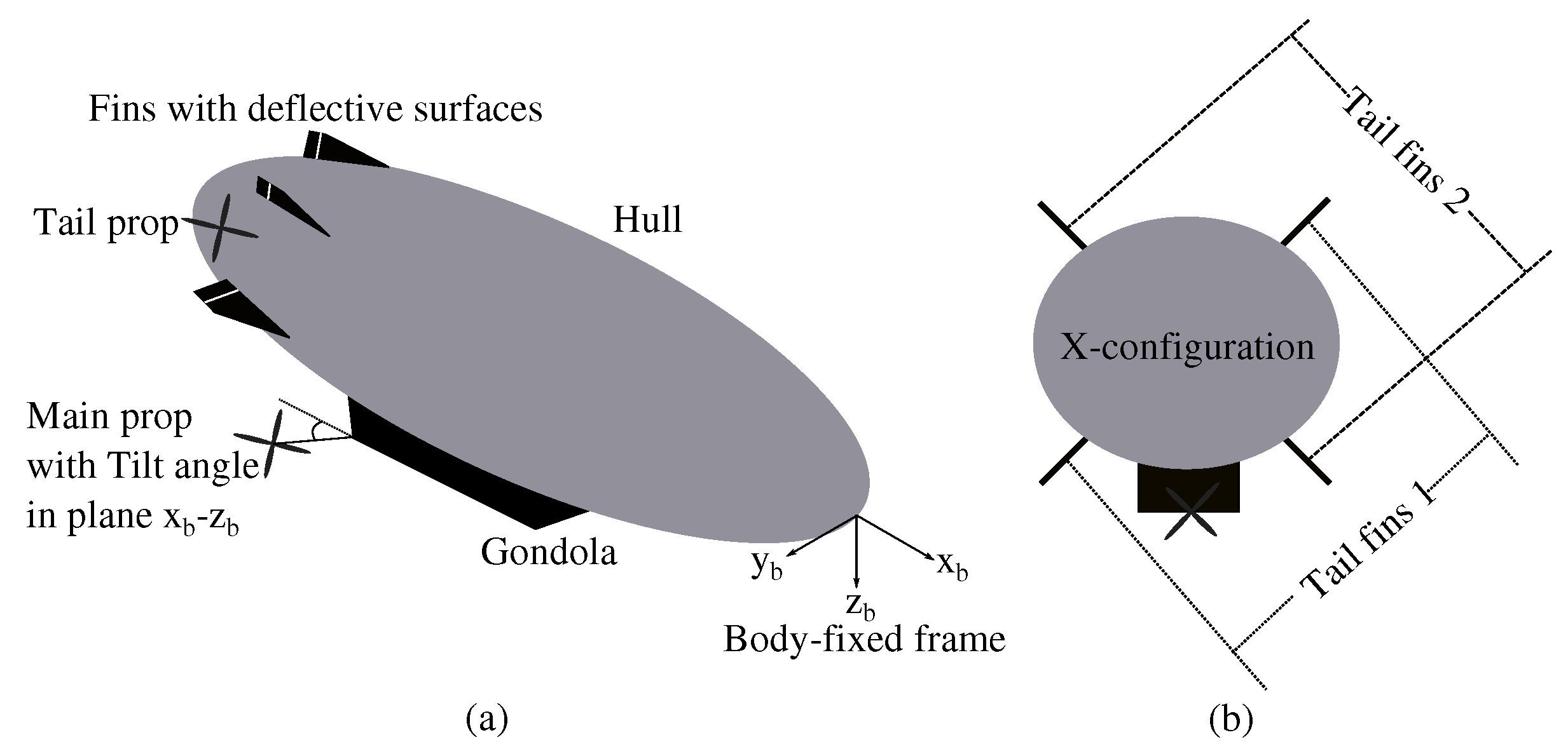
The unmanned airship selected for this work is the AS500 airship [17,18,19,20]. The AS500 has a main hull engulfing the lifting gas, as can be seen in Figure 1a. The AS500 incorporates aerodynamic tail fins in an X -configuration; these fins include control surfaces that can be deflected for stability and control. The tail fin configuration can be seen in Figure 1b, where it is clear that there are two groups of fins: Groups 1 and 2. The X -configuration implies that the control of the airship flight is achieved by a coordinated effort between both fin group deflections Δ 1 and Δ 2 .
The AS500 main propeller, with tilting capability in the x z plane of the body-fixed frame at an angle γ T m , is positioned below the hull along the gondola, which is illustrated in Figure 1a. A tail propeller that aids in heading control is also available on the AS500 and is illustrated in the figure. Numerical values for some of the airship physical parameters are given in Table 1.
The equations of motion presented here are based on the methodology presented in [19,20,21]. The derivation is omitted here for brevity; however, a detailed one can be found in [22]. The airship motion in the inertial frame is the sum of the airship motion relative to the atmosphere and the atmosphere’s inertial motion. Therefore, the translational kinematics of the airship can be described as:
r ˙ a = R I B T V + W
where R I B is the rotation matrix from the inertial frame to the body frame, r a is the position vector of the airship’s body frame origin, expressed in the inertial frame, r a = [ x y z ] T , V is the vector of airship velocity relative to the atmosphere expressed in the body frame, V = [ u v w ] T , and W is the atmosphere inertial velocity vector expressed in the inertial frame, W = [ W x W y W z ] T 
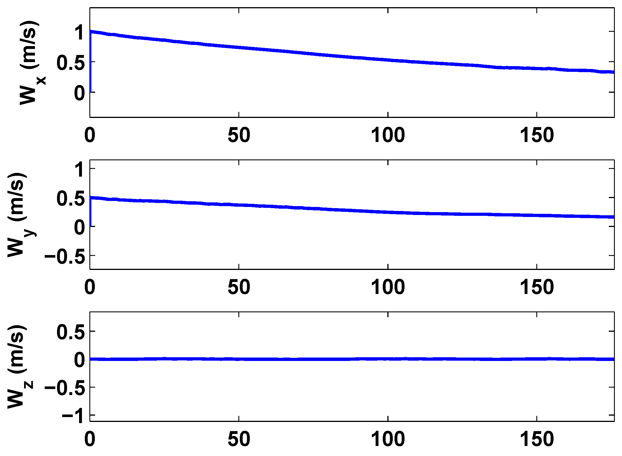
. The prevailing wind field experienced by the airship is simulated using the exponentially correlated wind model (ECWM) [23]. The equations that govern the change of wind speed, in the inertial frame, are:
W ˙ x = b w W x + a w b w η x W ˙ y = b w W y + a w b w η y W ˙ z = 0 W ¨ x = 0 W ¨ y = 0 W ¨ z = 0
with a w as a coefficient showing the extent of the mean square value of the wind, b w the inverse time constant to show the extent of the correlation of the wind and η x and η y being the zero-mean Gaussian white noise. a w and b w are calculated as a w = 2 ( E { W } 2 + σ 2 w ) and b w = 1 τ w . Wind parameter values are summarized in Table 2. The wind is assumed to have a zero-mean Gaussian distribution, with a standard deviation of 0.5 m/s. The Dryden model is utilized to add the turbulence effect to the wind model.
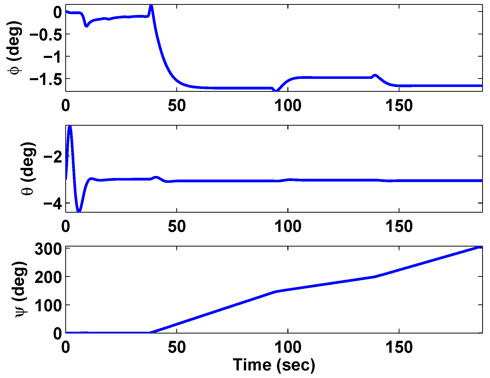
The rotation matrix from the inertial frame to the body frame is constructed based on the 3-2-1 Euler angle rotation sequence. The rotational kinematics expresses the mapping of the body angular velocity to the Euler angle rates.
Ω ˙ = Γ ( Ω ) ω B I
where Ω = [ ϕ θ ψ ] T , with φ, θ and ψ being the roll, pitch and yaw angles. Γ(Ω) is shown below.
Γ ( Ω ) = 1 sin ( ϕ ) tan ( ϕ ) cos ( ϕ ) tan ( ϕ ) 0 cos ( ϕ ) sin ( ϕ ) 0 sin ( ϕ ) sec ( θ ) cos ( ϕ ) sec ( θ )
The governing equations of motion for the airship translational and rotational dynamics, respectively, are:
V ˙ = ( M I 3 × 3 ) 1 ( F 0 + F 1 V ˙ + F 2 ω ˙ B I F A + T m + T t + F b g B ) + [ ω B I ] × V R I B W ˙ [ ρ c m ] × ω ˙ B I [ ω B I ] × 2 ρ c m
ω ˙ B I = I M 1 ( M 0 + M 1 ω ˙ B I + M 2 V ˙ M A + M p + M b o u y + M g + M [ ρ c m ] × ( [ ω B I ] × V + V ˙ + R I B W ˙ ) + [ ω B I ] × I M ω B I )
where M is the scalar mass of the airship, ρ c m is the center of mass position vector relative to the body frame, expressed in the body frame, I 3 × 3 is an identity matrix, I M is the inertia tensor and ω B I is the airship angular velocity vector with respect to the inertial frame expressed in the body frame as ω B I = [ p q r ] T (the roll, pitch and yaw rates). F 0 , F 1 , F 2 , T m , T t , F b g B , M 0 , M 1 , M 2 , M p , M b o u y and M g are variables pertaining to the forces and moments acting on the airship and are to be discussed next.

Forces and Moments on the Airship

The aerodynamic model implemented here is based on published data [20]. The aerodynamic forces acting on the airship during flight are expressed as:
F A = F 0 + F 1 V ˙ + F 2 ω ˙ B I
where F 1 and F 2 are the virtual mass matrices, whose expressions are given in Appendix B (see Equations (23) and (24)). F 0 is the main aerodynamic force vector in the body frame and can be expressed as:
F 0 = F x B F y B F z B = 1 2 ρ a i r | | V | | 2 S r e f C T 1 2 ρ a i r | | V | | 2 S r e f C L 1 2 ρ a i r | | V | | 2 S r e f C N D u V ω B I
C T , C L , C N are aerodynamic force coefficients in the body frame X-direction, Y-direction and Z-direction, respectively, and the expressions for these coefficients are given in Appendix A. S r e f is the reference surface area of the airship hull; D u is the translational section of the Coriolis-centrifugal coupling matrix; and ρ is the air density. Appendix B shows the expression for the the Coriolis-centrifugal coupling matrix. The aerodynamics moments acting on the airship during flight can be expressed as:
M A = M 0 + M 1 ω ˙ B I + M 2 V ˙
where M 1 and M 2 are the virtual inertia matrices, whose expressions are given in Appendix B (see Equations (25) and (26)). M 0 is the main aerodynamic moment vector in the body frame and can be expressed as:
M 0 = M x B M y B M z B = 1 2 ρ a i r | | V | | 2 S r e f L r e f C l 1 2 ρ a i r | | V | | 2 S r e f L r e f C m 1 2 ρ a i r | | V | | 2 S r e f L r e f C n D ω V ω B I
C l , C m , C n are the aerodynamic moment coefficients in the body frame X-direction, Y-direction and Z-direction respectively. Expressions for the aerodynamic moment coefficients are given in Appendix A, as well. L r e f is the reference length of the airship hull, and D ω is the rotational section of the Coriolis-centrifugal coupling matrix (see Appendix B).
The AS500 airship has two sources of thrust, the main propeller and the tail propeller. The main propeller can produce thrust in the body frame X- and Z-directions by rotating at an angle γ T m . The tail propeller only produces thrust in the y-direction of the body frame. The two vectors can be expressed in the body frame as T m = [ T m cos ( γ T m ) 0 T m sin ( γ T m ) ] T and T t = [ 0 T t 0 ] T , where T m and T t are the magnitude of the main and tail thrust, respectively. The moment due to the propulsive forces acting on the airship in the body frame can be expressed as the sum of the cross product of the force vectors and their locations as M p = ρ T m × T m + ρ T t × T t , where ρ T m and ρ T t are the position vectors of the main and tail propeller, respectively, in the body frame. The buoyancy and weight are both represented in the inertial frame as one buoyancy-weight vector F b g I = [ 0 0 ( F g F b ) ] T ; therefore, to express the buoyancy-weight force vector in the body frame, it is pre-multiplied by the rotation matrix as follows F b g B = R I B F b g I , and the moment due to the buoyancy force can be expressed as M b o u y = ρ c v × R I B F b I , where ρ c v is the location of the center of volume in the body frame, expressed in the body frame, and F b I is the buoyancy force acting on the airship expressed in the inertial frame. The moment due to the weight can be expressed as the product of the location of the center of mass and the weight vector in the body frame M g = ρ c m × R I B F g I , where F g I is the weight of the airship expressed in the inertial frame.
  • γ T m Main propeller tilt angle
  • T m Main propeller thrust vector
  • ρ T m Main propeller position vector
  • T t Tail propeller thrust vector
  • ρ T t Tail propeller position vector
  • M p Moment due to the propulsive forces
  • F b g I Buoyancy-weight vector in the inertial frame, expressed in the inertial frame
  • F b g B Buoyancy-weight vector in the inertial frame, expressed in the body frame
  • M b o u y Moment acting on airship due to buoyancy force
  • M g Moment acting on airship due to gravitational force
  • ρ c v Location of the center of volume in the body frame, expressed in the body frame
  • ρ c m Location of the center of mass in the body frame, expressed in the body frame
The defined forces and moments acting on the airship combined with the nonlinear equations of motions presented earlier can be used to generate a nonlinear simulation of the airship flight.

3. Trim Conditions and the Linear Model

The airship nonlinear model discussed earlier is trimmed at two flight conditions; straight and level flight and level turn flight. The airship speed is held constant during flight. The airship will visit planar waypoints pre-programmed into the guidance algorithm in the order they are given, while maintaining constant altitude. The AS500 airship is capable of speeds up to 12.5 m/s [17]; therefore, it is assumed that it can operate safely at a trim speed of 7 m/s. A trim altitude of 1000 m can be achieved if the correct mass of helium is loaded into the hull of the AS500. Since the volume of the AS500 is 15 m3, it is assumed that the helium in the hull will expand to that volume at the trim altitude, but no more to prevent any damage. To do so, the mass of the helium loaded into the airship at sea level must account for such expansion; the following calculations show how this is possible.
The volume of the airship at sea level and the volume at 1000 m are related as follows [4], V 0 = σ V 1000 , where σ is the ratio of air density at 1000 m, and the air density at sea level is approximately 0.9. Setting V 1000 equal to 15 m3 gives V 0 = 13.5 m3. The volume at sea level is related to the mass of helium by V 0 = M H e / ρ H 0 , where M H e and ρ H 0 are the mass of helium and the density of helium at sea level, respectively. This calculation results in a required mass of 2.4 kg of helium to be loaded into the airship’s hull. The value of the states and inputs at each trim point are given in Table 3; where T M , γ T M , T t , Δ 1 and Δ 2 are the main rotor thrust, main rotor tilt angle, the stern rotor thrust and the deflections of the aerodynamic control surfaces, respectively.
  • σ Air density ratio
  • M H e Mass of helium
  • ρ H 0 Density of helium at sea level
  • Δ 1 Deflection of control surface on tail fin Group 1
  • Δ 2 Deflection of control surface on tail fin Group 2
To employ linear quadratic methods for obtaining the optimal gains for controlling the airship, a linear state-space model of the airship dynamics is required. Note, the wind terms are set to zero for trim analysis. The nonlinear model formed by Equations (1), (3)–(5) can be linearized about the two trim points in Table 3, and the two linear state-space models having the form below are achieved:
δ X ˙ = A δ X + B δ U
where A is the system matrix, B is the input matrix and δ U and δ X are the incremental input and state vectors, respectively, and can be represented as follows:
δ X = [ δ u δ v δ w δ p δ q δ r δ x δ y δ z δ ϕ δ θ δ ψ ] T δ U = [ δ T M δ γ T M δ T t δ Δ 1 δ Δ 2 ] T
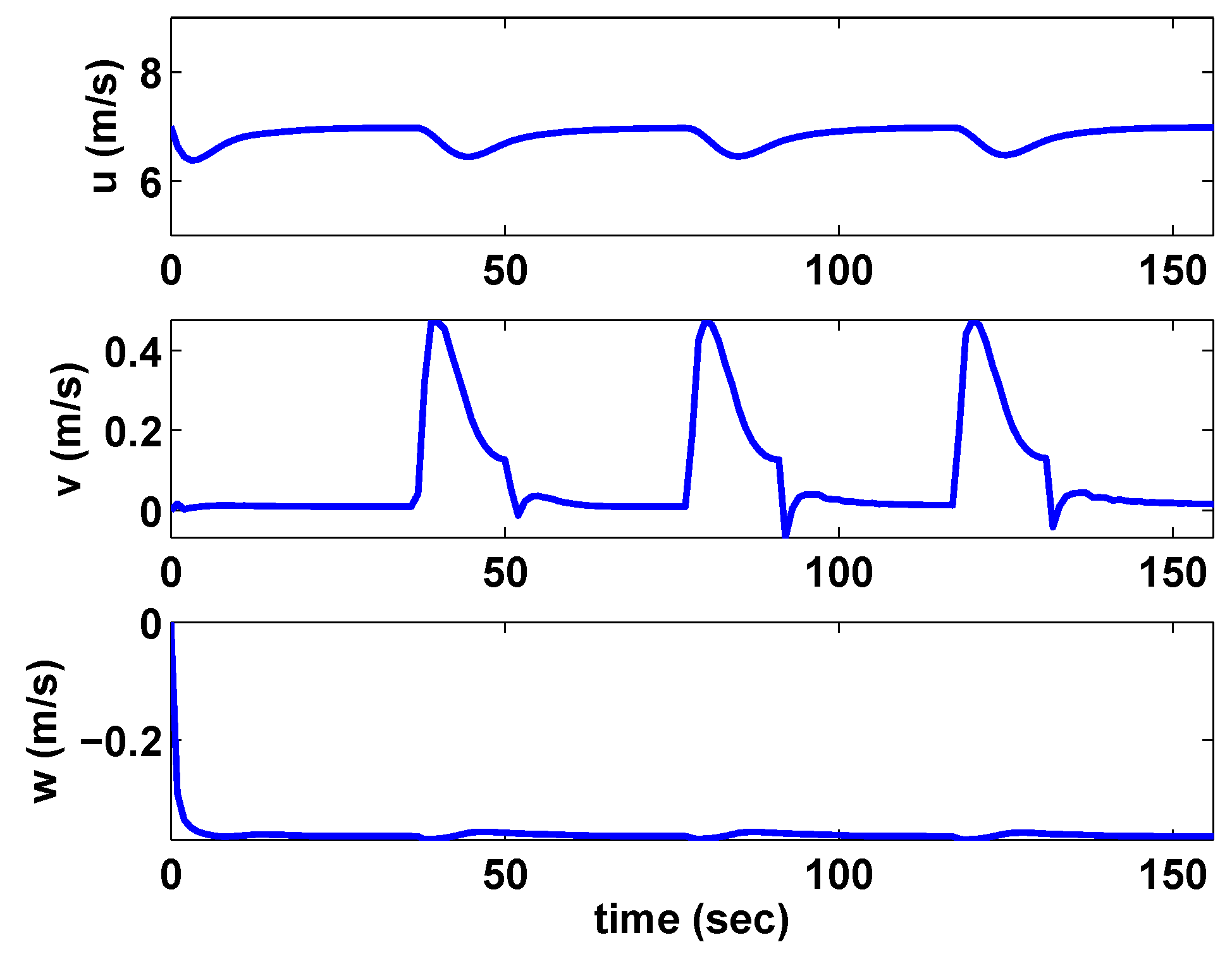
  • u Speed along the body x-direction
  • v Speed along the body y-direction
  • w Speed along the body z-direction
  • p Rotation rate along the body x-direction
  • q Rotation rate along the body y-direction
  • r Rotation rate along the body z-direction
  • x Position in the inertial x-direction
  • y Position in the inertial y-direction
  • z Position in the inertial z-direction

4. Linear Quadratic (LQ) Control and Guidance Laws

The linear-quadratic optimal control problem is an optimization problem that finds a state-feedback control law of the form δ U = K δ X , which minimizes a quadratic performance index subject to a linear dynamical constraint in Equation (10) [14]. The performance index is of the following form:
J = 0 ( δ X T Q δ X + δ U T R δ U ) d t
where Q is an n × n weighting matrix and is typically positive-semidefinite and n is the number of states, which in our case is equal to 12. R is an m × m positive-definite weighting matrix, where m is the number of inputs and is equal to five for the AS500 airship model. Suitable values for Q and R are selected based on the approaches highlighted in [24,25,26,27]. More specifically, we employ the method of [27] for this work. The control gains are obtained by using the solution of the algebraic Riccati equation,
A T P + P A + Q P B R 1 B T P = 0
and, thus, K = R 1 B T P . To enable set point tracking, the control law is implemented as, U = K ( X X t r i m ) + U t r i m , where X is the state vector, X t r i m is the value of the trim states at the current flight condition, U t r i m are the trim values for the inputs at the same flight condition and K is the same gain matrix calculated earlier.

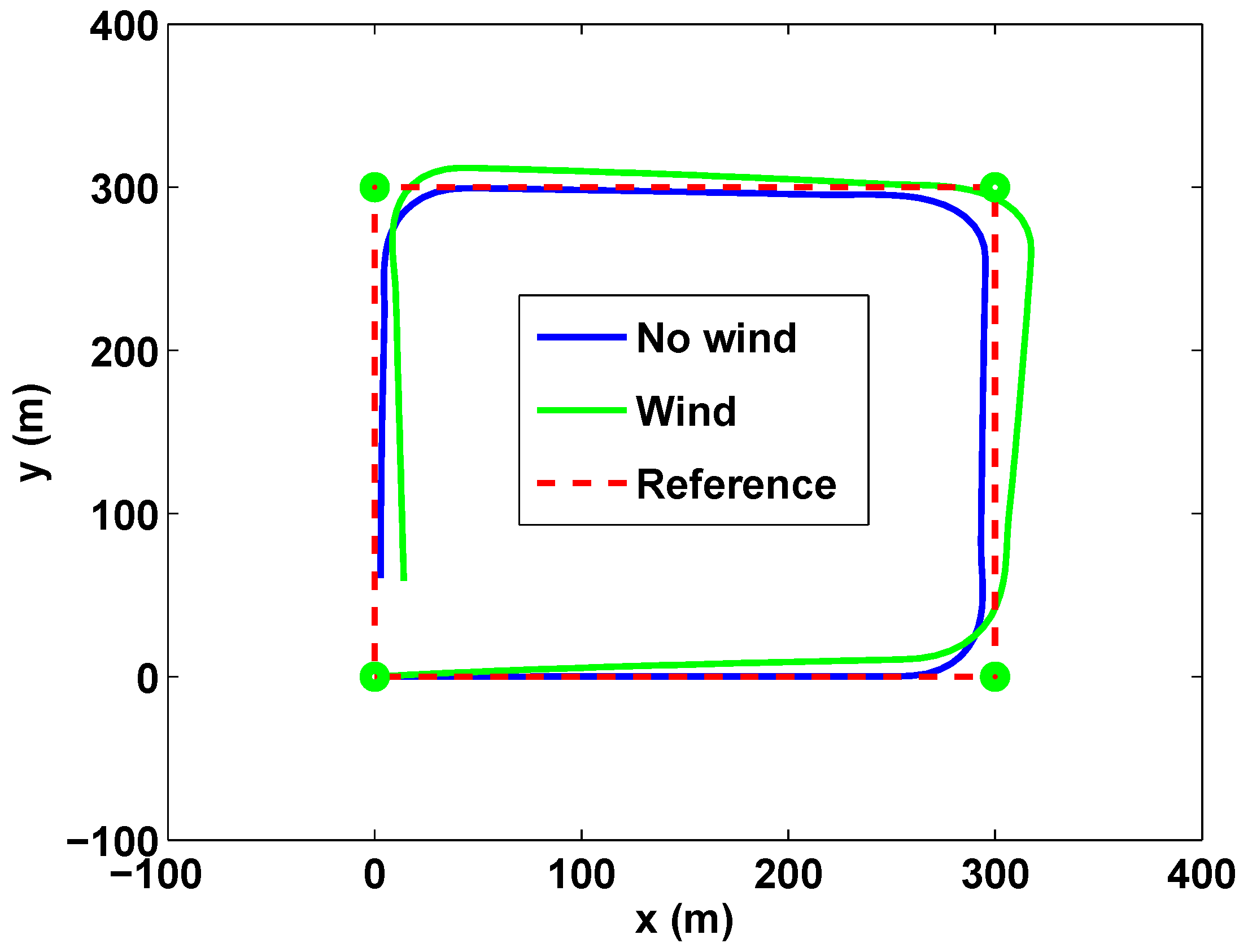
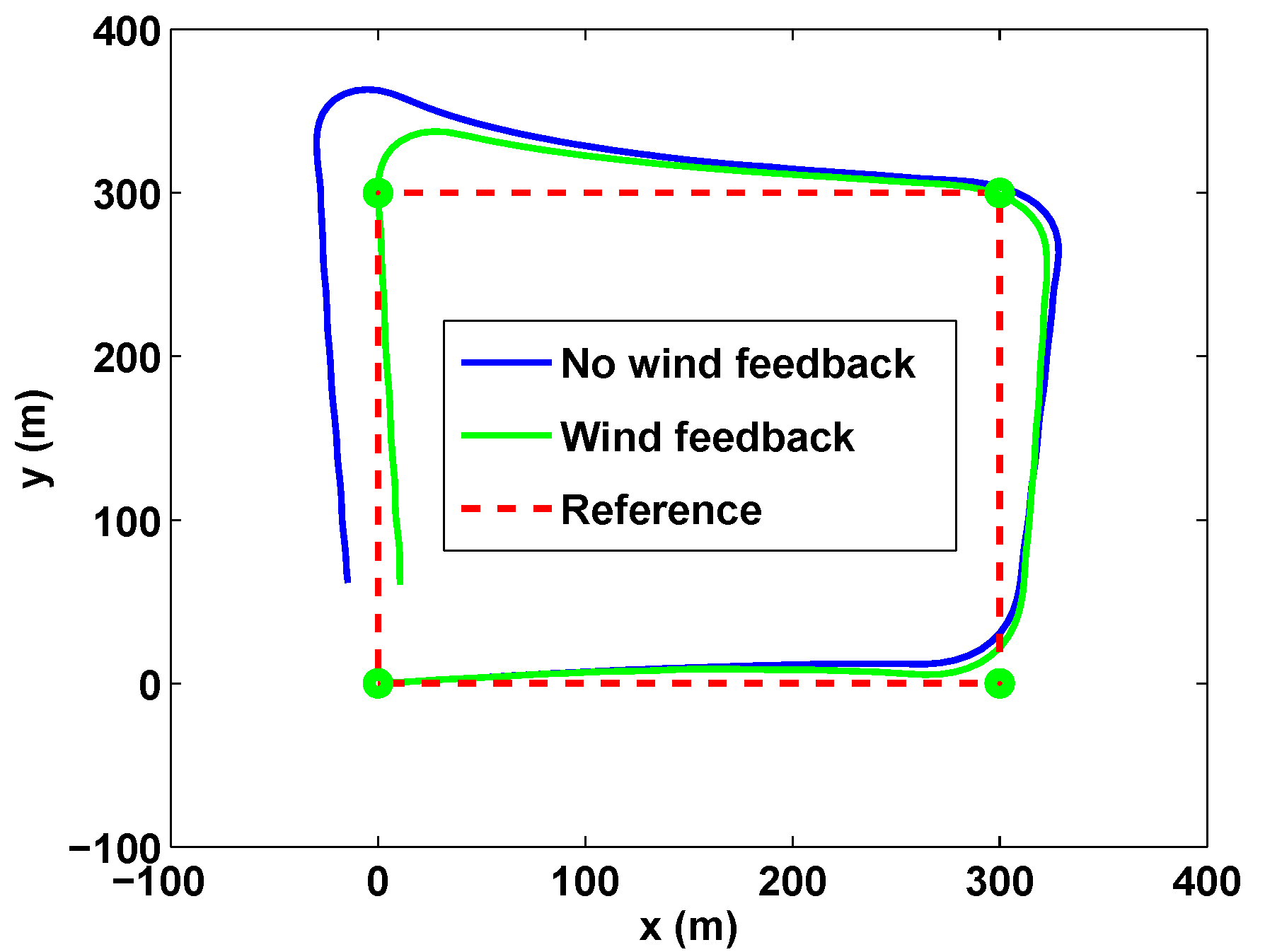
4.1. Track-Specific Guidance Law

A reference signal must be supplied to the controller, in order for it to make the required adjustments to the inputs and fly the airship in a stable manner towards the next waypoint. This reference signal, in the work presented here, is based on a required airship heading and its location relative to the next waypoint. The airship must navigate through a set of constant-altitude, planar waypoints; therefore, a track-specific guidance law is developed below. Note, nonlinear path following strategies using Lyapunov techniques for mini air vehicles are also discussed in [28]. Additionally, trajectory generation for tracking is discussed in [29], wherein Dubin’s model is used. While Dubin’s model is very helpful in generating smooth planar trajectories, we consider the full nonlinear model where the altitude and speed of the vehicle change as it goes through the waypoints. In the present paper, reference paths (trajectories) are not generated; only the waypoints are utilized to generate heading commands.
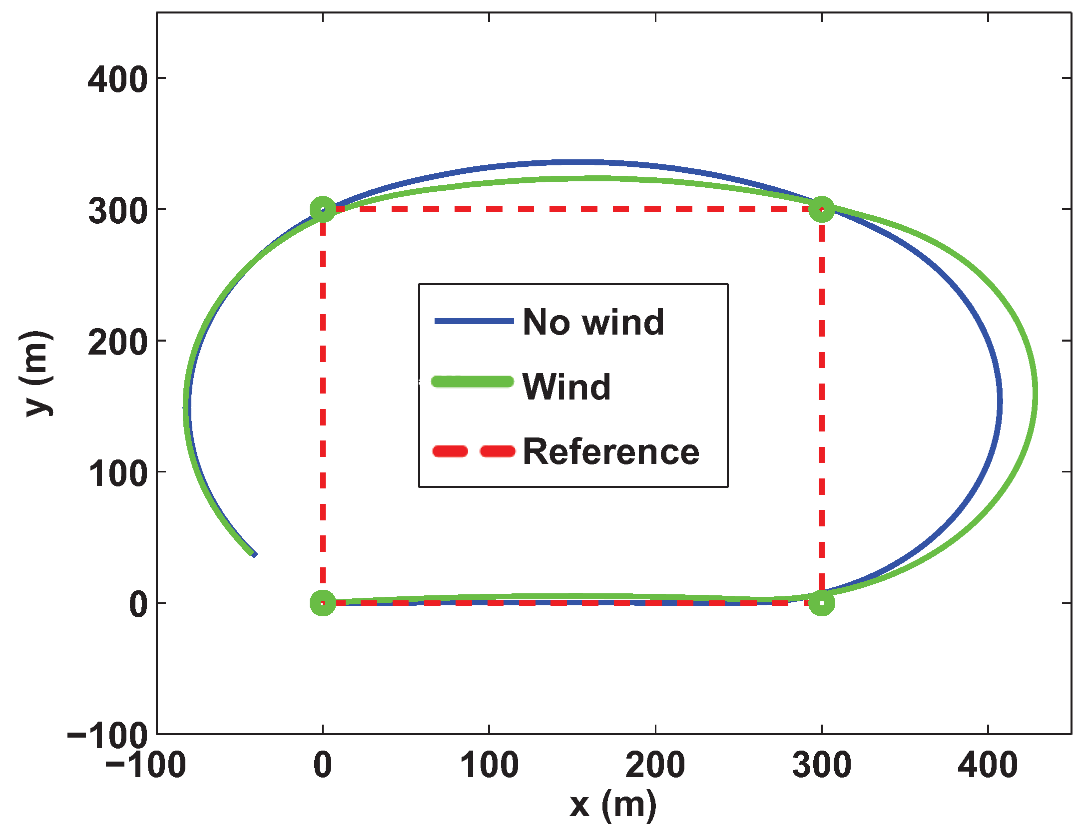
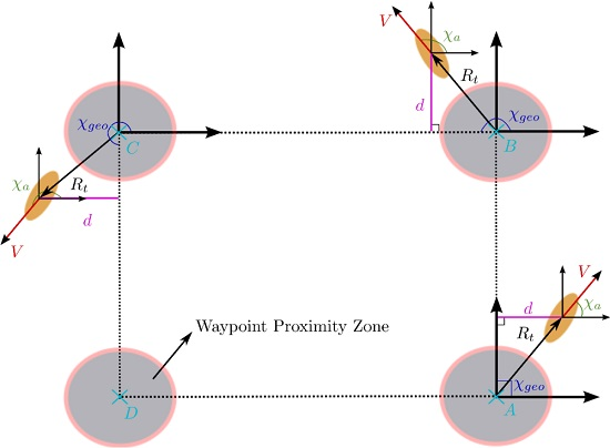
If the airship were to visit four waypoints, A , B , C and D, in that order, the guidance law will track the waypoints in pairs, such that when the airship is flying from A to B, the track-specific (TS) guidance law will track both the A and B locations. A geometric heading based on the location of this pair of waypoints is calculated using A x , A y , B x and B y , which are the x and y coordinates of waypoints A and B, respectively. Thus, χ g e o = tan 1 B y A y B x A x .
The heading of the airship is calculated based on its projected ground speed as χ a = tan 1 y ˙ x ˙ . Using the geometric and airship heading values, a desired heading angle is calculated, i.e., χ d = π 2 tanh d L d e s , where d is the normal distance to the virtual straight line path connecting the waypoints, shown in Figure 2, and is obtained as d = R t sin χ g e o χ a , where R t is the distance traveled from waypoint A and L d e s is a design parameter, which is a function of the airship speed and calculated as, L d e s = V τ , with τ being a performance design parameter.
  • χ g e o Geometric heading
  • χ a Airship heading
  • χ d Airship desired heading
  • ψ c o m m Commanded yaw angle
The commanded yaw angle provided to the set-point tracking controller is calculated as ψ c o m m = χ d β , where β is the airship side-slip angle.
A virtual waypoint proximity zone, with a predefined radius, surrounds each waypoint. As the airship flies towards a waypoint, it will do so in a straight and level flight manner. When the proximity zone is breached, the tracked waypoint set changes by looking ahead towards the next waypoint, and so on. The track-specific guidance law methodology is illustrated in Figure 2.

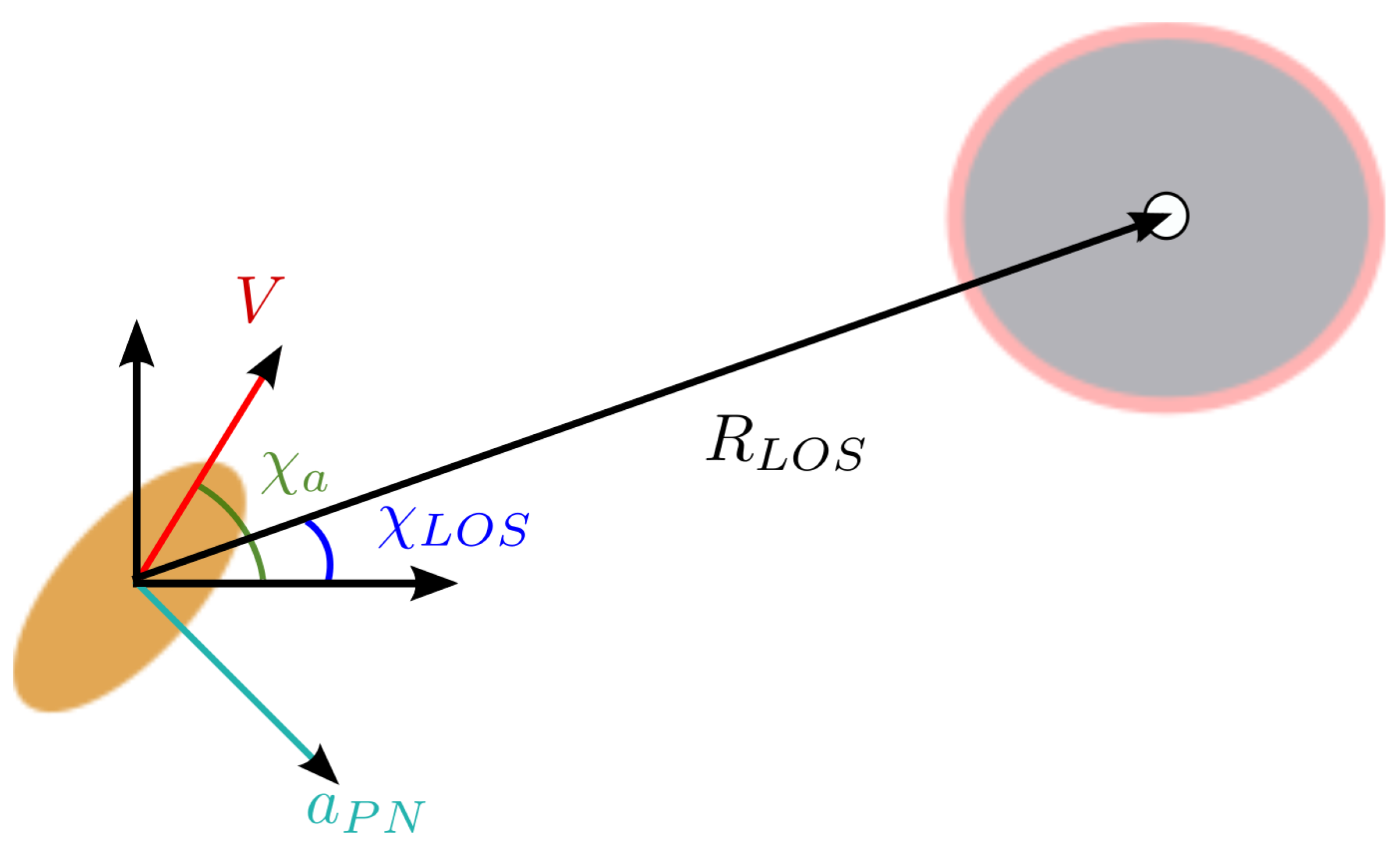
4.2. Proportional Navigation Guidance Law

Proportional navigation (PN) is a method of guidance that has been applied to missiles for terminal guidance [30]. It is one of the most popular guidance methods for short-range intercept [31] and also has been applied to aircraft collision avoidance problems [32]. In this section, a PN guidance law is developed for airship waypoint navigation, where the waypoints are treated as non-moving targets and the airship is guided towards them. Yaw rate commands are generated by the PN law and fed into the LQ controller as reference signals. The reference signal is compared to the airship yaw rate, and the error generates control signals to yaw the airship towards the next waypoint.
  • χ L O S Line-of-sight heading
  • R L O S Line-of-sight vector
  • a P N Commanded acceleration by the PN guidance law
A typical planar pursuit engagement geometry is shown in Figure 3. χ a , χ L O S , R L O S , V and a P N are the airship heading, line-of-sight (LOS) heading, the LOS vector, the airship velocity vector and the commanded acceleration by the PN guidance law. The commanded acceleration is dictated by the PN law to be:
a P N = N χ ˙ L O S V c
where N is the navigation constant with values usually ranging from two to five, χ ˙ L O S is the rate of rotation of the LOS and V c is the airship closing velocity on the waypoint. From the engagement geometry in Figure 3, it can be seen that χ ˙ L O S = V sin ( χ a χ L O S ) R L O S and V c = | | V | | cos ( χ a χ L O S ) . The value of the commanded heading rate for the airship can be calculated from Equation (14), χ ˙ c o m m = a P N V c . To supply the controller with a commanded yaw rate, it is assumed that the commanded heading rate from the PN law is equal to a commanded yaw rate; therefore, ψ ˙ c o m m = χ ˙ c o m m . ψ ˙ c o m m is used as a reference signal in the previously designed LQ controller to force the airship to track the yaw rate commands generated by the PN-law, therefore guiding it through any series of waypoints.

4.3. Gain Scheduling Law

The need for a gain scheduling law arises from the fact that when a controller is designed to work at a specific trim point and the system largely deviates from that point, the controller no longer functions efficiently. Therefore, the controller gains are calculated for multiple trim points, and then, the gain scheduling law is used to interpolate the gain values for specific flight conditions. The proposed gain scheduling law for acquiring the value of the gain matrix for the LQ control laws is K = ( 1 σ K ) K S L + σ K K L T , where σ K is the scheduling parameter, and is a function of a scheduling variable, the turn rate ψ ˙ . The turn rate is selected as a scheduling variable based on the fact that the airship is only required to fly in a straight line towards the current waypoint, and upon breaching the waypoint proximity zone, it would turn towards the next waypoint. This translates into σ K having a value between zero and one, where at σ K = 0 , the airship is flying straight and level, and at σ = 1 , the airship is turning. A linear function is proposed for the scheduling parameter as a function of the scheduling variable in the following form σ K = 1 ψ ˙ S L ψ ˙ L T ψ ˙ + ψ ˙ S L ψ ˙ S L ψ ˙ L T . Since for a straight and level flight, the turn rate is required to be zero, σ K = | ψ | ˙ ψ ˙ L T .
  • K S L Straight and level flight control gains
  • K L T Level turn flight control gains
  • σ K ) Scheduling parameter
  • ψ ˙ L T Level turn flight rate of turn
  • ψ ˙ S L Straight and level flight rate of turn
A saturation limit is imposed, where when the value of | ψ | ˙ is larger than ψ ˙ L T , the value of σ K = 1 . It should be noted that the value of | ψ | ˙ while flying straight and level should, theoretically, be zero. However, due to sensor imperfections, while measuring the turn rate and as a consequence of the dynamics of the closed-loop feedback system, the value of | ψ | ˙ during straight and level flight will not be exactly zero. This causes the scheduling parameter σ K to not strictly be equal to zero during straight and level flight, as well. This generates an interpolated value of the gains during straight and level flight, which in turn introduces additional modeling errors. This effect will also be amplified later on when the estimated values of the states are fed back to the controller from a Kalman filter.

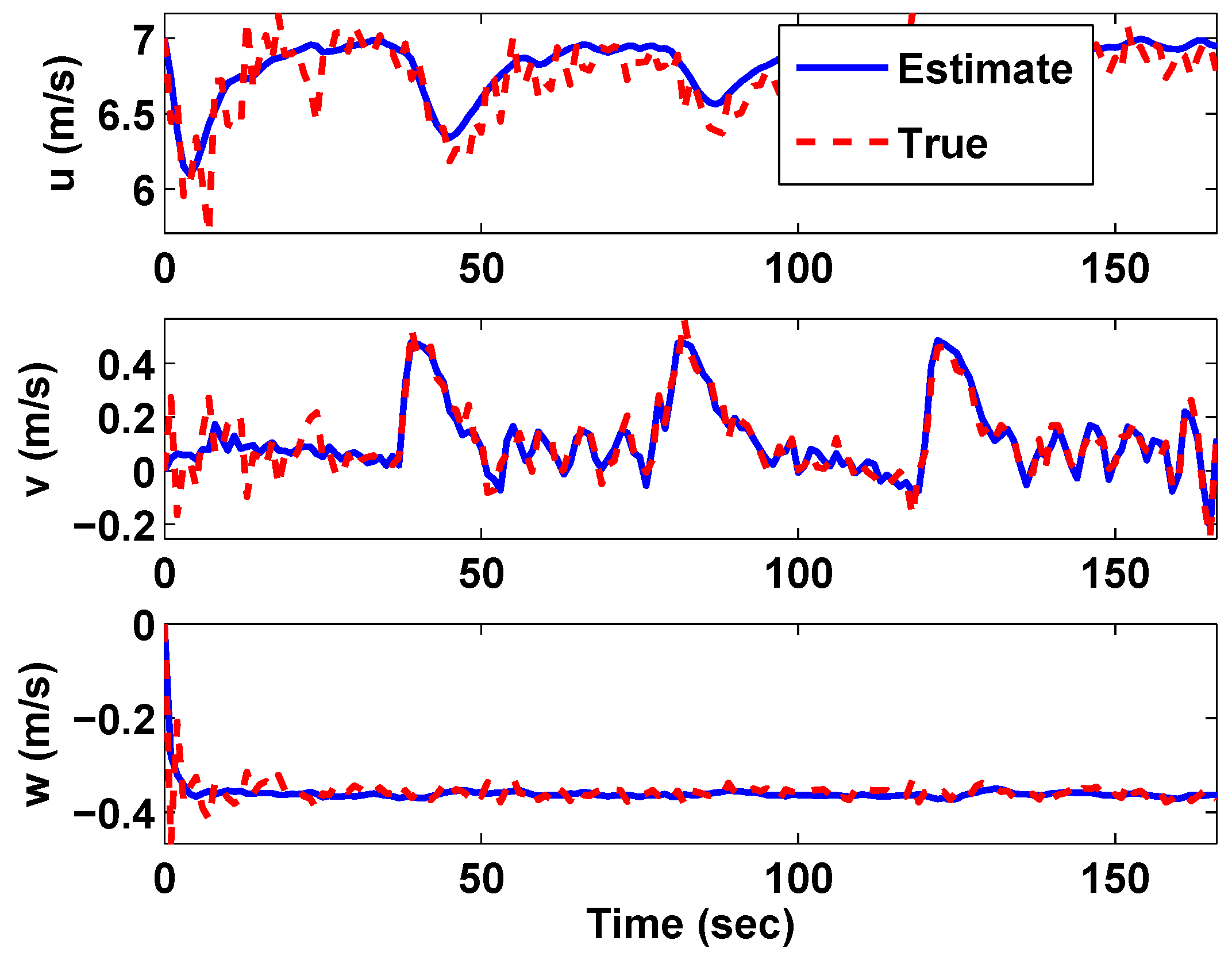
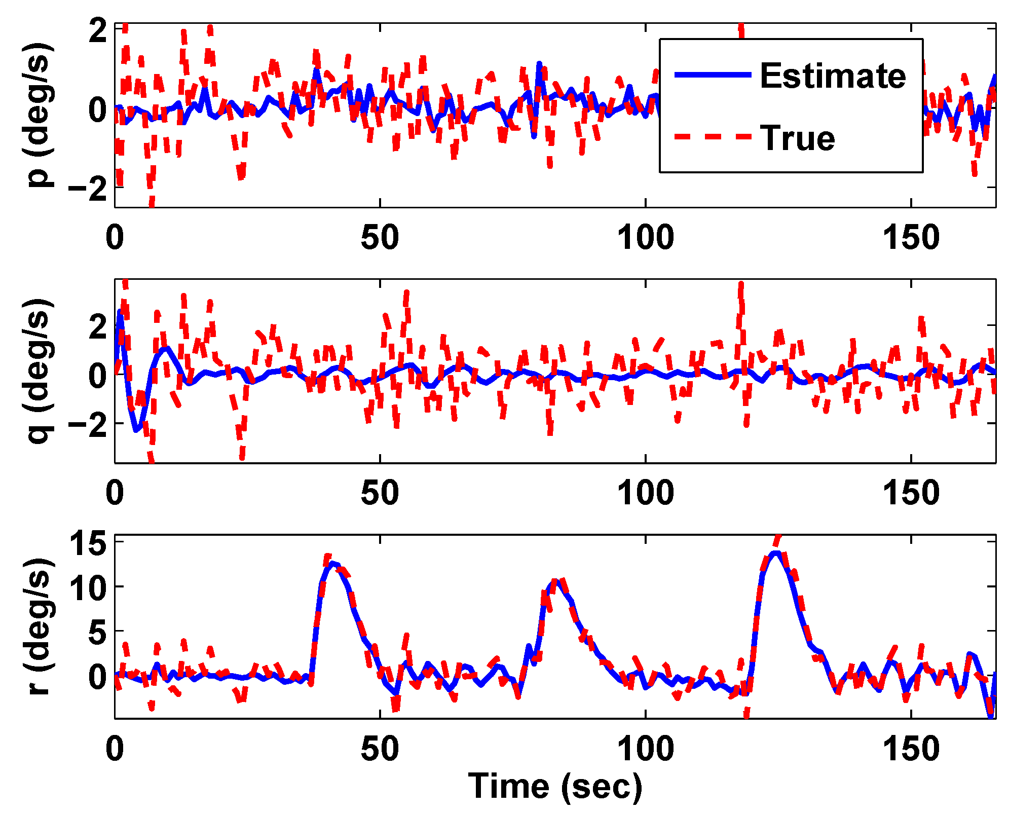
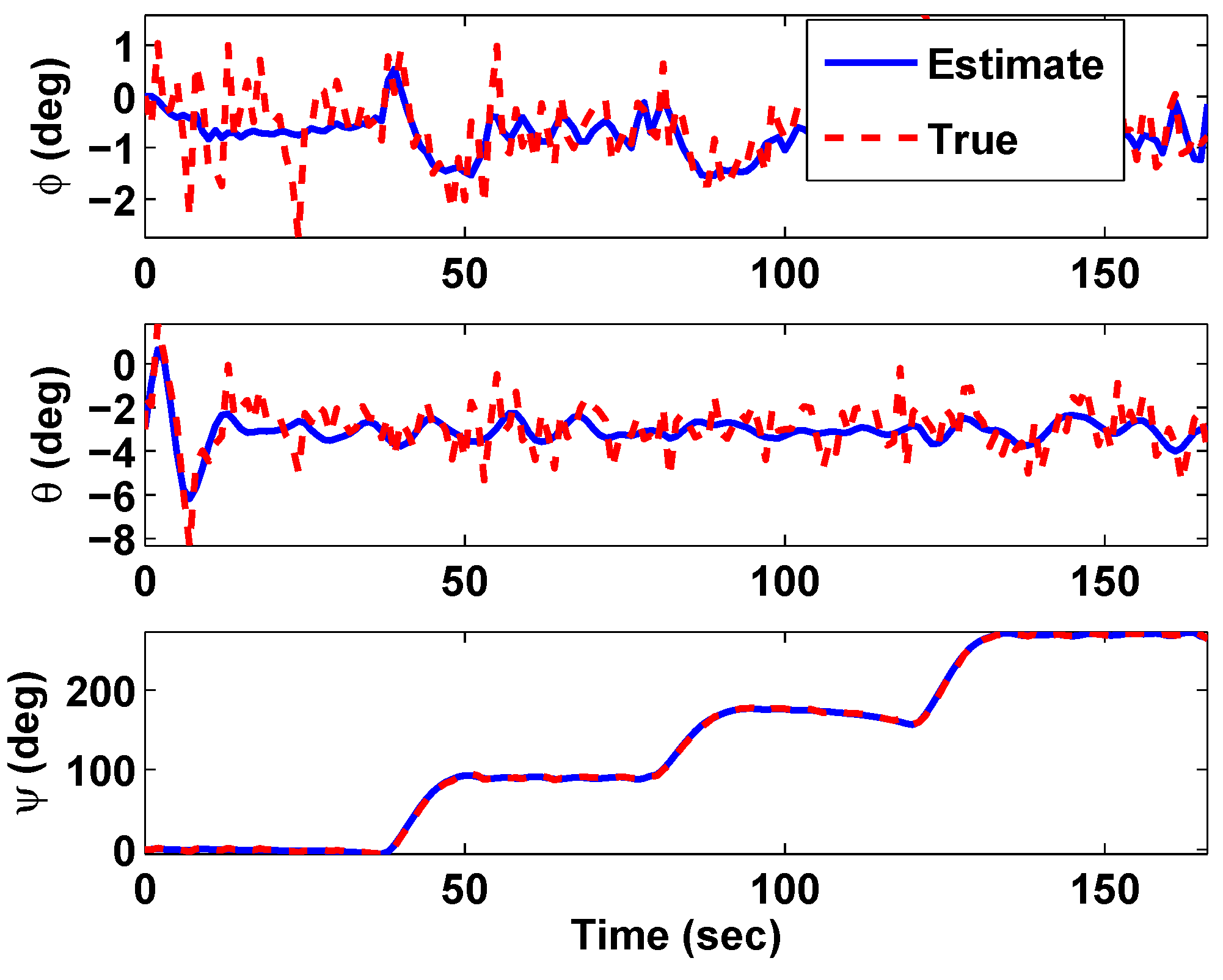
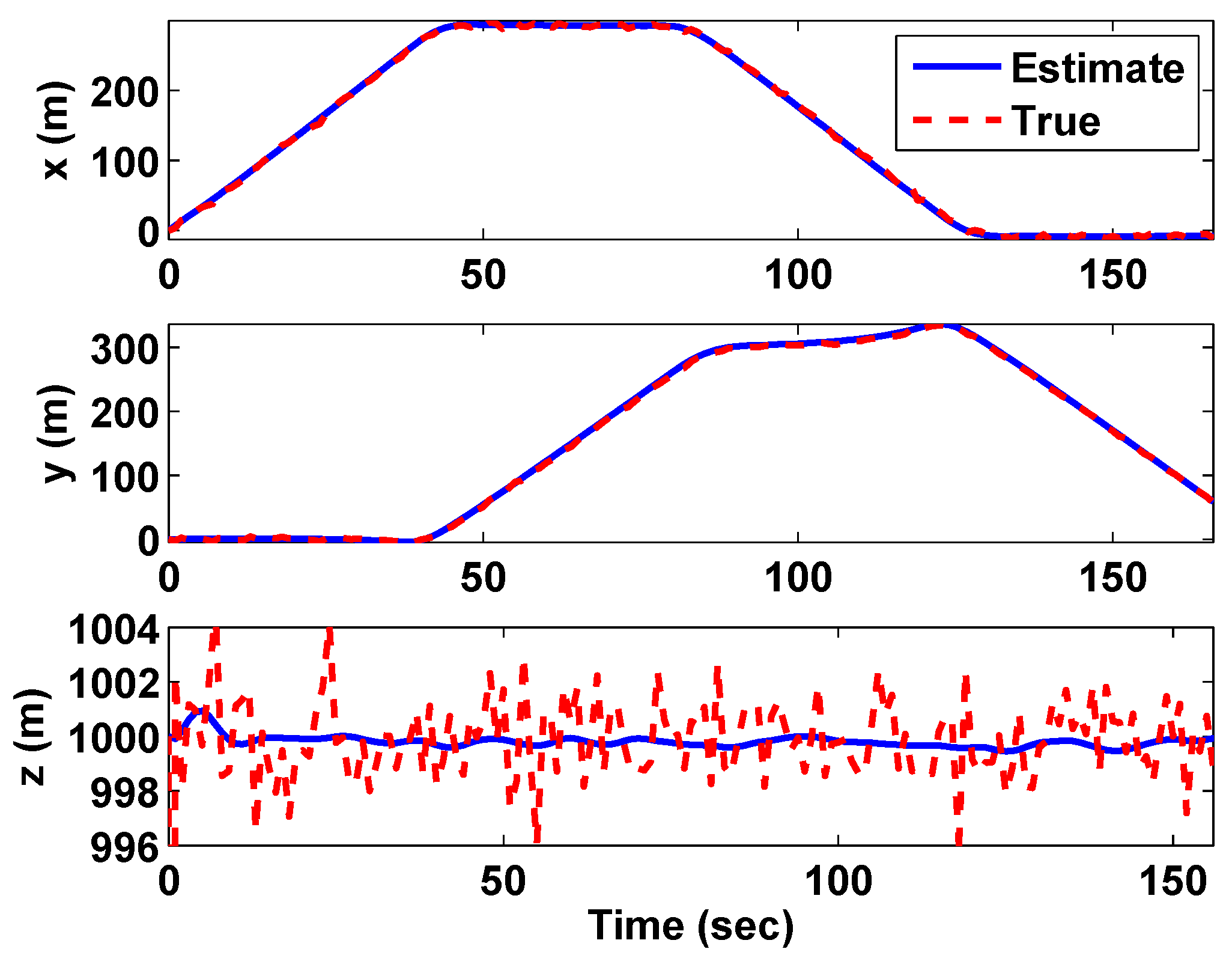
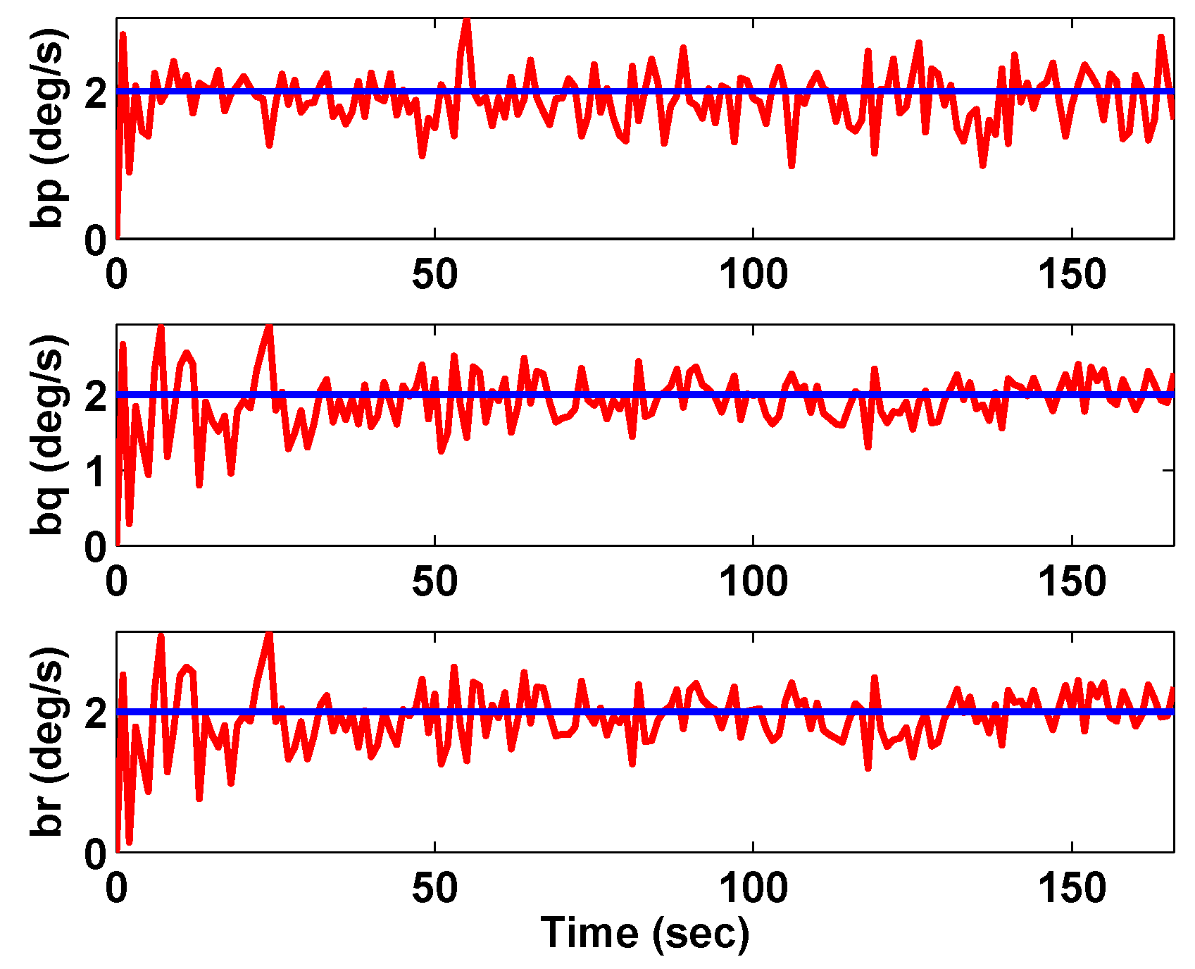
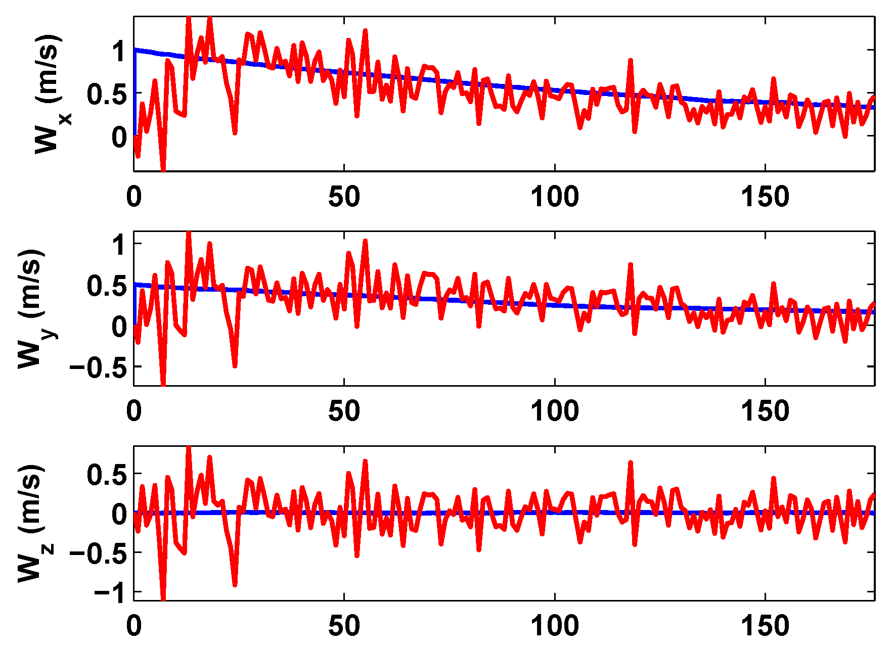
5. State and Wind Estimation Using a Scheduled Extended Kalman Filter

A novel implementation of the scheduled extended Kalman filter (SEKF), with a minimal sensor suite on-board the airship, for estimating the full state vector of the airship along with the wind field in which it is flying, is implemented. Measurements are provided only from an IMU and a GPS sensor. The system Jacobians need not be calculated at every instant and are precalculated for the different flight modes that the airship will encounter. A “Jacobian scheduling law” is introduced to supply the filter with the needed values at every instant of the flight. This version of the filter, referred to as the scheduled extended Kalman filter (SEKF), is shown to work very well, especially when the dynamics does not change very rapidly, with the added advantage of reduced computational effort. The process dynamics is governed by Equations (1)–(5) and can be put in compact form as follows:
X ˙ w = f ( X w , U )
where X w = [ u v w p q r x y z ϕ θ ψ W x W y W z W ˙ x W ˙ y W ˙ z ] T and U = [ T M γ T M T t Δ 1 Δ 2 ] T . The measurements are obtained from the available sensors, i.e., GPS and IMU. No air data sensors are assumed available. Such sensors are available in a conventional suite of on-board UAV avionics [33]. The GPS will provide measurements for the inertial position vector, and the IMU will provide measurements for the angular rates along with the Euler angles. This leads to the following measurement vector:
Y ˜ = [ p ˜ q ˜ r ˜ x ˜ y ˜ z ˜ ϕ ˜ θ ˜ ψ ˜ ] T
  • Y ˜ Measurement vector
Further, the measurements of p , q , r , x , y , z , ϕ , θ and ψ are assumed to be corrupted with bias and zero-mean Gaussian white noise. The bias and white noise standard deviation values are summarized in Table 4.
The state and wind estimates are propagated according to Equation (15) as X ^ ˙ w = f ( X ^ w , U ) with X ^ w representing the estimate of the composite state vector that includes the wind velocity and the wind acceleration estimates.
X ^ w = [ u ^ v ^ w ^ p ^ q ^ r ^ x ^ y ^ z ^ ϕ ^ θ ^ ψ ^ W ^ x W ^ y W ^ z W ^ ˙ x W ^ ˙ y W ^ ˙ z ] T
W ^ ˙ x = b w W ^ x W ^ ¨ x = b w W ^ ˙ x W ^ ˙ y = b w W ^ y W ^ ¨ y = b w W ^ ˙ y W ^ ˙ z = 0 W ^ ¨ z = 0
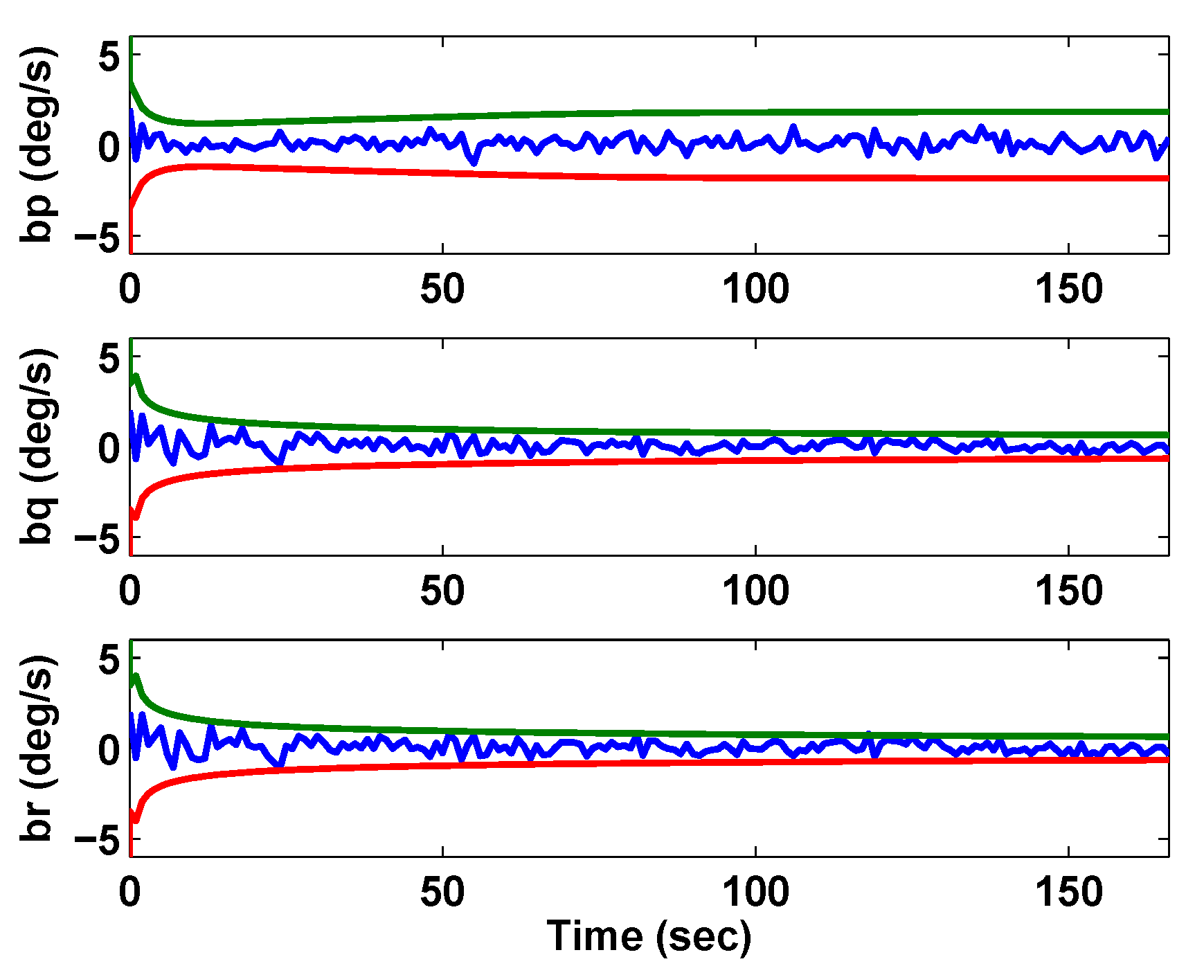
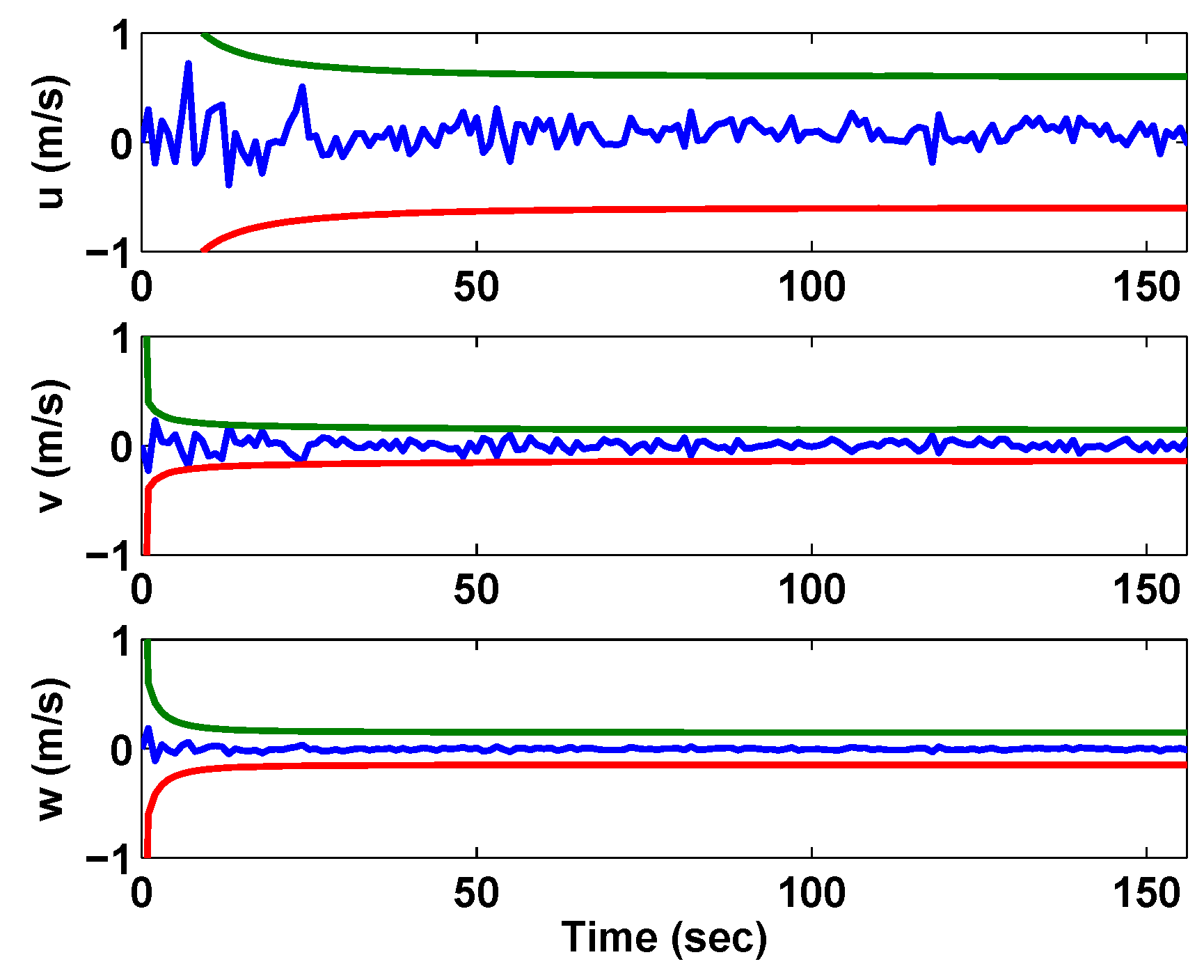
Since the measurement biases are constant, we augment them to the estimator system dynamics equations as,
[ b ^ ˙ p b ^ ˙ q b ^ ˙ r ] T = [ 0 0 0 ] T
where b ^ p , b ^ q and b ^ r are the estimated values of the bias in p ˜ , q ˜ and r ˜ , respectively. The description for the propagation models above leads to an augmented estimated state vector,
X ^ b w = [ u ^ v ^ w ^ p ^ q ^ r ^ x ^ y ^ z ^ ϕ ^ θ ^ ψ ^ W ^ x W ^ y W ^ z W ^ ˙ x W ^ ˙ y W ^ ˙ z b ^ p b ^ q b ^ r ] T
The error covariance matrix is propagated through the continuous-time Riccati equation (Equation (20)); however, the need to calculate the Jacobian F ( x ^ ( t ) , t ) = f x | x ^ k at every instant is computationally expensive and can be a complicated process for highly nonlinear systems. In the SEKF framework, we precalculate the Jacobian at the two trim flight conditions and use the scheduling law proposed for the controller gains presented earlier, to acquire the value of the Jacobian during flight. In this novel implementation of the filter, only the elements pertaining to the change of the linear velocities ( u v w ) and angular rates ( p q r ) with respect to the wind acceleration need to be computed each time. The following “Jacobian scheduling law” is used, F = ( 1 σ K ) F S L + σ K F L T .
P ˙ ( t ) = F P ( t ) + P ( t ) F T + G Q G T
  • F S L Straight and level flight state Jacobian
  • F L T Level turn flight state Jacobian
  • H Measurement Jacobian
  • P Error covariance matrix
where Q is a 15 × 15 diagonal matrix with elements shown in Table 5 and:
G = I 6 × 15 [ 0 ] 6 × 15 [ 0 ] 3 × 6 I 3 × 3 [ 0 ] 3 × 6 [ 0 ] 3 × 9 I 6 × 6
The state estimates and the error covariance are updated every time a measurement is obtained using the Kalman gain from Equation (21). From the measurement model, it is seen that the Jacobian H k T ( x ^ k ) = h x | x ^ k has a constant value for all time.
K k = P k H T [ H P k H T + R k ] 1
where:
H = [ 0 ] 3 × 3 [ I ] 3 × 3 [ 0 ] 3 × 6 [ I ] 3 × 3 [ 0 ] 3 × 6 [ 0 ] 3 × 6 [ I ] 3 × 3 [ 0 ] 3 × 4 [ 0 ] 3 × 4 [ 0 ] 3 × 4 [ 0 ] 3 × 9 [ I ] 3 × 3 [ 0 ] 3 × 3 [ 0 ] 3 × 3 [ 0 ] 3 × 3
and R k is a 9 × 9 diagonal matrix with elements shown in Table 6.
After the Kalman gain has been calculated, the estimate vector and the error covariance matrix are updated as follows:
X ^ k + = X ^ k + K k [ y ˜ k y ^ ( X ^ k ) ] P k + = [ I K k H k ( X ^ k ) ] P k
where y ^ ( X ^ k ) = [ p ^ q ^ r ^ x ^ y ^ z ^ ϕ ^ θ ^ ψ ^ ] T ; X ^ k is the propagated estimate vector in Equation (19), and P k is the propagated value of the error covariance matrix at the previous instant.

6. Results and Discussion

6.1. Flight in Zero Wind Condition

The simulation is initialized with the airship at the origin of the inertial frame; the airship will then travel to four pre-programmed waypoints until it has visited each one. The radius of the waypoint proximity zone around each waypoint is set to 50 m; the altitude is held at 1000 m; and the speed is kept constant at a value of 7 m/s. The simulation is carried out for both guidance laws first without wind effects.
Figure 4, Figure 5, Figure 6 and Figure 7 show the time history of the airship states throughout the simulation. It is noticed from Figure 4 that there are three distinct peaks in the value of the side-speed during the simulation. This is indicative of the airship slipping while turning; this is due to the fact that unlike fixed wing aircraft, since airships generate lift through buoyancy they do not bank to turn. Hence, a side-slip is induced during a turn. Figure 5 shows a zero pitch rate for all simulation time, along with three visible peaks of the yaw rate. These peaks correspond to the turns executed by the airship after arriving at each waypoint.
In Figure 6, it is noticed that while banking in one direction (left, negative), the airship yaws in the other (right, positive). This is explained by the location of the tail thrust source. Since it is located above the center of gravity, the tail thruster induces a “negative” roll moment when operated to generate a “positive” yaw moment. Therefore, yawing the airship to the right induces a negative roll to the left. This is also another illustration of how airship operation differs substantially from conventional aircraft. The altitude of the airship is kept constant by the LQ controller during the simulation. This result can be seen in Figure 7.
Figure 8, Figure 9, Figure 10 and Figure 11 show the time history of the states of the airship while executing a simulation similar to the one whose results are displayed in Figure 4, Figure 5, Figure 6 and Figure 7; however, these results display the achieved output when using the PN guidance law in combination with the LQ controller designed earlier. It is clear from Figure 8 that the airship also undergoes a side-slip while turning; however, this time, the turn is somewhat continuous. This is due to the continuously-generated acceleration commands by the PN guidance law. This can be confirmed by examining the yaw rate (r) in Figure 9, which is non-zero for the entire flight time.
Again, the opposite direction roll phenomenon discussed earlier can also be seen in Figure 10. The inertial position of the airship while guided by the PN guidance law is shown in Figure 11. The path is indicated to be of circular nature, which is again attributed to the mode of operation of a PN guidance law.

6.2. Flight under Time-Varying Wind

North-east wind, generated using the wind model discussed earlier, is introduced into the simulation. The wind inertial speeds can be seen in Figure 12. As a result of the wind presence, the airship flight path, generated from the TS guidance law simulation, is shifted when compared to the no-wind flight path, as shown in Figure 13. The wind effect on the airship dynamics can be substantial in many situations, and this may lead to undesired performance; therefore, this is an issue worthy of solving. This is done by implementing the SEKF designed earlier in order to estimates the wind speed and feed it back to the TS guidance law. This will allow it to generate signals, with knowledge of the wind, to the controller in order to achieve enhanced performance. For the PN guidance law, the trajectory is also shifted, as can be seen in Figure 14. However, since the purpose of the PN law is to reach each waypoint traveling on any trajectory possible, it has less performance constraints; therefore, it is more robust to wind disturbances.
For the next set of results, the SEKF is now implemented in the simulation. First the simulation is run under the zero wind condition to capture the performance of the TS guidance law and LQ controller with the presence of uncertainty in the estimated states. Figure 15, Figure 16, Figure 17 and Figure 18 show the time history of all of the airship states along with their estimates. It is clear that the introduction of uncertainty into the simulation has altered the results. However, the results indicate that the LQ controller is capable of keeping the airship stable and navigating it through the desired waypoints based on the signals from the TS guidance law. It is also noticed that in Figure 15, Figure 16 and Figure 17, there are small amplitude oscillations in lateral states, such as the side-speed, yaw rate and bank angle. These oscillations occur after the airship has executed a turn. This can be attributed to the nature of the gain scheduling law derived earlier. The gain scheduling law is a function of the airship’s turn rate ψ ˙ , which, due to the uncertainties added to the system by measurement noise and bias, does not go back to zero exactly after an airship has executed a turn. The turn rate fed into the gain scheduling law is generated by estimates provided by the Kalman filter, and the fact that it is not perfectly zero causes such oscillations to occur.
The SEKF was also able to estimate the bias in the angular velocity measurements; the result is shown in Figure 19. Error between the estimated value and true value of the bias is shown in Figure 20 along with the three-σ bounds. The estimation errors and three-σ bounds for the body-frame velocity components are also shown in Figure 21. From the figure, it can be stated that the body-frame velocity components are estimated with operationally-acceptable levels of uncertainty; this shows the effectiveness of the implemented SEKF. The three-σ bounds are not shown for all of the estimated states and parameters for brevity; the ones shown however are to serve as an indication of the filter’s convergence.
The same wind field, previously introduced, is integrated into the simulation with the SEKF implementation. Figure 22 shows the true and estimated values of the wind speeds. It is clear that the Kalman filter is capable of estimating the wind speed with acceptable levels of uncertainty, given the minimal number of sensors on-board the airship. This information can now be used to enhance the controller and TS guidance law’s performance. The values of the estimated wind speeds are fed into the TS guidance law in such a way that the inertial velocities used to calculate the vehicle heading can account for the wind information. This enables the TS guidance law to generate more signals that enhance the controller performance in the presence of wind. Examining Figure 23, it can be seen that from both simulations, the performance of the TS guidance law is enhanced when the estimated wind speeds are available at its disposal.

7. Conclusions

From the work presented in this paper on the control of an unmanned airship through waypoint navigation under time-varying wind conditions, we observe that the dynamics of lighter-than-air flight are substantially different from those of conventional heavier-than-air flight in that airship dynamics are significantly affected by wind. A simple LQ controller receiving navigation commands from a track-specific or a proportional navigation guidance law is capable of navigating the AS500 airship through a series of waypoints under zero wind condition and the presence of time-varying wind. A scheduled extended Kalman filter that uses pre-computed system Jacobians works quite well and yields acceptable estimates of the states, measurement biases and prevailing wind while receiving measurements from only the GPS and IMU sensors. It is found that the information of the estimated wind speeds can be used to enhance the guidance commands sent to the LQ controller, which in turn delivers an enhanced performance.

Acknowledgments

The authors wish to acknowledge Atilla Dogan with the University of Texas at Arlington for his notes on the mathematical modeling of the dynamics of airships.

Author Contributions

Kamesh Subbarao conceived the initial problem of the guidance, navigation, and control of airships subject to uncertain wind disturbances. Ghassan Atmeh developed the problem to include wind disturbances, formulate the Scheduled Extended Kalman Filter, and the guidance laws. Ghassan Atmeh also wrote the preliminary version of the paper. Kamesh Subbarao subsequently revised and completed the paper. Ghassan Atmeh performed all the simulations. The two authors jointly performed the analysis.

Conflicts of Interest

The authors declare no conflict of interest.

Appendix A

The aerodynamic force and moment coefficients for the airship are represented based on three different cases that correspond to the deflections of the tail fin aerodynamic surfaces Δ 1 and Δ 2 [20] and are summarized below.
  • When Δ 1 = Δ 2 = 0 :
    C L = 0 . 1226 cos ( α ) sin ( 2 β ) + 0 . 372 sin ( β ) sin ( α ) 2 cos 2 ( β ) + sin 2 ( β ) + 0 . 937 cos ( α ) sin ( 2 β ) + 1 . 855 sin ( β ) sin ( α ) 2 cos 2 ( β ) + sin 2 ( β ) C N = 0 . 024 + 0 . 937 sin ( 2 α ) cos 2 ( β ) + 1 . 855 sin ( α ) cos ( β ) sin 2 ( α ) cos 2 ( β ) + sin 2 ( β ) C T = 0 . 1111 0 . 2045 ( C N + 0 . 2 ) tan α 2 cos 2 ( α ) cos 2 ( β ) C l = 0 . 548 sin ( α ) + 1 . 045 ρ cos ( α ) sin ( 2 β ) ρ S r e f L r e f C m = 0 . 04 0 . 173 sin ( 2 α ) cos 2 ( β ) 1 . 234 sin 2 ( α ) cos 2 ( β ) + sin 2 ( β ) sin ( α ) cos ( β ) C n = 0 . 185 cos ( α ) sin ( 2 β ) + 1 . 165 sin 2 ( α ) cos 2 ( β ) + sin 2 ( β ) sin ( β )
  • When Δ 1 and Δ 2 are of the same sign, δ e q = Δ 1 + Δ 2 2 :
    K 1 = 0 . 0553 0 . 0129 δ e q + 0 . 0488 δ e q 2 K 2 = 0 . 061 0 . 4132 δ e q + 0 . 06899 δ e q 2 1 . 27 δ e q 3 K 3 = 0 . 1069 0 . 0087 δ e q + 0 . 0932 δ e q 2 C L = 0 . 1226 cos ( α ) sin ( 2 β ) + 0 . 372 sin ( β ) sin 2 ( α ) cos 2 ( β ) + sin 2 ( β ) + 0 . 937 cos ( α ) sin ( 2 β ) + 1 . 885 sin ( β ) sin 2 ( α ) cos 2 ( β ) + sin 2 ( β ) C N = 0 . 024 + 0 . 937 sin ( 2 α + 0 . 085 δ e q ) cos 2 ( β ) + 1 . 855 sin ( α + 0 . 085 δ e q ) cos ( β ) sin 2 ( α + 0 . 085 δ e q ) cos 2 ( β ) + sin 2 ( β ) C T = K 1 s i g n C N C N 2 + C L 2 + K 2 2 + K 3 cos 2 ( α ) cos 2 ( β ) C l = 0 . 548 sin ( α ) + 1 . 045 ρ cos ( α ) sin ( 2 β ) ρ S r e f L r e f C m = 0 . 04 0 . 173 sin ( 2 α + 0 . 2 δ e q ) cos 2 ( β ) 1 . 234 sin 2 ( α + 0 . 2 δ e q ) cos 2 ( β ) + sin 2 ( β ) sin ( α + 0 . 2 δ e q ) cos ( β ) C n = 0 . 185 cos ( α ) sin ( 2 β ) + 1 . 165 sin 2 ( α ) cos 2 ( β ) + sin 2 ( β ) sin ( β )
  • When Δ 1 and Δ 2 are of different signs, δ e q = Δ 1 + Δ 2 2 :
    K 1 = 0 . 0553 + 0 . 0129 δ e q + 0 . 0488 δ e q 2 K 2 = 0 . 061 + 0 . 4132 δ e q + 0 . 06899 δ e q 2 + 1 . 27 δ e q 3 K 3 = 0 . 1069 + 0 . 0087 δ e q + 0 . 0932 δ e q 2 C L = 0 . 1226 cos ( α ) sin ( 2 β ) + 0 . 372 sin ( β ) sin 2 ( α ) cos 2 ( β ) + sin 2 ( β ) + 0 . 937 cos ( α ) sin ( 2 β 0 . 085 δ e q ) + 1 . 885 sin ( β 0 . 085 δ e q ) sin 2 ( α ) cos 2 ( β 0 . 085 δ e q ) + sin 2 ( β 0 . 085 δ e q ) C N = 0 . 024 + 0 . 937 sin ( 2 α ) cos 2 ( β ) + 1 . 855 sin ( α ) cos ( β ) sin 2 ( α ) cos 2 ( β ) + sin 2 ( β ) C T = K 1 C N 2 + C L 2 + K 2 2 + K 3 cos 2 ( α ) cos 2 ( β ) C l = 0 . 548 sin ( α ) + 1 . 045 ρ cos ( α ) sin ( 2 β ) ρ S r e f L r e f C m = 0 . 04 0 . 173 sin ( 2 α ) cos 2 ( β ) 1 . 234 sin 2 ( α ) cos 2 ( β ) + sin 2 ( β ) sin ( α ) cos ( β ) C n = 0 . 012 cos ( α ) sin ( 2 β ) 0 . 069 sin ( β ) sin 2 ( α ) cos 2 ( β ) + sin 2 ( β ) + 0 . 173 cos ( α ) sin ( 2 β 0 . 2 δ e q ) + 1 . 234 sin ( β 0 . 2 δ e q ) sin 2 ( α ) cos 2 ( β 0 . 2 δ e q ) + sin 2 ( β 0 . 2 δ e q )
where α and β are the angle of attack and side-slip angle.

Appendix B

The Coriolis-centrifugal coupling matrix as given by [20] is:
D = D 11 D 12 D 13 D 14 D 15 D 16 D 21 D 22 D 23 D 24 D 25 D 26 D 31 D 32 D 33 D 34 D 35 D 36 D 41 D 42 D 43 D 44 D 45 D 46 D 51 D 52 D 53 D 54 D 55 D 56 D 61 D 62 D 63 D 64 D 65 D 66
The virtual mass and inertia matrices are given as:
F 1 = a 11 0 0 0 a 22 0 0 0 a 33
F 2 = 0 0 0 a 24 0 a 26 0 a 35 0
M 1 = a 44 0 a 46 0 a 55 0 a 46 0 a 66
M 2 = 0 a 42 0 0 0 a 53 0 a 62 0
where:
D 11 = 0 D 21 = p m 13 + r ( x m 11 a 11 ) D 31 = ( a 11 x m 22 ) q
D 12 = a 22 r D 22 = 0 D 32 = a 22 p
D 13 = a 33 q D 23 = a 33 p D 33 = 0
D 14 = a 24 r D 24 = a 35 q D 34 = a 24 p a 26 r
D 15 = a 35 q D 25 = a 15 q D 35 = a 15 q
D 16 = a 26 r D 26 = 0 D 36 = 0
D 41 = p m 33 + r ( a 15 + x m 13 ) D 51 = ( a 35 + x 2 m 22 ) q
D 42 = ( a 62 + a 35 ) q D 52 = a 42 r + a 62 p
D 43 = ( a 62 + a 35 ) q + a 24 p D 53 = a 15 q
D 44 = a 64 q D 54 = a 64 p + ( a 66 a 44 ) r
D 45 = ( a 55 a 66 ) r D 55 = 0
D 46 = 0 D 56 = a 64 r
D 61 = ( a 51 + a 24 x m 13 ) p ( a 26 x 2 m 11 ) r
D 62 = ( a 15 + a 42 ) q
D 63 = a 53 p
D 64 = ( a 44 a 55 ) q
D 65 = a 46 r
D 66 = 0
and:
a 11 = 1 . 247 ρ a 22 = 17 . 219 ρ a 26 = 56 . 893 ρ a 35 = 55 . 269 ρ
a 15 = 0 a 24 = 1 . 231 ρ a 33 = 16 . 671 ρ a 42 = a 24
a 44 = 13 . 38 ρ a 51 = a 15 a 55 = 311 . 942 ρ a 64 = a 46
a 46 = 3 . 658 ρ a 53 = a 35 a 62 = a 26 a 66 = 316 . 814 ρ
m 13 = 1 . 045 ρ x m 11 = 20 . 973 ρ x m 22 = 19 . 337 ρ
m 33 = 40 . 573 ρ x m 13 = 3 . 721 ρ x 2 m 11 = 141 . 625
where ρ is the air density.

References

  1. Li, Y. Dynamics Modeling and Simulation of Flexible Airships. Ph.D. Thesis, Department of Mechanical Engineering, McGill University, Montreal, Quebec, Canada, 2008. [Google Scholar]
  2. Gerken, L.C. Airships: History and Technology; AmeraTechReportican Scientific Corp.: Chula Vista, CA, USA, 1990. [Google Scholar]
  3. Kornienko, A. System Identification Approach for Determining Flight Dynamical Characteristics of an Airship from Flight Data. Ph.D. Thesis, Faculty of Aeronautics and Astronautics and Geodesy, University of Stuttgart, Stuttgart, Germany, 2008. [Google Scholar]
  4. Mueller, J.; Paluszek, M. Development of an Aerodynamic Model and Control Law Design for a High Altitude Airship. In Proceedings of the 3rd Unmanned Unlimited Technical Conference, Workshop and Exhibit, Chicago, IL, USA, 20–23 September 2004.
  5. Bueno, S.; Azinheira, J.; Ramos, J.; Paiva, E.; Rives, P.; Elfes, A.; Carvalho, J.; Silveira, G. Project AURORA: Towards an Autonomous Robotic Airship. In Proceedings of the International Conference on Intelligent Robots and Systems, Lausanne, Switzerland, 30 September–4 October 2002.
  6. De Paiva, E.; Bueno, S.; Gomes, S.B.V.; Ramos, J.J.G.; Bergerman, M. A Control System Development Environment for AURORA Semi-Autonomous Robotic Airship. In Proceedings of the International Conference on Robotics and Automation, Demit, MI, USA, 10–15 May 1999.
  7. Carvalho, J.; de Paiva, E.; Azinheira, J.; Ferreira, P.; Ramos, J.; Bueno, S.; Bergerman, M.; Maeta, S.; Mirisola, L.; Faria, B.; et al. Classic and Robust PID Heading Control of an Unmanned Robotic Airship. In Proceedings of the 9th International Symposium on Intelligent Robotic Systems, Toulouse, France, 18–20 July 2001.
  8. Park, C.S.; Lee, H.; Tahk, M.J.; Bang, H. Airship Control Using Neural Network Augmented Model Inversion. In Proceedings of the Conference on Control Applications, Istanbul, Turkey, 25 June 2003.
  9. Moutinho, A.; Azinheira, J.R. Path Control of an Autonomous Airship Using Dynamic Inversion. In Proceedings of the 5th IFAC/EURON Symposium on Intelligent Autonomous Vehicles, Lisbon, Portugal, 5–7 July 2004.
  10. Yan, Z.; Weidong, Q.; Yugeng, X.; Zili, C. Stabilization and Trajectory Tracking of Autonomous Airship’s Planar Motion. J. Syst. Eng. Electron. 2008, 19, 974–981. [Google Scholar] [CrossRef]
  11. Repoulias, F.; Papadopoulos, E. Robotic Airship Trajectory Tracking Control Using a Backstepping Methodology. In Proceedings of the International Conference on Robotics and Automation, Pasadena, CA, USA, 19–23 May 2008.
  12. Melbous, A.; Tami, Y.; Guessoum, A.; Hadjsadok, M. UAV Controller Design and Analysis Using Sliding Mode Control. J. Autom. Syst. Eng. 2010, 4. [Google Scholar] [CrossRef]
  13. Avenant, G. Autonomous Flight Control System for an Airship. M.S. Thesis, Stellenbosch University, Stellenbosch, South Africa, 2010. [Google Scholar]
  14. Dorato, P.; Abdallah, C.; Cerone, V. Linear-Quadratic Control: An Introduction; Prentice Hall Inc.: Englewood Cliffs, NJ, USA, 1995. [Google Scholar]
  15. Masar, I.; Stohr, E. Gain Scheduled LQR Control for an Autonomous Airship. In Proceedings of the 18th International Conference on Process Control, Bratislava, Slovakia, 14–17 June 2011.
  16. Nakpiam, J. Control of Airship Motion in Presence of Wind. M.S. Thesis, Department of Mechanical and Aerospace Engineering, The University of Texas at Arlington, Arlington, TX, USA, 2011. [Google Scholar]
  17. Lacroix, S.; Il, K.J. High Resolution Terrain Mapping with an Autonomous Blimp. In Proceedings of the International Conference on Intelligent Robots and Systems, Luasanne, Switzerland, 30 September–4 October 2002.
  18. Hygounenc, E.; Il, K.J.; Soueres, P.; Lacroix, S. The Autonomous Blimp Project of LAAS-CNRS: Achievements in Flight Control and Terrain Mapping. Int. J. Robot. Res. 2004, 23, 473–511. [Google Scholar] [CrossRef]
  19. Waishek, J.; Dogan, A.; Bestaoui, Y. Investigation into the Time Varying Mass Effect on Airship Dynamics Response. In Proceedings of the Aerospace Sciences Meeting Including th New Horizons Forum and Aerospace Exposition, Orlando, FL, USA, 5–8 January 2009.
  20. Waishek, J.; Dogan, A. Comprehensive Characterization of Airship Response to Wind and Time Varying Mass. In Proceedings of the Atmospheric Flight Mechanics Conference, Toronto, ON, Canada, 2–5 August 2010.
  21. Waishek, J. Derivation of the Dynamics Equations for an Aircraft in Aerial Refueling. M.S. Thesis, Department of Mechanical and Aerospace Engineering, The University of Texas at Arlington, Arlington, TX, USA, 2007. [Google Scholar]
  22. Atmeh, G. Guidance and Control of Unmanned Airships for Waypoint Navigation in the Presence of Wind. M.S. Thesis, University of Texas at Arlington, Arlington, TX, USA, 2012. [Google Scholar]
  23. Lee, J.H.; Dogan, A.; Hullender, D. Estimation of Aircraft States and Wind Exposure. In Proceedings of the Guidance, Navigation, and Control Conference, Portland, OR, USA, 8–11 August 2011.
  24. Elgerd, O.I. Control Systems Theory; McGraw-Hill: New York, NY, USA, 1966. [Google Scholar]
  25. Franklin, G.F.; Powell, J.D.; Emami-Naeini, A. Feedback Control Systems; Prentice-Hall: Upper Saddle River, NJ, USA, 2002. [Google Scholar]
  26. Oral, O.; Cetin, L.; Uyar, E. A Novel Method on Selection of Q and R Matrices in the Theory of Optimal Control. Int. J. Syst. Control 2010, 1, 84–92. [Google Scholar]
  27. Bryson, A.E., Jr.; Ho, Y.-C. Applied Optimal Control; Hemisphere Publishing Corporation: Washington, DC, USA, 1975. [Google Scholar]
  28. Flores, G.; Lugo, I.; Lozano, R. A nonlinear path-following strategy for a fixed-wing MAV. In Proceedings of the International Conference on Unmanned Aircraft Systems (ICUAS), Atlanta, GA, USA, 28–31 May 2013; pp. 1014–1021.
  29. Lugo, I.; Flores, G.; Salazar, S.; Lozano, R. Dubins path generation for a fixed wing UAV. In Proceedings of the International Conference on Unmanned Aircraft Systems (ICUAS), Orlando, FL, USA, 27–30 May 2014; pp. 339–346.
  30. Shukla, U.; Mahapatra, P. The Proportional Navigation Delemma - Pure or True? IEEE Trans. Aerosp. Electron. Syst. 1990, 26, 382–392. [Google Scholar] [CrossRef]
  31. Lu, P. Intercept of Nonmoving Targets at Arbitrary Time-Varying Velocity. J. Guidance Control Dyn. 1998, 21, 176–178. [Google Scholar] [CrossRef]
  32. Han, S.C.; Bang, H.; Yoo, C.S. Proportional Navigation-Based Collision Avoidance for UAVs. Int. J. Control Autom. Syst. 2009, 7, 553–565. [Google Scholar] [CrossRef]
  33. Petrich, J.; Subbarao, K. On-Board Wind Speed Estimation for UAVs. In Proceedings of the Guidance, Navigation, and Control Conference AIAA, Portland, OR, USA, 8–11 August 2011.
Figure 1. Schematic drawing showing the main components of the AS500 airship (not to scale): (a) hull; (b) tail fins.
Aerospace 03 00008 g001
Figure 2. Illustration of the track-specific guidance law methodology.
Aerospace 03 00008 g002
Figure 3. Engagement geometry for planar pursuit of a waypoint.
Aerospace 03 00008 g003
Figure 4. Time history of velocity vector components in the body frame: track-specific (TS) guidance (no wind).
Aerospace 03 00008 g004
Figure 5. Time history of angular velocity vector components in the body frame: TS guidance (no wind).
Aerospace 03 00008 g005
Figure 6. Time history of airship roll, pitch and yaw angles: TS guidance (no wind).
Aerospace 03 00008 g006
Figure 7. Time history of airship inertial position: TS guidance (no wind).
Aerospace 03 00008 g007
Figure 8. Time history of velocity vector components in the body frame: proportional navigation (PN) guidance (no wind).
Aerospace 03 00008 g008
Figure 9. Time history of angular velocity vector components in the body frame: PN guidance (no wind).
Aerospace 03 00008 g009
Figure 10. Time history of airship roll, pitch and yaw angles: PN guidance (no wind).
Aerospace 03 00008 g010
Figure 11. Time history of airship inertial position: PN guidance (no wind).
Aerospace 03 00008 g011
Figure 12. Time-varying wind field.
Aerospace 03 00008 g012
Figure 13. Airship flight trajectory in both no wind and time-varying wind conditions: TS guidance.
Aerospace 03 00008 g013
Figure 14. Airship flight trajectory in both no wind and time-varying wind conditions: PN guidance.
Aerospace 03 00008 g014
Figure 15. Velocity vector components and their estimates in the body frame: TS guidance (no wind).
Aerospace 03 00008 g015
Figure 16. Angular velocity vector components and their estimates in the body frame: TS guidance (no wind).
Aerospace 03 00008 g016
Figure 17. Airship roll, pitch, and yaw angles and their estimates: TS guidance (no wind).
Aerospace 03 00008 g017
Figure 18. Airship inertial position, true and estimated: TS guidance (no wind).
Aerospace 03 00008 g018
Figure 19. Angular rate measurement bias: true and estimate.
Aerospace 03 00008 g019
Figure 20. Angular rate measurement bias estimation error and three-σ bounds.
Aerospace 03 00008 g020
Figure 21. Velocity vector components estimation error and three-σ bounds.
Aerospace 03 00008 g021
Figure 22. Wind velocity estimates.
Aerospace 03 00008 g022
Figure 23. Wind velocity estimates feedback effect on TS guidance law performance.
Aerospace 03 00008 g023
Table 1. AS500 airship physical parameters.
ParameterValue
Net mass21 kg
Surface area2.8352 m2
Length7.8 m
Volume15 m3
Maximum speed12.5 m/s
Table 2. Wind model parameters.
ParameterValue
bw0.0063 s−1
E{W}0 m/s
σw0.5 m/s
Table 3. Trim states.
State/InputStraight and LevelLevel Turn
u (m/s)6.996.98
v (m/s)00.194
w (m/s)−0.365−0.364
p (deg/s)00.27
q (deg/s)0−0.02
r (deg/s)05
z (m)−1000−1000
φ (deg)0−0.8
θ (deg)−3−3
TM (N)10.210.5
γ T M (deg)36.435.6
Tt (N)0.21.7
Δ1 (deg)20−3.7
Δ2 (deg)2020
Table 4. Standard deviations and bias of the measurement vector.
Measurement p ˜ (deg/s) q ˜ (deg/s) r ˜ (deg/s) ϕ ˜ (deg/s) θ ˜ (deg/s) ψ ˜ (deg/s) x ˜ (m) y ˜ (m) z ˜ (m)
SD111111333
Bias222000000
Table 5. Q diagonal elements.
Q i , i Value Q i , i Value
Q 1 , 1 1e-2 Q 9 , 9 1e-6
Q 2 , 2 1e-2 Q 10 , 10 1e-6
Q 3 , 3 1e-2 Q 11 , 11 1e-6
Q 4 , 4 1e-2 Q 12 , 12 1e-6
Q 5 , 5 1e-2 Q 13 , 13 1e-6
Q 6 , 6 1e-2 Q 14 , 14 1e-6
Q 7 , 7 1e-6 Q 15 , 15 1e-6
Q 8 , 8 1e-6
Table 6. R diagonal elements.
R i , i Value R i , i Value R i i Value
R 1 , 1 ( π / 180 ) 2 R 4 , 4 3 2 R 7 , 7 ( π / 180 ) 2
R 2 , 2 ( π / 180 ) 2 R 5 , 5 3 2 R 8 , 8 ( π / 180 ) 2
R 3 , 3 ( π / 180 ) 2 R 6 , 6 3 2 R 9 , c 9 ( π / 180 ) 2

