Trajectory Management of the Unmanned Aircraft System (UAS) in Emergency Situation

Abstract

Unmanned aircraft must be characterized by a level of safety, similar to that of manned aircraft, when performing flights over densely populated areas. Dangerous situations or emergencies are frequently connected with the necessity to change the profiles and parameters of a flight as well as the flight plans. The aim of this work is to present the methods used to determine an Unmanned Aircraft System’s (UAS) flight profile after a dangerous situation or emergency occurs. The analysis was limited to the possibility of an engine system emergency and further flight continuing along a trajectory of which the shape depends on the type of the emergency. The suggested method also enables the determination of an optimal flying trajectory, based on the territory of a special protection zone (for example, large populated areas), in the case of an emergency that would disable continuation of the performed task. The method used in this work allows researchers, in a simplified way, to solve a variation task using the Ritz–Galerkin method, consisting of an approximate solution of the boundary value problem to determine the optimal flight path. The worked out method can become an element of the on-board system supporting UAS flight control.

1. Introduction

Initially, unmanned aircraft (UA) were mainly used for military purposes. When performing missions over the areas of military operations, their task was air recognition. In these special conditions, high reliability and safety were not necessarily required. Today, unmanned aircraft find wider uses. They perform flights over civil territories, both on military and civil missions (border patrol, fire-fighting support, control of areas hit by natural disasters, and so on). Performing flights over densely populated areas, unmanned aircraft must be have a level of safety that is similar to that of manned aircraft.

Contemporary UAs have to be designed considering the established parameters of a flight and performance characteristics that have a direct connection to flight operating safety. The flight operation safety of a UAS should be understood as a level of adjustment of the system of aircraft behavior, co-existing objects, and the environment in which a flight task is performed. Flight operating safety and effectiveness of using the UA are the two basic requirements concerning UAS. When performing a flight, flight safety is endangered by particular situations that cause change to regular operation of the UA. Dangerous situations or emergencies are frequently connected with the necessity to change the schedule, profile, and parameters of a flight.

The aim of this work is to present a method used to determine a UA’s flight profile after a dangerous situation or emergency occurs. The analysis was limited to the possibility of an engine system emergency and further flight continuing along a trajectory of which the shape depends on the type of the emergency. Three possible scenarios in which an emergency takes place were examined:

-

It does not influence the performance of the engine system, however, it limits the time for the UA to get to a destination or an alternative aerodrome.

-

It causes a partial loss of performance (power) of the engine system, which necessitates performing a horizontal flight or a flight with a small altitude loss.

-

It causes complete power loss, which necessitates performing a gliding flight only.

The suggested method also enables the determination of the optimal flying trajectory from the territory of a special protection zone (for example, large populated areas), in the case of an emergency which disables continuation of the performed task.

The problem of optimal control of the aircraft, especially optimization of the flight trajectory, have been described by many authors [1,2,3,4,5,6]. The problem was formed as an alternative question, in which the quality functional, such as flight time, consumed fuel, or other factors, was minimized. However, the boundary conditions and limitations imposed on the aircraft trajectory were accomplished. In order to find a solution, the techniques of dynamic programming, established by Bellman [7], and the Maximum Pontryagin principle [8] were used.

The method used in this work allows researchers to solve a variation task using the Ritz–Galerkin method consisting of an approximate solution of the boundary value problem to determine the optimal flight path [9]. The method allows for the determination of the optimal flight trajectory that fulfils boundary value conditions and limitations imposed on it. The simplified algorithm of optimization uses third degree polynomials to approximate the changes of the selected parameters of the flight.

2. Problem Formulation

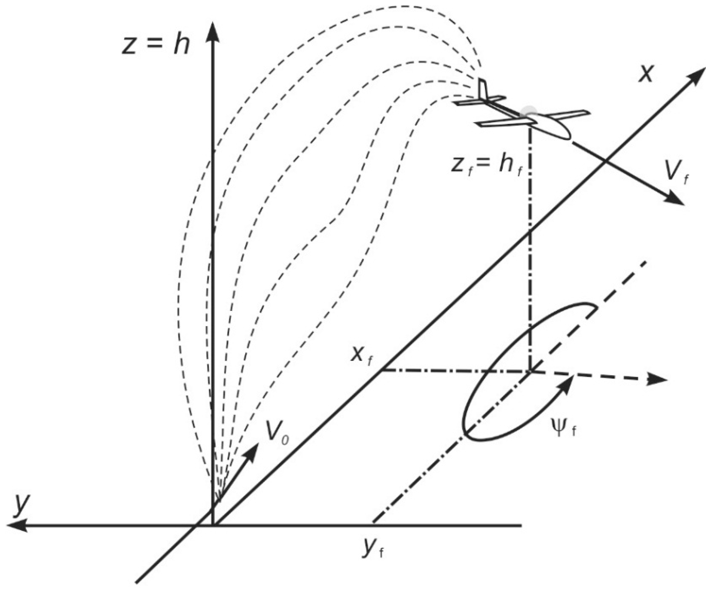
Any task of flight dynamics, consisting of determining the aircraft’s trajectory based on a point mass model, can be formulated as follows: it is necessary to find a control of the aircraft which can guarantee its transition from the initial point of the trajectory, defined by the initial coordinates, to the final point of the trajectory, defined by the final coordinates. An infinite number of trajectories can be drawn between the initial and the final point (Figure 1) and for this reason it can be stated that there are an infinite number of control functions that would provide a solution to the task formulated above. Each set of control functions, which meet the above-mentioned condition, is one of the variants of the solution to the task formulated in such a way. As is known, the movement of the aircraft’s center of gravity in the air is described by a set of seven nonlinear differential equations [9,10], which, in a general case, do not have an analytical solution. Thus, the solution can only be arrived at using numerical methods, defining the boundary conditions for the state variables. However, how to determine the control functions is not known. One of the methods is the selection of the control functions so that a certain quality functional, which depends on state variables and control functions, would reach an extreme value (most often minimal). In this way, the task of finding the flight trajectory of the aircraft comes down to the optimization of the quality functional.

Figure 1. Trajectory optimization problem.

Figure 1. Trajectory optimization problem.

The task of this work is to determine flight parameters of a UA performing flights to an airport or landing field in the aspect of minimal value of the defined functional, depending on the analyzed scenario of events. Set up in such a way, the problem is a complex task and it requires the consideration of a large number of factors. The value of the adopted criteria factor is influenced by a number of factors, such as height and speed of flight, range of engine(s) work, time of the flight, and weather conditions. The method allows prediction of the UA’s trajectory using a point-mass model, describing the forces applied to the center of gravity. This model is formulated as a set of differential algebraic equations (Equation (7)) that must be integrated over a time interval. The control can be performed in two ways: by pulling the control device or changing the range of the engine performance. The first way enables pitching, yawing and rolling. The second way is to change the rotation speed of the engine, as this allows the selection of a proper thrust level. Optimization, thus, is provided to determine such a principle of control of the aircraft so that the curve at which the aircraft moves is extreme. The problem is, therefore, a typical alternative task and the obtained curve is called extreme. There are two main types of these tasks: The first one is when all the values of the determined functions in the initial and final point should be strictly determined. This is the task with determined boundary conditions. In practical tasks of flight dynamics, only some of these conditions are given. These are the so-called tasks with free ends. The analyzed case is an example of such a task. However, although all the conditions are given at only the initial point, some of them are given at the final point. The initial conditions correspond to the initial state of the flight, which follows from the moment when the decision to abort the task performance is made. As far as the final conditions are concerned, some variants can be taken into consideration. The most general is when only one variable is determined (for example, the distance to the place of landing), and the rest of them are resultants. Most frequently, however, the condition will be formed in order to finish a flight at a given height h_f and speed V_f, which, for example, can follow from the conditions of performing a safe landing. Assuming the final time t_f, it is possible to avoid exceeding the maximal time of the flight following, for example, from the amount of accumulated energy in the accumulator (in the case of alternator or main accumulator damage).

It is noteworthy that not all the parameters can change arbitrarily; in order to obtain an optimal trajectory, some of them could exceed their allowed values. That is why the trajectory obtained as a result of optimization should be imposed by certain limitations according to the required principles and instructions of exploitation. Generally these limitations will concern aerodynamics, durability, performance, and those depending on the trajectory shape. Aerodynamic and durability limitations are the most important ones, as they guarantee safe exploitation. They should be considered together because in they are determined simultaneously regarding the durability of the construction and the aerodynamic properties of the airframe, as well as performance characteristics, which take into account the possibility of an emergency. Besides being an acceptable value that cannot be exceeded it is assumed with a certain margin. Under the character of criteria, the following factors are taken into consideration:

-

durability of the airframe construction, engines, and other elements of the aircraft,

-

controllability and stability of the aircraft,

-

phenomena connected with low and high flight speeds (stall, aerodynamic phenomena, etc.),

-

performance limitations (e.g., absolute ceiling),

-

influence of a stormy atmosphere,

-

change of the performance caused by different emergencies (limitation of the power proceeded by the power unit, limitation of the time of the power unit work, complete power loss, etc.).

In the analyzed case, the following limitations are assumed: not exceeding the maximal flight speed, allowable load factor, and allowable angle of attack.

The limitations, depending on the shape of the flight trajectory, take into consideration the range of the flight altitude, which is possible to use regarding the movement, minimal altitude over the ground, avoiding forbidden or dangerous zones, etc.

A general stating of the task supposes determination of the optimal trajectory of movement of a UA (Figure 1) described by the system of ordinary differential equations:

$$x_i=f_i\left(x_1,\dots ,x_n,u_1,\dots ,u_m\right),i=1,2,\dots ,n,m\le n$$

(1)

fulfilling boundary conditions:

$$\begin{array}{l}x\left(t_0\right)=\left\{x_1\left(t_0\right),x_2\left(t_0\right),\dots ,x_n\left(t_0\right)\right\},x\in {\mathbf{\text{R}}}^n\\ x\left(t_f\right)=\left\{x_1\left(t_f\right),x_2\left(t_f\right),\dots ,x_n\left(t_f\right)\right\}\end{array}$$

(2)

and constraints for state variables and control variables:

$$\begin{array}{l}{x}_{i\min }\left(t\right)\le x_i\left(t\right)\le x_{i\max }\left(t\right)\\ u_{j\min }\left(t\right)\le u_j\left(t\right)\le u_{j\max }\left(t\right),j=1,2,\dots ,m\end{array}$$

(3)

where: x_i—state variables; u_j—control variables; t₀, t_f—initial and final times.

The technical characteristics of the flying vehicle are known and can be written as:

$$x_T=\left(x_{T1},\dots ,x_{Tr}\right),x_r\in {\mathbf{\text{R}}}^r$$

(4)

The optimal trajectory x(t), t∈(t₀, t_f) has to be found that minimizes the functional:

$$J\left(x\left(t\right)\right)={\displaystyle \underset{t_0}{\overset{t_f}{\int }}{f}_0\left(X,U\right)dt}$$

(5)

and the control corresponding to it is:

$$U\left(t\right)=\left(u_1\left(t\right),\dots ,u_m\left(t\right)\right),U\in {\mathbf{\text{R}}}^m$$

(6)

In the case of the current task, the system of differential Equation (1), commonly employed in aircraft trajectory analysis, is the following six-dimension system derived at the center of mass of the aircraft [10]:

$$\begin{array}{l}\stackrel{°}{\left(a\right)V}=g\left(\frac{T\cos \text{α}-D}{mg}-\sin \text{γ}\right)\\ \stackrel{°}{\left(b\right)\text{\hspace{1em}γ}}=\frac{1}{mV}\left(\left(T\sin \text{α}+L\right)\cos \text{φ}-mg\cos \text{γ}\right)\\ \left(c\right)\stackrel{°}{\text{\hspace{1em}ψ}}=\frac{\left(T\sin \text{α}+L\right)\sin \text{φ}}{mV\cos \text{γ}}\\ \left(d\right)\stackrel{°}{m}=\frac{dm}{dt}=C_S\\ \left(e\right)\stackrel{°}{x}=V\cos \text{γ}\cos \text{ψ},\left(f\right)\stackrel{°}{y}=V\cos \text{γ}\sin \text{ψ},\left(g\right)\stackrel{°}{z}=\stackrel{°}{h}=V\sin \text{γ}\end{array}$$

(7)

V, γ, ψ, α and φ are, respectively, the speed, the angle of descent, the yaw angle, the angle of attack, and the roll angle. (x, y, z = h) is the position of the aircraft. T, D, L, m (technical characteristics in Equation (4)) and g are the engine thrust, the drag force, the lift force, the aircraft mass, and the gravitational acceleration, respectively. For finding aircraft trajectory purposes, it is commonly assumed to consider a three Degree Of Freedom (DOF) dynamic model that describes the point variable-mass motion of the aircraft over a flat earth model. A standard atmosphere is defined with ISA (International Standard Atmosphere). Lift coefficient C_L is, in general, a function of the angle of attack α and the Mach number M, i.e., C_L = C_L(α,M). The lift coefficient is used as a variable rather than the angle of attack. The aircraft performance model was calculated on the basis of [11,12,13,14,15,16].

There is a relationship between the variables from Equations (1) and (7):

$$x_1=V,x_2=\text{γ},x_3=\text{ψ},x_4=m,x_5=x,x_6=y,x_7=h$$

(8)

The boundary conditions are written in the following way:

$$\begin{array}{l}t=0,x\left(0\right)=x_0,y\left(0\right)=y_0,h\left(0\right)=h_0,\\ V\left(0\right)=V_0,\text{\hspace{0.17em}γ}\left(0\right)={\text{γ}}_0,\text{\hspace{0.17em}ψ}\left(0\right)={\text{ψ}}_0,m\left(0\right)=m_0\\ t=t_f,x\left(t_f\right)=x_f,y\left(t_f\right)=y_f,h\left(t_f\right)=h_f,\\ V\left(t_f\right)=V_f,\text{\hspace{0.17em}γ}\left(t_f\right)={\text{γ}}_f,\text{\hspace{0.17em}ψ}\left(t_f\right)={\text{ψ}}_f,m\left(t_f\right)=m_f\end{array}$$

(9)

As well as the conditions written above, it is necessary to determine the boundary conditions for the control variables:

$$\begin{array}{l}t=0,\text{\hspace{1em}γ}={\text{γ}}_0,T=T_0,\text{\hspace{1em}α}={\text{α}}_0\\ t=t_f,\text{\hspace{1em}γ}={\text{γ}}_f,T=T_f,\text{\hspace{1em}α}={\text{α}}_f\end{array}$$

(10)

3. Method of Taking into Account of Limitations

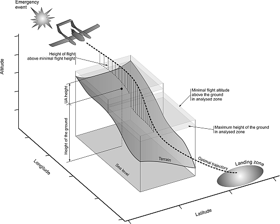
In the process of calculations, the necessity to take into account the limitations imposed on the phase coordinates and steering functions appears several times. The described method allows imposing limitations on the phase coordinates in a simple way. The necessity to impose the limits of that type follows, for instance, from the conditions of the flight performance. In the case of performing the flight at a small altitude, especially when the power unit does not work, a minimal vertical separation from the territory should be provided. In the process of calculations, whether the whole flight trajectory is above the surface should be checked, which determines minimal flight altitude above the ground. The principle of how to determine the flight altitude above the ground is shown in Figure 2.

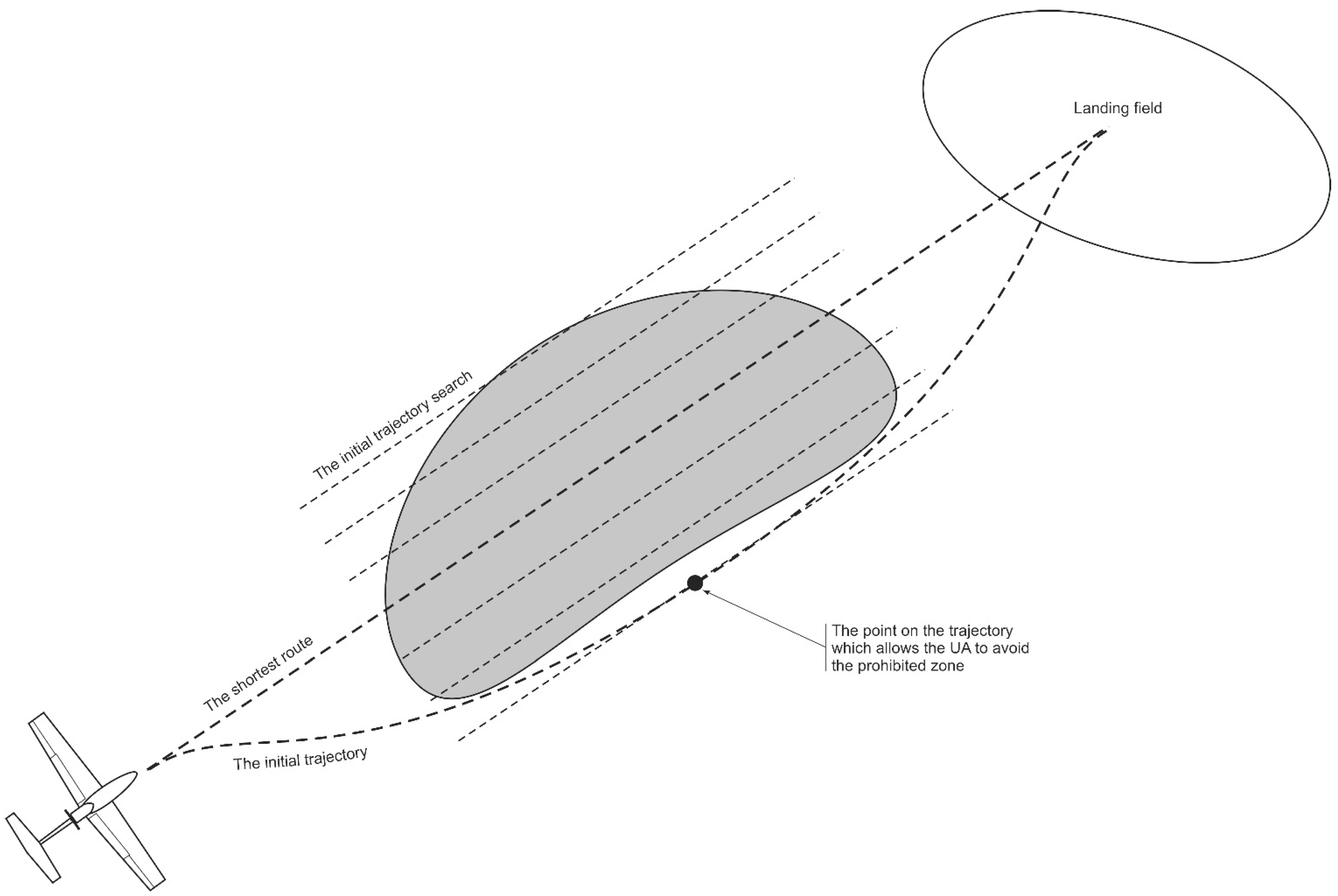
Another limitation is avoidance of the forbidden or dangerous areas. Performing a flight over waters (a lake), in the case of partial operating features loss (emergency), is connected with the risk of necessity to land on the water surface. In the case of a manned aircraft landing on water, it is very dangerous for the life and health of the people on-board. In the case of an unmanned aircraft, main risks are connected with damage and loss of valuable devices that are on its board. That is why it is assumed that, when an emergency occurs, the aircraft will perform the flight avoiding these barriers. Another type of territory that should be avoided is large populated areas. If an emergency occurs above a densely populated area, especially large city areas, then the flight trajectory is selected so that the aircraft leaves this territory as quickly as possible and then continues its flight to the nearest airport or landing field. In the event of a trajectory being determined to avoid dangerous zones, the first step is to determine the shortest trajectory. Then, the smallest deviation from the shortest way will be searched, which will allow the avoiding of prohibited zones. Determined in such a way, the trajectory will then be optimized in order to minimize the quality factor, which depends on the analyzed case. The principle of how to determine the initial, un-optimized trajectory is presented in Figure 3. Mathematic tasks, which take into account the limitations imposed on the phase coordinates, are formulated as follows:

$$\begin{array}{l}{f}_{i\min }\le x_i\left(\text{τ}\right)\le f_{i\max }\\ f_{i\min }=f_{i\min }\left(x_1\left(\text{τ}\right),\dots ,x_n\left(\text{τ}\right),u_1\left(\text{τ}\right),\dots ,u_m\left(\text{τ}\right)\right)\\ f_{i\max }=f_{i\max }\left(x_1\left(\text{τ}\right),\dots ,x_n\left(\text{τ}\right),u_1\left(\text{τ}\right),\dots ,u_m\left(\text{τ}\right)\right)\\ i=1,2,3,4\end{array}$$

(11)

where f_min, f_max are known functions describing limitation.

Figure 2. The principle used to determine the minimal flight altitude and checking the required separation above the territory.

Figure 2. The principle used to determine the minimal flight altitude and checking the required separation above the territory.

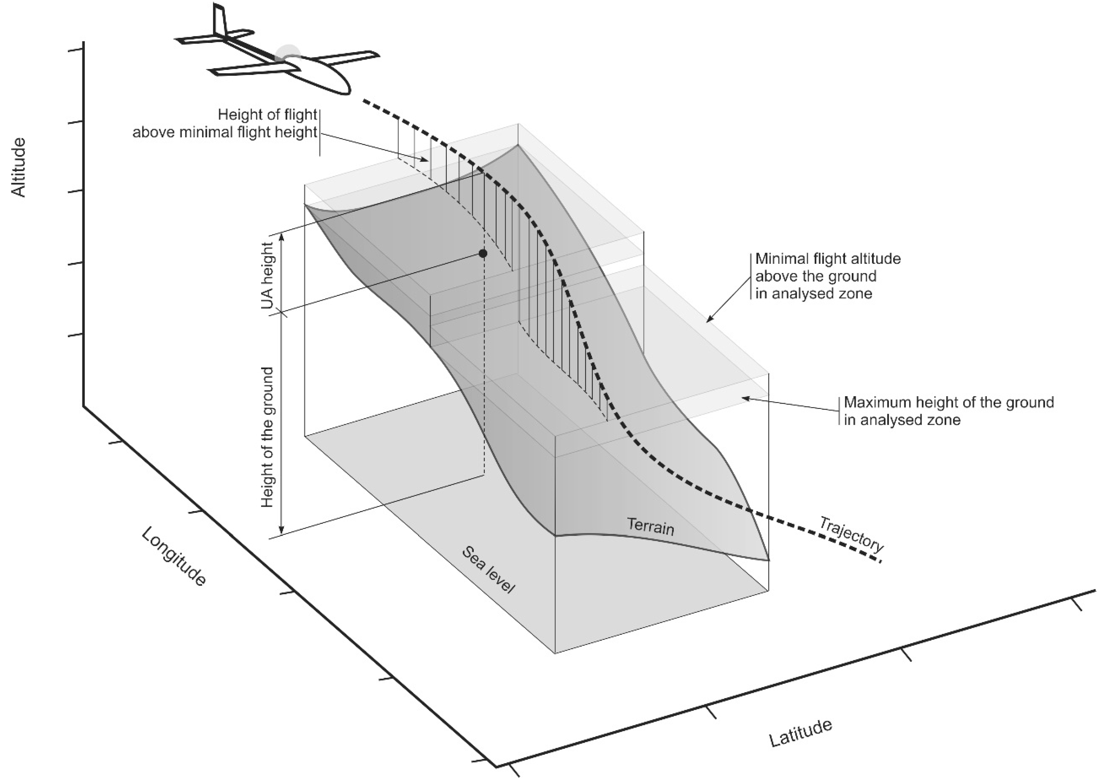
Figure 3. Search for the optimal trajectory required to avoid prohibited zones.

Figure 3. Search for the optimal trajectory required to avoid prohibited zones.

4. Analyzed Case: Total Power Loss of the Power Unit

The situation when a UA’s engine stops working during a flight is very dangerous. First of all, the condition of reaching the airport or landing field will be checked in the flight with maximal lift to drag ratio regarding the necessity to perform the maneuver in the direction of this destination. If the destination is situated within gliding flight range, the optimal trajectory of the approach to this point will be determined with minimal loss of total energy. It will also be checked to ensure that exploitation limitations of the UA are not exceeded. The initial value of the total energy is determined on the basis of:

$$e_{c0}=h_0+\frac{V_0^2}{2g}$$

(12)

The flight of the UA with continuous energy loss is possible up to the moment when its value does not reach final energy defined by the touchdown conditions (height and speed):

$$e_{cf}=h_f+\frac{V_f^2}{2g}$$

(13)

The variation task in this case is formulated as follows: to establish such a control of the UA which, for the given final conditions: x_f, y_f, z_f, γ_f, ψ_f, e_cf and initial conditions z₀, V₀, γ₀, ψ₀, will guarantee maximal distance covered by the aircraft to the final point:

$$r=\sqrt{{\left(x_0-x_f\right)}^2+{\left(y_0-y_f\right)}^2}$$

(14)

Initial values of the coordinates x₀ and y₀ are also determined. However, in this task they are subject to variation. The three-dimensional motion of the aircraft is described by Equation (7) for the thrust equaling zero and a constant weight of the aircraft. That is why the aircraft is controlled by only two parameters: coefficient of load n_z and roll angle φ. Symmetrical coefficients of the load are determined on the basis of:

$$n_Z=\frac{C_L\text{ρ}S{V}^2}{2mg},n_X=\frac{C_D\text{ρ}S{V}^2}{2mg}$$

(15)

The set of Equation (7), written regarding τ [16], acquires the following form:

$$\begin{array}{l}{V}^{\prime }=\frac{g}{\text{λ}}\left(n_X-\sin \text{γ}\right),{\text{γ}}^{\prime }=\frac{g}{\text{λ}V}\left(n_Z\cos \text{φ}-\cos \text{γ}\right),{\psi }^{\prime }=\frac{g}{V\text{λ}\cos \text{γ}}{n}_Z\sin \text{φ}\\ x^{\prime }=\frac{V}{\text{λ}}\cos \text{γ}\cos \text{ψ},y^{\prime }=\frac{V}{\text{λ}}\cos \text{γ}\sin \text{ψ},z^{\prime }=\frac{V}{\text{λ}}\sin \text{γ},t^{\prime }=\frac{1}{\text{λ}}\end{array}$$

(16)

The equation describing the change of total energy of the aircraft completes Equation (16):

$$e_c\left(\text{τ}\right)=e_{c0}-e_{cf}-{\displaystyle \underset{0}{\overset{\tau }{\int }}d{e}_c}$$

(17)

From the second and the third equations of Equation (16), the controlling functions tgφ and n_z are determined. From the fourth, fifth, and sixth equation values, λ, sinγ and tgψ, are determined. The derivatives γ' and ψ' are determined on the basis of:

$${\text{γ}}^{\prime }=\frac{z^{″}\left({x^{\prime }}^2+{y^{\prime }}^2\right)-z^{\prime }\left(x^{\prime }{x}^{″}+y^{\prime }{y}^{″}+z^{\prime }{z}^{″}\right)}{{\left({x^{\prime }}^2+{y^{\prime }}^2+{z^{\prime }}^2\right)}^{\frac{3}{2}}\cos \text{γ}}$$

(18)

$${\text{ψ}}^{\prime }=\frac{{\cos }^2\text{ψ}\left(x^{\prime }{y}^{″}-y^{\prime }{x}^{″}\right)}{{x^{\prime }}^2}$$

(19)

Thus, only the first and the seventh equations will be integrated in Equation (16). In the course of calculations in the right directions of Equations (18) and Equation (19) the values V(τ), x'(τ), y'(τ), z'(τ), x''(τ), y''(τ), z''(τ) are substituted. The speed V(τ) is obtained on basis of integrating the first equation, and the rest of values are determined on the basis of formulas for the support functions x(τ), y(τ), z(τ). Thus, to solve the task of optimization of 3D flight trajectory of an aircraft with non-operated engines, it is necessary to use three approximating polynomials x(τ), y(τ), z(τ), which define the trajectory of motion with the given initial and final conditions.

5. Results and Discussion

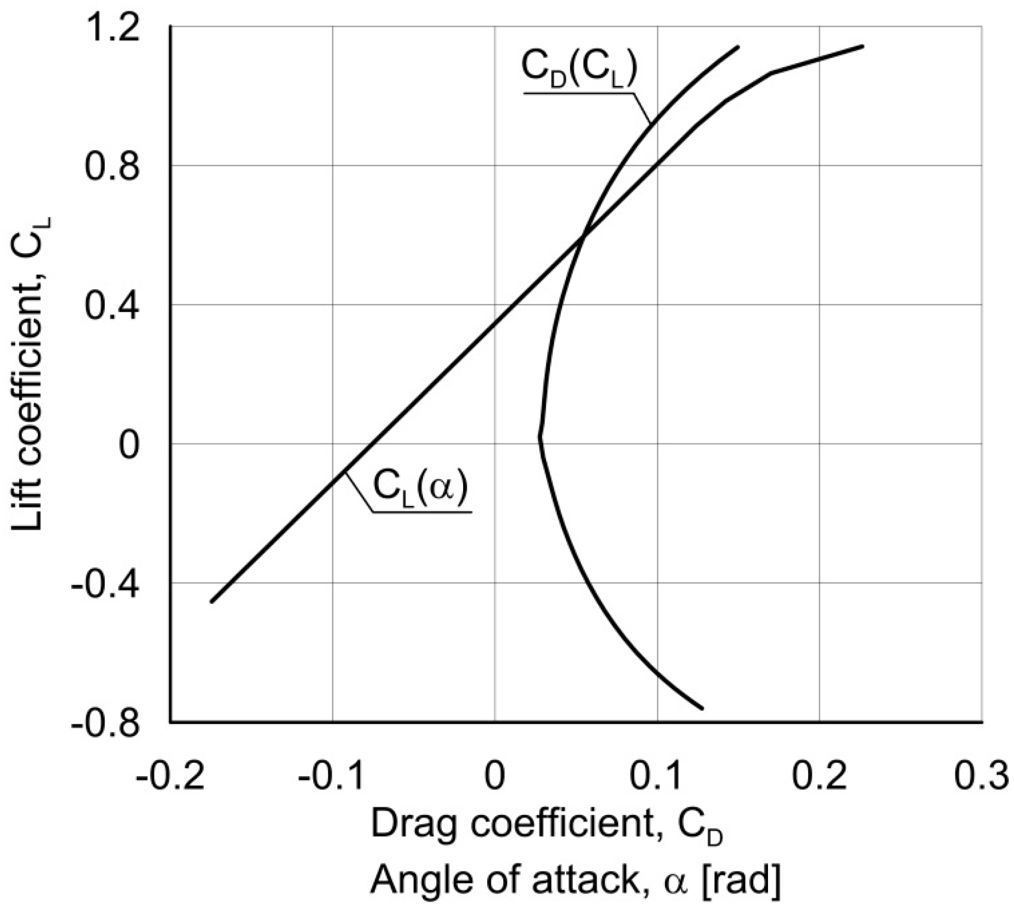
The calculations were carried out for an unmanned vehicle, the DEMON–1, designed at Rzeszow University of Technology (Poland). The main technical characteristics of the DEMON-1 are presented in Table 1. Figure 4 presents the aerodynamic characteristics for the DEMON–1. It was assumed that a distress event, i.e., loss of engine power, appears during a normal flight at a height of 1000 m and at a speed of 35 m/s. The UA flies above the Tyczyn zone near Rzeszow, at a heading of 90°. After loss of engine power, the UA has to reach the UA runway at Boguchwala UAS Airport in gliding flight, avoiding Rzeszow city. At the final position, the aircraft should have at least 50 m of height of flight above the touchdown zone of the UAS runway.

Table 1. General characteristics of DEMON–1.

Parameter	Value	Unit
Length	1.80	m
Wingspan	2.53	m
Wing area	0.86	m2
Gross weight	9.69	kg
Maximum speed	35.65	m/s
Cruise speed	29.40	m/s
Stall speed	12.67	m/s
Rate of climb	4.30	m/s

Table 1. General characteristics of DEMON–1.

Parameter	Value	Unit
Length	1.80	m
Wingspan	2.53	m
Wing area	0.86	m2
Gross weight	9.69	kg
Maximum speed	35.65	m/s
Cruise speed	29.40	m/s
Stall speed	12.67	m/s
Rate of climb	4.30	m/s

Figure 4. Lift coefficient vs. angle of attack and drag polar for the DEMON–1.

Figure 4. Lift coefficient vs. angle of attack and drag polar for the DEMON–1.

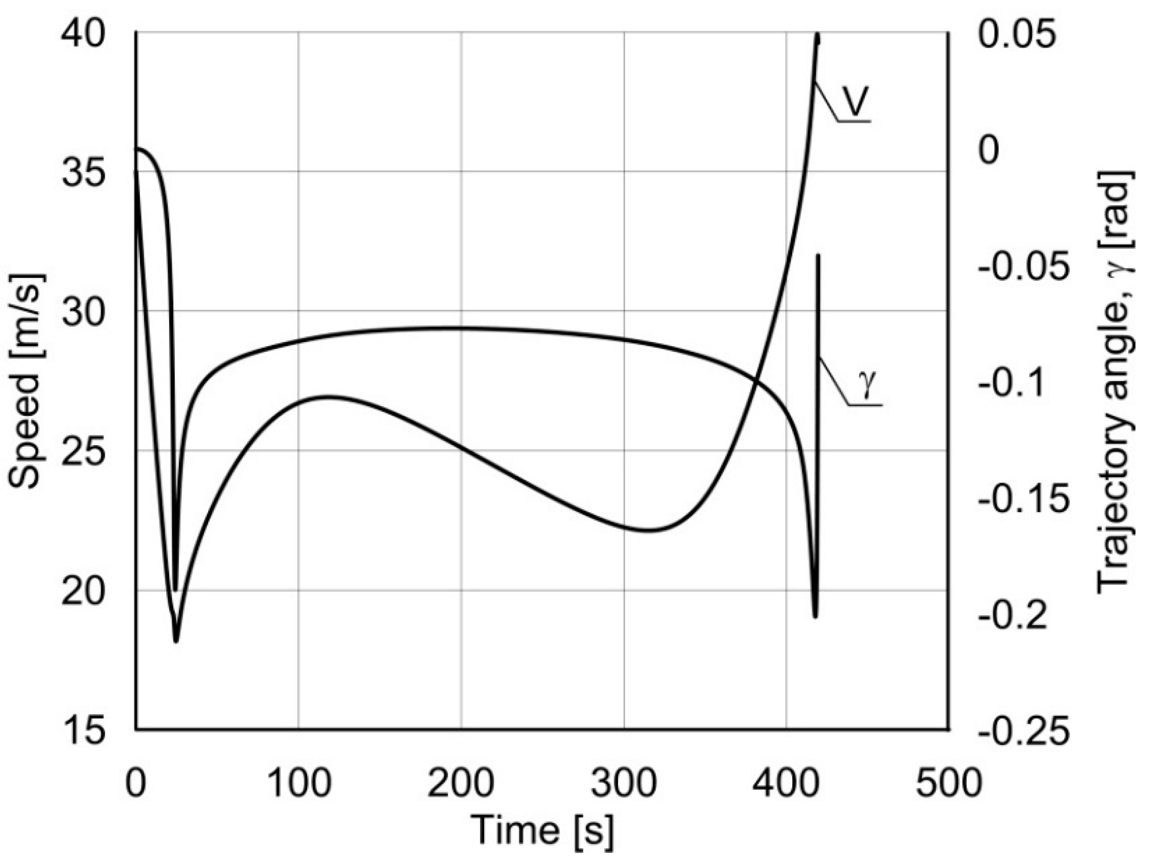
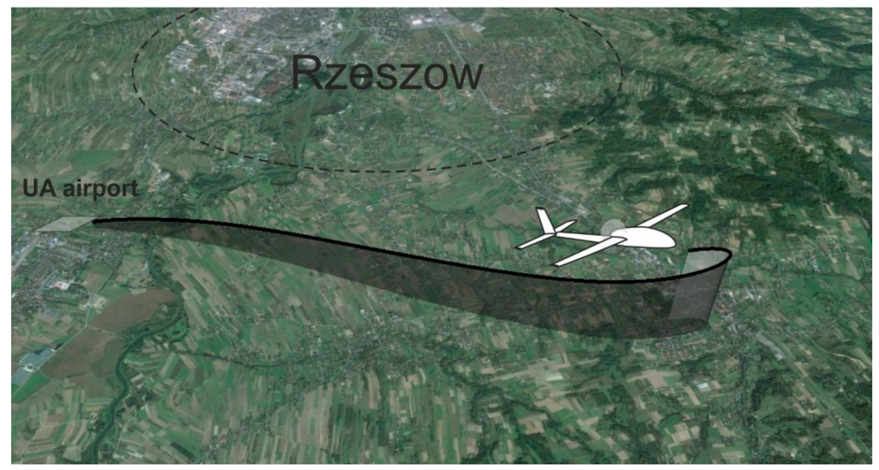
Figure 5 shows the changes of optimal lift and drag coefficients. High lift coefficient, close to maximum value, occurs at the beginning is caused by the sudden maneuver. Figure 6 presents the changes of optimal speed of the UA during flight and changes of trajectory angle. The high decrease of flight speed at the beginning is also caused by the sudden maneuver. The greater change of trajectory angle at the beginning of the gliding phase is caused by the possibility of gliding condition determination. Figure 7 presents the situation map with the shown prohibited area of Rzeszow.

Figure 5. Optimal change of the lift and drag coefficient.

Figure 5. Optimal change of the lift and drag coefficient.

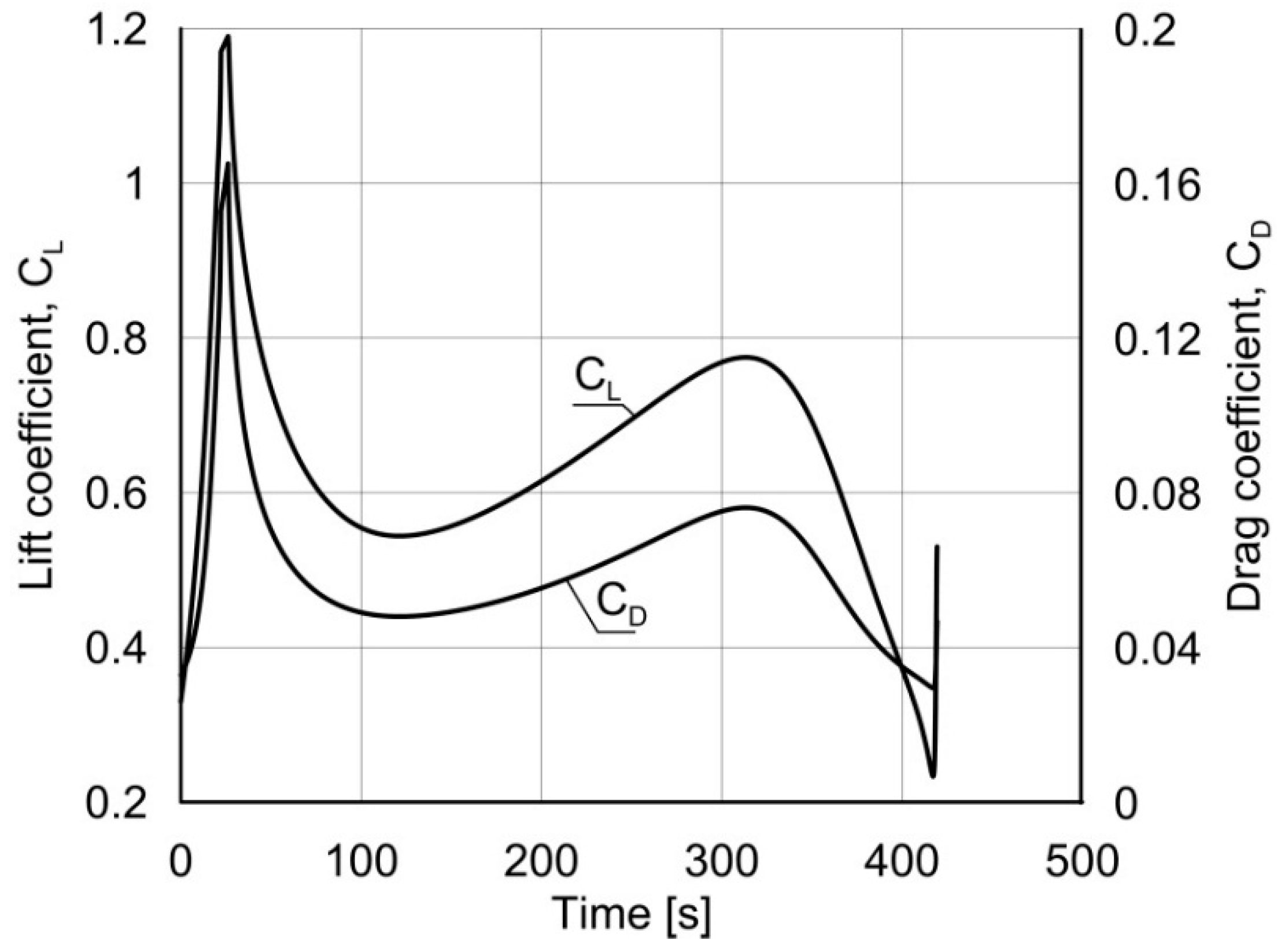
Figure 6. Optimal change of the speed and trajectory angle.

Figure 6. Optimal change of the speed and trajectory angle.

Figure 7. 3D form of the optimal trajectory with the high population area of Rzeszow as the prohibited zone.

Figure 7. 3D form of the optimal trajectory with the high population area of Rzeszow as the prohibited zone.

6. Conclusions

Contemporary UAS have to be designed considering the established parameters of the flight and performance characteristics, which have a direct connection to flight operating safety. Flight operating safety of UA should be understood as a level of adjustment of the system of aircraft behavior, co-existing objects, and the environment when performing a flight plan. Flight operating safety and the effectiveness of using UA are the two basic requirements concerning UAS.

When performing the flight, flight safety is endangered by particular situations that necessitate a change in the regular operation of the UA. Dangerous situations or emergencies are frequently connected with the necessity to change the plan, profile, and parameters of the flight.

The aim of this work was to present the methods used to determine a UA’s flight profile after a dangerous situation or emergency occurs. The analysis was limited to the possibility of an engine system emergency and further flight, continuing along the trajectory of which the shape depends on the type of the emergency. Three possible scenarios in which the emergency takes place were examined:

-

it does not influence the performance of the engine system, however, it limits the time for the UA to get to the destination,

-

it causes a partial loss of performance (power) of the engine system, which necessitates performing a horizontal flight or a flight with a small altitude loss,

-

it causes complete power loss, which necessitates performing a gliding flight only.

The suggested method also enables the determination of the optimal flying trajectory from the territory of a special protection zone (for example large populated areas) in the case of an emergency that disables continuation of the performed task.

The task of this work was to determine the flight parameters of an UA performing the flight to an UA airport or a landing field in the aspect of the minimal value of the assumed functional depending on the analyzed scenario. The method used in this work allows, in a simplified way, a solution to a variation task using the Ritz-Galerkin method, consisting of an approximate solution of the boundary value problem to determine the optimal flight path. The choice of the method was dictated by the fact that it was relatively simple and, at the first step of optimization, it gives a preliminary approximation of the suboptimal path. The UA can start the flight according to the initially determined path of which the shape is corrected through further steps of optimization. Such an approach minimizes the time required to make a decision in an emergency situation. The calculated method can become an element of on-board systems supporting a UAS flight control.

References

- Abdallah, L.; Haddou, M.; Khardi, S. Optimization of operational aircraft parameters reducing noise emission. Appl. Math. Sci. 2010, 4, 515–535. [Google Scholar]
- Khan, S. Flight trajectories optimization. In Proceedings of the ICAS 2002 Congress, Toronto, ON, Canada, 8–13 September 2002.
- Khardi, S. Aircraft flight path optimization, the Hamilton–Jacobi–Bellman considerations. Appl. Math. Sci. 2012, 6, 1221–1249. [Google Scholar]
- Prats, X.; Puig, V.; Quevedo, J.; Nejjari, F. Optimal departure aircraft trajectories minimising population annoyance. In Proceedings of the 3rd International Conference on Research in Air Transportation (ICRAT), Fairfax, VA, USA, 1–4 June 2008.
- Prats, X.; Quevedo, J.; Puig, V. Trajectory management for aircraft noise mitigation. In Proceedings of the ENRI International Workshop on ATM/CNS, Tokyo, Japan, 5–6 March 2009.
- Wijnen, R.A.A.; Visser, H.G. Optimal departure trajectories with respect to sleep disturbance. In Proceedings of the 7th AIAA/CEAS Aeroacoustics Conference, Maastricht, The Netherlands, 28–30 May 2001.
- Bellman, R. The Theory of Dynamic Programing; The Rand Corporation: Santa Monica, CA, USA, 1954. [Google Scholar]
- Pontryagin, L.; Boltyansky, V.; Gamkrelidze, V.; Mischenko, E. Mathematical Theory of Optimal Processes; Wiley-Interscience: New York, NY, USA, 1962. [Google Scholar]
- Taranienko, W.T.; Momdzi, W.G. Simple Variational Method in Boundary Value Problems of Flight Dynamics; Maszinostrojenije: Moscow, Russia, 1986. [Google Scholar]
- Etkin, B.; Reid, L.D. Dynamics of Flight, 3rd ed.; John Willey and Sons: New York, NY, USA, 1996. [Google Scholar]
- Filippone, A. Flight Performance of Fixed and Rotary Wing Aircraft; Elsevier: Burlington, UK, 2006. [Google Scholar]
- Gudmundsson, S. General Aviation Aircraft Design: Applied Methods and Procedures; Elsevier: Oxford, UK, 2013. [Google Scholar]
- Raymer, D.P. Aircraft Design: A Conceptual Approach, 15th ed.; AIAA Education Series: Los Angeles, California, VA, USA, 2012. [Google Scholar]
- Roskam, J. Airplane Design Part V: Component Weight Estimation; DARcorporation: Ottawa, KS, USA, 1985. [Google Scholar]
- Roskam, J. Airplane Design Part VI: Preliminary Calculation of Aerodynamic, Thrust and Power Characteristics; DARcorporation: Ottawa, KS, USA, 1987. [Google Scholar]
- Torenbeek, E. Synthesis of Subsonic Airplane Design; Delft University Press: Rotterdam, The Netherlands, 1976. [Google Scholar]
© 2015 by the authors; licensee MDPI, Basel, Switzerland. This article is an open access article distributed under the terms and conditions of the Creative Commons Attribution license (http://creativecommons.org/licenses/by/4.0/).
Share and Cite
MDPI and ACS Style
Majka, A. Trajectory Management of the Unmanned Aircraft System (UAS) in Emergency Situation. Aerospace 2015, 2, 222-234. https://doi.org/10.3390/aerospace2020222
AMA Style
Majka A. Trajectory Management of the Unmanned Aircraft System (UAS) in Emergency Situation. Aerospace. 2015; 2(2):222-234. https://doi.org/10.3390/aerospace2020222
Chicago/Turabian StyleMajka, Andrzej. 2015. "Trajectory Management of the Unmanned Aircraft System (UAS) in Emergency Situation" Aerospace 2, no. 2: 222-234. https://doi.org/10.3390/aerospace2020222