Article

Development of Flight Path Planning for Multirotor Aerial Vehicles

1
Department of Electrical Engineering, National Chung Hsing University, Taichung 402, Taiwan
2
Aeronautical System Research Division, Chung Shan Institute of Science and Technology, Taichung 407, Taiwan
*
Author to whom correspondence should be addressed.
Aerospace 2015, 2(2), 171-188; https://doi.org/10.3390/aerospace2020171
Submission received: 21 November 2014 / Revised: 11 March 2015 / Accepted: 24 March 2015 / Published: 27 April 2015
(This article belongs to the Special Issue Unmanned Aerial Systems 2015)

Abstract

:
This study addresses the flight-path planning problem for multirotor aerial vehicles (AVs). We consider the specific features and requirements of real-time flight-path planning and develop a rapidly-exploring random tree (RRT) algorithm to determine a preliminary flight path in three-dimensional space. Since the path obtained by the RRT may not be optimal due to the existence of redundant waypoints. To reduce the cost of energy during AV’s flight, the excessive waypoints need to be refined. We revise the A-star algorithm by adopting the heading of the AV as the key indices while calculating the cost. Bezier curves are finally proposed to smooth the flight path, making it applicable for real-world flight.

Graphical Abstract

1. Introduction

A multirotor unmanned aerial vehicle (UAV) is a rotorcraft with more than two rotors to enhance payload capability and endurance. UAVs are widely used in military strategy, disaster relief, exploration, and topographic reconnaissance. The advantages of UAVs are their higher mobility and lower manufacturing costs compared with conventional aircraft.
There are many methods published in the literature for path planning, such as artificial potential field [1,2], A-star algorithm [3,4], fuzzy logic [5,6], genetic algorithm [7,8] and free floating [9]. Sampling-based algorithms have been developed for solving the path-planning problem in high-dimensional environments [10,11] or complex environments [12,13]. Path planning for UAVs in a three-dimensional (3D) environment, divided into several grids, is presented in [14,15,16]. The asymptotic optimality properties of the standard rapidly-exploring random tree* (RRT*) algorithm is given in [17]. Numerical optimization techniques can be applied to refine the output of RRT* until a locally optimal solution is found [18].
Sampling-based algorithms for path planning, such as the standard RRT [19,20] and probabilistic roadmaps (PRM) [11], can resolve the difficulty of computational complexity in real-time settings. Obstacle detection and avoidance for UAVs has been widely studied with a number of techniques presented [21,22,23]. However, there is still a lack of path planners, especially those tailored to multirotor UAVs in 3D environment.
While RRT algorithms can quickly and efficiently find available flight path candidates and avoid collisions, the outcomes may not be optimal, which might lead to a costly flight path. To address this issue, an A-star algorithm for path refinement is used to improve the preliminary solution of path planning generated by a RRT algorithm. Cost-based motion planners are usually limited to low-dimensional problems in relatively small-sized workspaces. To overcome these limitations, variants and extensions of RRT have been developed, and comparisons with similar algorithms have been conducted previously [24].
The A-star algorithm, a heuristic algorithm is based on the Dijkstra algorithm [25,26] and Best-First Search (BFS) [27]. The Dijkstra algorithm, a graph search algorithm, is used to find the shortest path between the starting and goal nodes. The two algorithms differ in the specifications of their cost indices. The A-star algorithm finds the minimum cost path via the BFS, whereas the Dijkstra algorithm finds the minimum cost path from the starting node to all intermediate nodes.
Bezier curves [28,29] are commonly used in computer graphics and related fields. We extend the concept to the 3D environment suitable for our multirotor UAV flight planning. RRT* is an optimal extension to the standard RRT algorithm [17]. Path planning of UAVs in a 3D environment with the evolutionary algorithm (EA)-based controllers is presented in [30,31,32] using the B-spline curve-based path representation. However, the results ignored obstacle avoidance. To combine the advantages of both approaches, we introduce Bezier curves to reshape the flight path developed in the preliminary design phase by adopting a set of straight-line segments from the A-star algorithm. We define the control nodes of the Bezier curve so that the curve is able to avoid collision with obstacles. We verify the proposed path planning method has been verified via a variety of scenarios. We demonstrate computational efficiency of the proposed approach, which overtakes the integrated RRT and Dijkstra algorithms [28]. Our simulation results validate the proposed method.

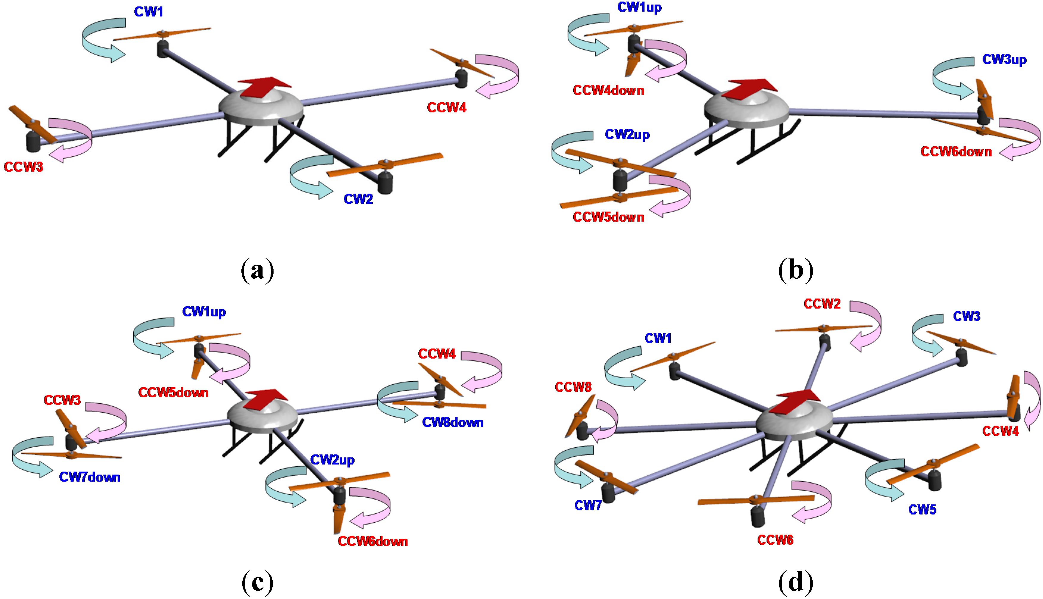
2. Descriptions of Multirotor

Unlike traditional UAVs, a multirotor is a rotorcraft possessing more than two rotors, which can access hard to reach places and, in addition, fly both outdoors and indoors. A helicopter is controlled by changing the angle-of-attack of the propeller, whereas a multirotor is controlled by tuning the speed of different propellers. Multirotors use fixed-pitch blades that means its rotor pitch does not vary as the blades rotate, and control of the vehicle motion is achieved by changing relative speed of each rotor to adjust the thrust and torque produced by each rotor.
Multirotor, usually referred to quadrotor, hexarotor and octorotor, is 4-, 6- and 8-propeller helicopter, respectively. The quadrotor, for instance, has four propellers with hovering capabilities, two pairs of counter-rotating, and fixed-pitch blades located at four corners. Multirotors are capable of generating greater thrust than conventional helicopters and possess better stability during flight. Each propeller produces both thrust and torque about its center of rotation, in the direction opposite to drag. The four propellers are cross-allocated (see Figure 1a); propeller_1 and propeller_3 share the same rotational direction and propeller_2 and propeller_4 share the same rotational direction. The arrow sign in indicates the directional movements of common multirotor UAVs.
Figure 1. Schematic of movement for typical multirotor: (a) quadrotor; (b) hexarotor; (c) octorotor_type1; and (d) octorotor_type2.
Aerospace 02 00171 g001

3. Overview of the Proposed Flight Path Planner

In the proposed flight path planner, we first adopt multi-RRT algorithm to randomly generate potential flight path candidates by generating collision-free waypoints. However, the paths generated are, in general, not optimal due to existence of redundant waypoints; we next propose an improved A-star algorithm to refine the path from the starting node to the goal node. Finally, Bezier curves are incorporated to reshape the flight path for a smoothed flight and to further reduce the flight cost by removing unnecessary waypoints.
A flow chart of the path planning for multirotor UAVs is illustrated in Figure 2. We first specify the start and goal headings of the UAV. Next, the multi-RRT algorithm is applied to construct the available paths. If there is no available candidate, the algorithm reports an error. If at least one qualified path is found, we continue to apply the improved A-star algorithm and Bezier curves to complete simplification and smoothed path.
Figure 2. Flow chart of the proposed path planner.
Aerospace 02 00171 g002

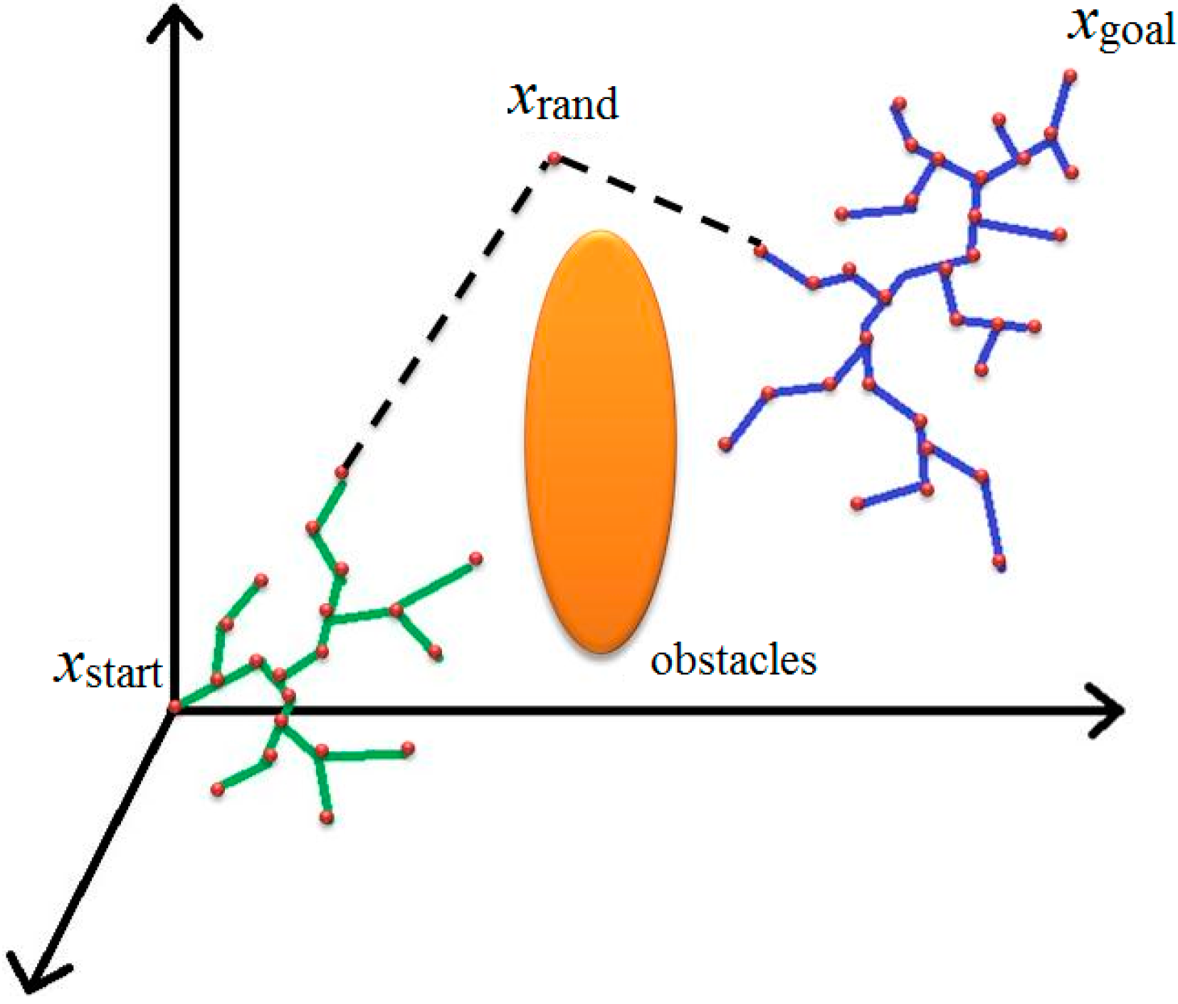
3.1. Rapidly-Exploring Random Tree (RRT)

The basic-RRT algorithm for path planning has been shown to be efficient in high-dimensional environments [11]. However, the paths found are not necessarily optimal. The basic-RRT searches for the path from the starting node to the goal nodes by growing a bunch of random trees in a high-dimensional environment until the goal node becomes a node of the random tree. A tree is grown from the starting node to the goal node by adding a new edge and a new node at each iteration. The basic-RRT algorithm works with three steps:
(1)
Generation of random nodes: pick the random nodes in 3D environment.
(2)
Expansion: pick a random node and then build connection between this node and the nearest node in the random tree.
(3)
Termination condition: join the goal node to the random tree.
The multi-RRT uses two random trees to generate a possible path. The random trees are generated bi-directionally: one is built from xstart and the other is expanded from xgoal. When a linkage connects xnearest and xnew with some obstacles interfered, the multi-RRT algorithm regenerates a new random tree in terms of xrand. When the environment of the path planning is relatively complicated, i.e., the chance of collision between obstacles is relatively high, the convergence rate of the multi-RRT is better than that of the basic-RRT. When a random node connects two random trees, the node yields a feasible path, as shown in Figure 3.
Figure 3. Random node connecting two random trees.
Aerospace 02 00171 g003

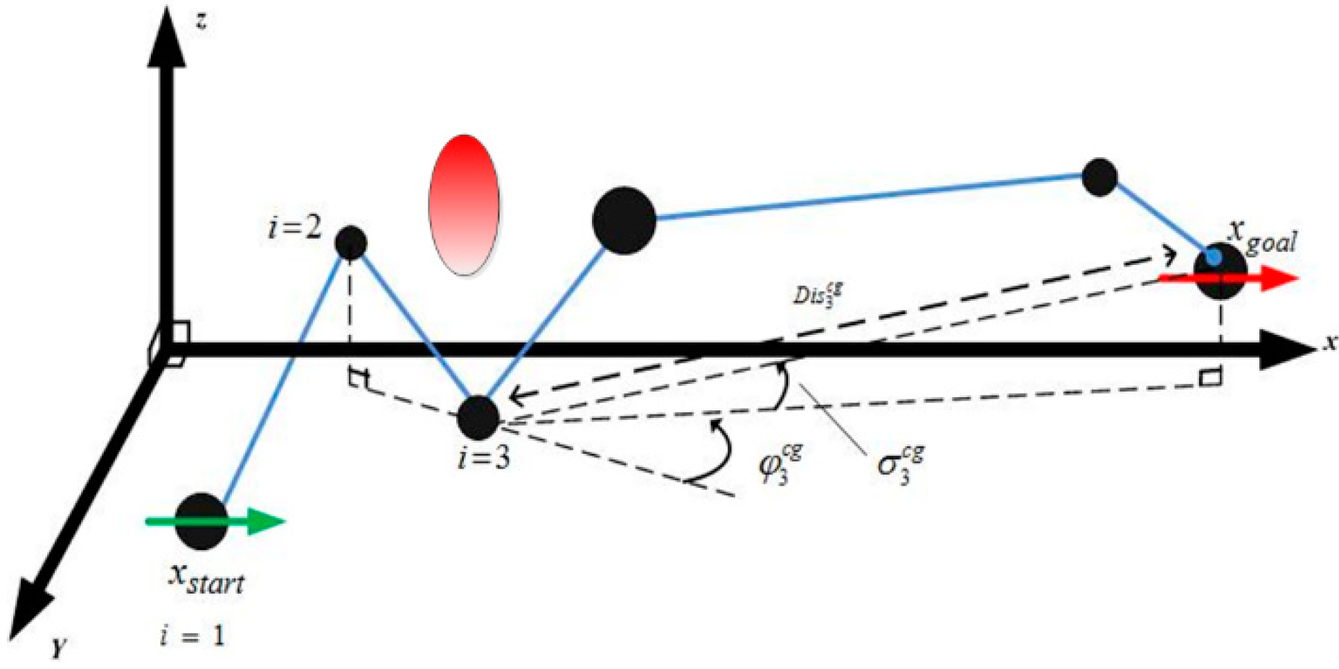
3.2. A-Star Algorithm

The path planning described above ensures efficient and collision-free motion of a multirotor in a 3D environment with unknown static obstacles. This section describes the basic A-star algorithm and how we use it to smooth a path for multirotors.
In general, there will be bifurcations of the flight path when there are obstacles around. Collision free waypoints are generated for an appropriate potential flight path, which is constituted by several line segments. The potential flight paths are next smoothed to avoid sharp flight paths.
The basic A-star algorithm possesses three parts:
(1)
An open list: save all next reachable nodes from the current node.
(2)
A closed list: save already through nodes from the starting node to the current node.
(3)
An evaluation function: determine the order of the expanded nodes; the cost equation at each node of A-star is set as
F i = G i + H i
where the subscript i denotes the ith node in the multi-RRT, Gi is the ith moving cost from the starting node to the current node, Hi is the estimated cost of the ith node from the current node to the goal node, and Fi is the total moving cost from the starting node to the goal node. There are three operational steps:
Step 1
Add the starting node to the open list.
Step 2
Find the lowest Fi on the open list referring to the current node and add the ith to the closed list with the ith node canceled from the open list.
Step 3
Check whether the ith node can reach the adjacent nodes. If the ith node is not on both lists, add it to the open list. If the ith node is on the open list, and the new F is lower than the original F, then the new F refers to the original F; update the last index of the adjacent node as the current node.
Step 4
If the goal node is on the closed list, the path is found. If the goal node is not on the closed list, repeat Step 2. If the open list is empty, there is no available path.
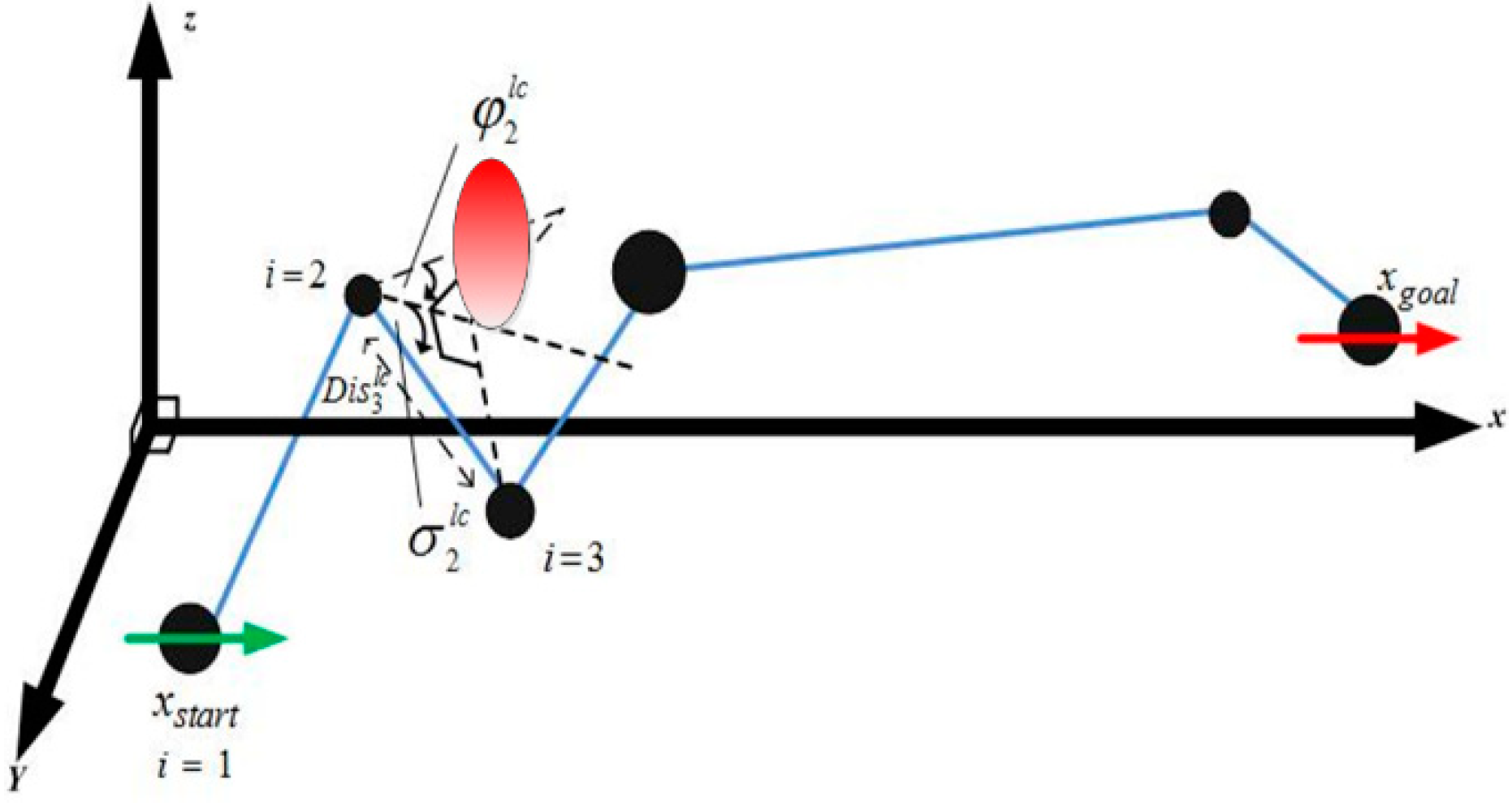
The basic A-star algorithm divides the environment into several grids before conducting path planning and memorizing the indices of via the points. However, this requires a significant amount of memory. Therefore, we propose an improved A-star algorithm instead by considering only the absolute values of the flight path angles, i.e., the moving cost Gi, as follows:
(1)
when the climbing angle σ i 1 l c and the yaw angle φ i 1 l c are less than 90°
G i = D i s i 1 l c × ( 1 + sin σ i 1 l c + sin φ i 1 l c ) + G l
(2)
when σ i 1 l c is greater than 90° and φ i 1 l c is less than 90°
G i = D i s i l c × ( 2 + sin ( σ i 1 l c π 2 ) + sin φ i 1 l c ) + G l
(3)
when σ i 1 l c is less than 90° and φ i 1 l c is greater than 90°
G i = D i s i l c × ( 2 + sin σ i 1 l c + sin ( φ i 1 l c π 2 ) ) + G l
(4)
when σ i 1 l c and φ i 1 l c are greater than 90°
G i = D i s i l c × ( 3 + sin ( σ i 1 l c π 2 ) + sin ( φ i 1 l c π 2 ) ) + G l
The estimated cost Hi is given by
(1)
when σ i c g and φ i c g are less than 90°
H i = D i s i c g × ( 1 + sin σ i c g + sin φ i c g )
(2)
when σ i c g is greater than 90° and φ i c g is less than 90°
H i = D i s i c g × ( 2 + sin ( σ i c g π 2 ) + sin φ i c g )
(3)
when σ i c g is less than 90° and φ i c g is greater than 90°
H i = D i s i c g × ( 2 + sin σ i c g + sin ( φ i c g π 2 ) )
(4)
when σ i c g and φ i c g are greater than 90°
H i = D i s i c g × ( 3 + sin ( σ i c g π 2 ) + sin ( φ i c g π 2 ) )
where the range of i is the total number of multi-RRT nodes, Gl denotes the current node, D i s i c g is the distance from the previous node to the current node, D i s i c g is the distance from the current node to the goal node, φ i 1 l c and φ i c g are, respectively, the yaw angles from the current node to the adjacent node and the yaw angles from the current node to the goal node through the adjacent node of the current node, σ i 1 l c and σ i c g are, respectively, the climbing angles from the current node to the adjacent nodes and the climbing angles from the current node to the goal node through the adjacent node of the current node.

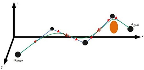
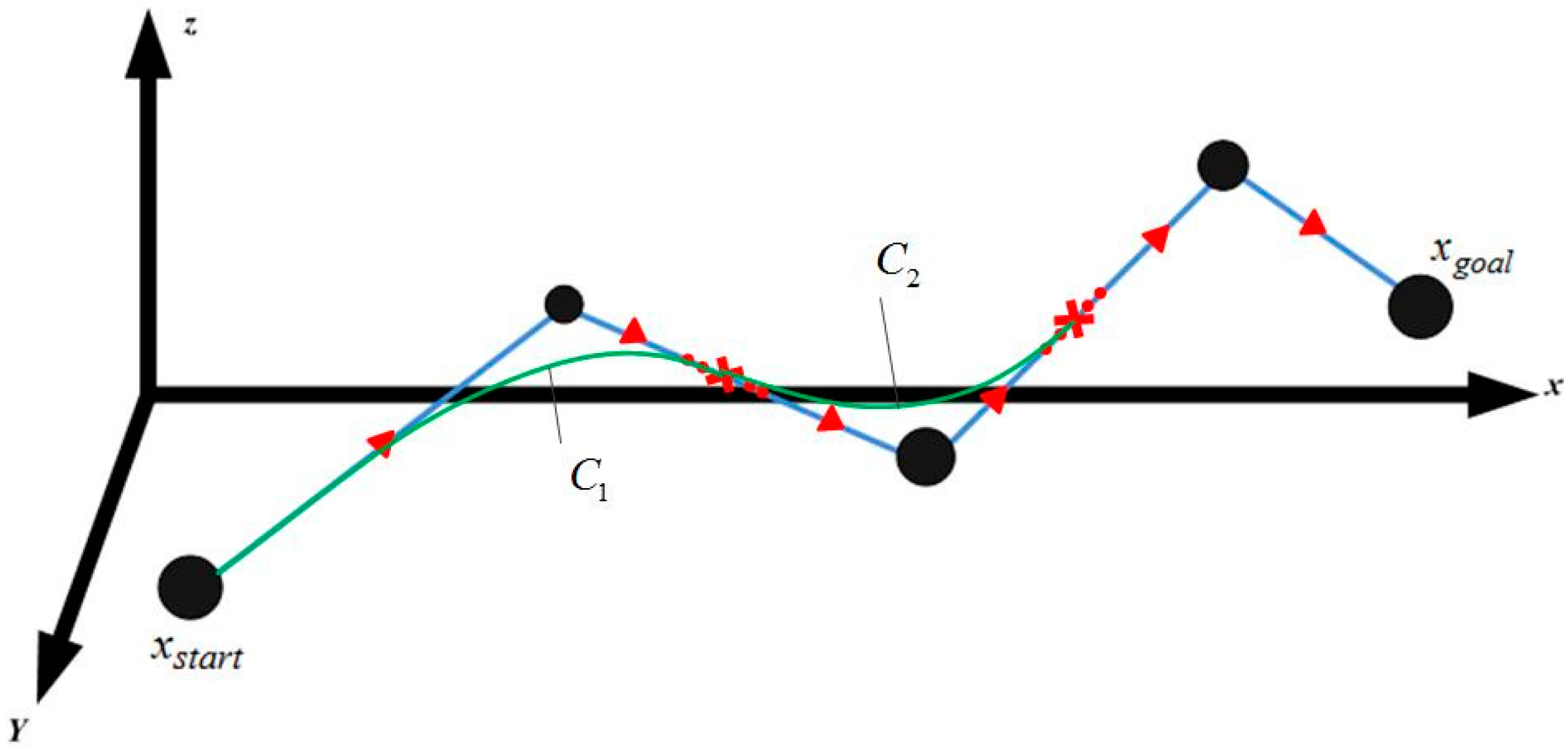
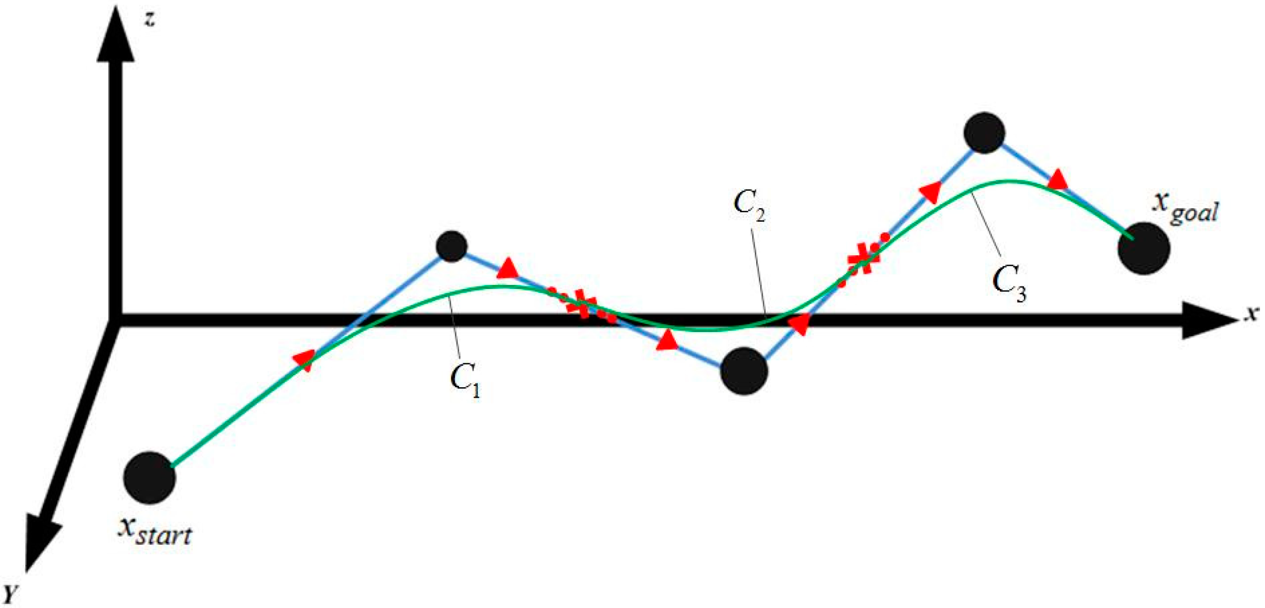
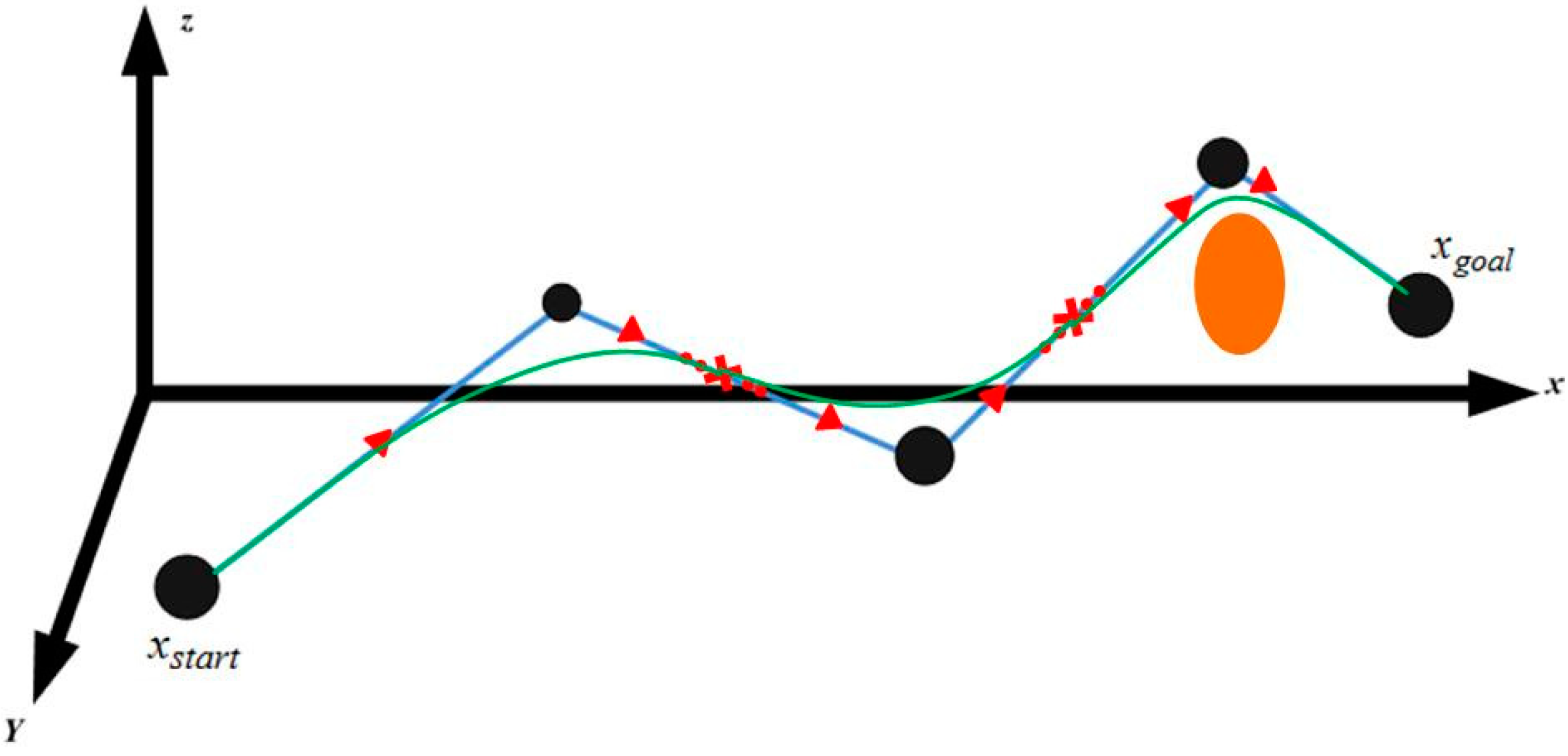
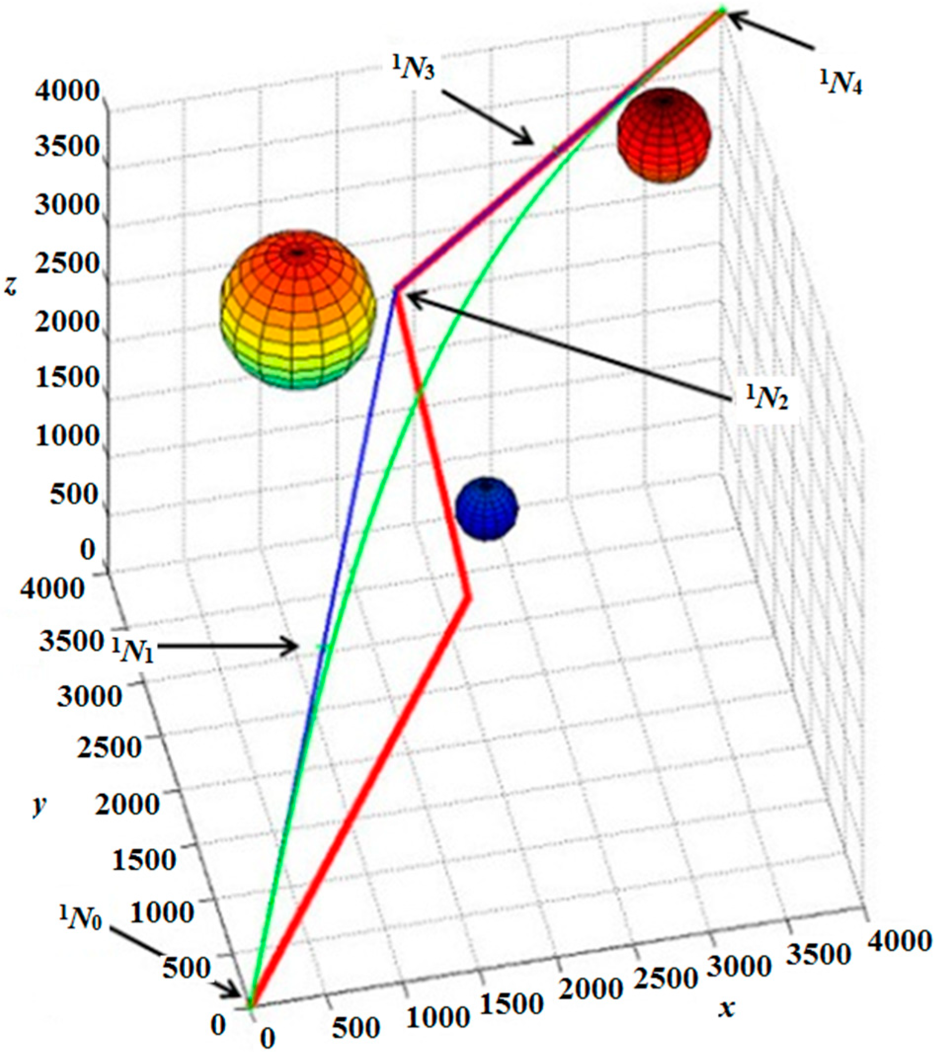
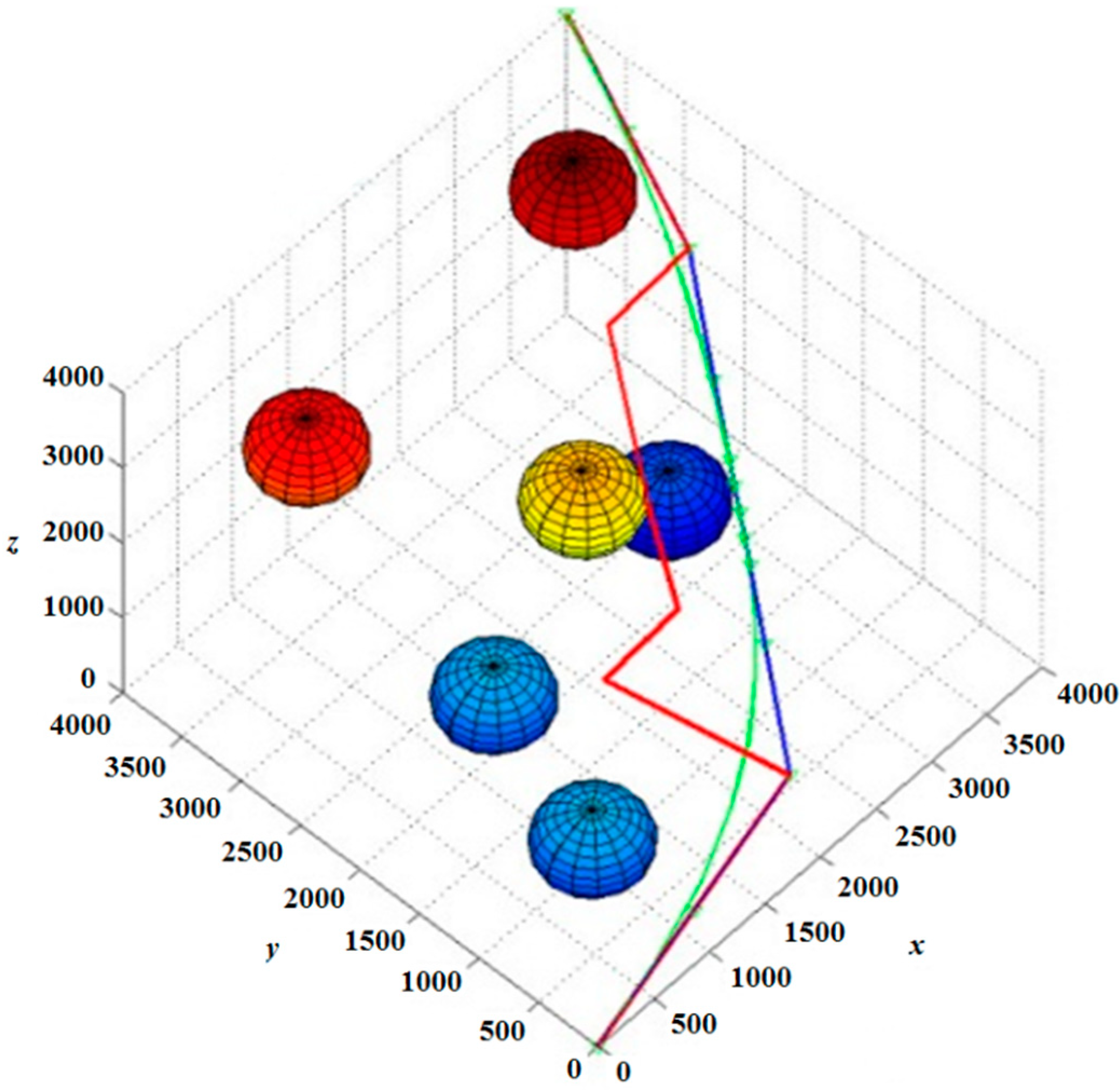
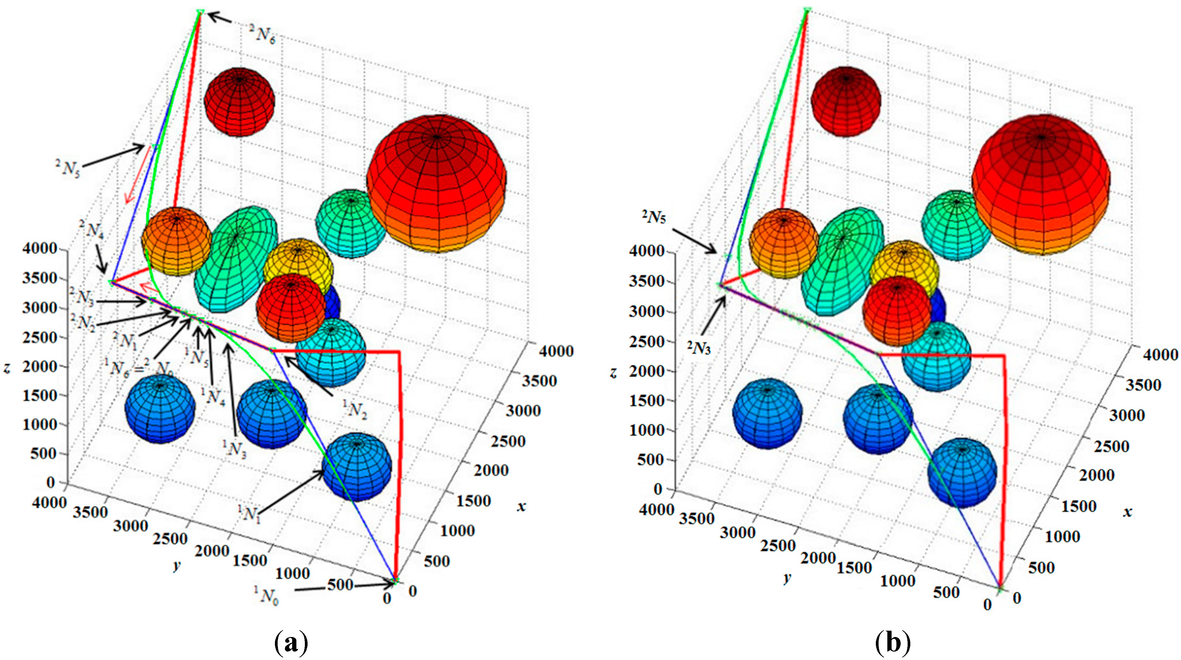
3.3. Flight Path Refinement

Here, we introduce the improved A-star algorithm to resolve the optimality problem. In Figure 4 and Figure 5, the green arrow indicates the start headings of the UAV, the red arrow refers to the goal heading, i denotes the index of the nodes, xstart and xgoal, and the blue lines are the paths generated by the multi-RRT algorithm.
Figure 4. Computing φ 2 l c and σ 2 l c .
Aerospace 02 00171 g004
The climbing angle of UAV is controlled by the angles of pitch and roll. The angle of horizontal rotation is generated by changing the yaw angle. In Figure 4, let i = 2 and compute the yaw angle φ 2 l c , the climbing angle σ 2 l c , and D i s 3 l c , which is the distance between the nodes indexed i = 2,3. Next, substituting φ 2 l c , θ 2 l c (all less than 90°) and D i s 3 l c into Equation (2) obtains the moving cost G3.
Figure 5. Computing φ 3 c g and σ 3 c g .
Aerospace 02 00171 g005
In Figure 5, we compute φ 2 c g , σ 3 c g (all less than 90°) and D i s 3 c g , which are the distances between the third node and xgoal. Next, substituting the three variables into Equation (6) to gives the estimated cost H3. Finally, substituting G3 and H3 into Equation (1), one obtains the total moving cost index F3 repeating the process results in a class of refined flight paths.

3.4. Bezier Curves

We next apply Bezier curves [28] to shorten and smooth the path. To proceed, we define the Bezier curves of degree nk as
C k ( t ) = i = 0 n k B i , n k ( t ) k N i
where k indicates the index of the Bezier curve, k ∈ {1, 2, l, m}, kNi are the control nodes of the Bezier curves, and B i , n k ( t ) are the Bernstein polynomials of degree nk as
B i , n k ( t ) = n k ! i ! ( n k i ) ! t i ( 1 t ) n k i
When two or more Bezier curves need to be joined together, the interconnected points should be continuous, i.e., the first- and the second-order derivatives of two successive Bezier curves should remain the same at the interconnected point. The first-order derivative of Bezier curves is given by
C k ( t ) = i = 0 n 1 B i , n 1 ( t ) k D i
where the first control nodes kDi = n(kNi+1kNi). The second-order derivative of Bezier curves is
C k ( t ) = i = 0 n 2 B i , n 2 ( t ) k E i
where the second control nodes kEi = n(kNi+2 − 2kNi+1 + kNi). The requirement of continuity in the Bezier curves is
C k ( 1 ) = C k + 1 ( 0 )
then
n k ( N n k k N n k 1 k ) = n k + 1 ( N 1 k + 1 N 0 k + 1 )
C ¨ k ( 1 ) = C ¨ k + 1 ( 0 )
and
n k ( n k 1 ) ( N n k k 2 N n k 1 k + N n k 2 k ) = n k + 1 ( n k + 1 1 ) ( N 2 k + 1 2 N 1 k + 1 + 2 N 0 k + 1 )
We denote {A1, A2, l, Am} the waypoints of the improved A-star algorithm. When the waypoint number m = 3, C1 refers to the fourth-order Bezier curve. When the waypoint number m > 3, {C1, l, Cm−2} constitutes the sixth-order Bezier curves and {C2, C3, l, Cm−4, Cm−3} are the eighth-order Bezier curves.
When m = 3, the Bezier curve of C1 section is
(1)
fixed control nodes
1N0 = A1
1N2 = A2
1N4 = A3
(2)
movable nodes
N 1 1 = N 0 1 + α 1 N 0 1 N 2 1
N 3 1 = N 0 1 + ( 1 α 1 ) N 0 1 N 4 1
When m > 3, the Bezier curves of {C1,l, Cm−2} sections are
(1)
fixed control nodes:
1N0 = A1
1N2 = A2
m−2N4 = Am−1
m−2N6 = Am
N 6 1 = N 0 2 + 0.5 N 2 1 N 4 2
N 8 m 3 = N 0 m 2 = N 4 m 3 + 0.5 N 4 m 3 N 4 m 2
(2)
movable control nodes:
N 1 1 = N 0 1 + α 1 N 0 1 N 2 1
N 3 1 = N 0 2 + ( 1 α 1 ) N 0 2 N 4 2
N 3 m 2 = N 0 m 2 + α m 2 N 0 m 2 N 4 m 2
N 5 m 2 = N 4 m 2 ( 1 α m 2 ) N 4 m 2 N 5 m 2
(3)
interconnected nodes:
n 1 ( N n 1 1     N n 1 1 1 ) = n 2 ( N 1 2 N 0 2 )
n 1 ( n 1 1 ) ( N n 1 1     2 N n 1 1 1 + N n 1 2 1 ) = n 2 ( n 2 1 ) ( N 2 2 2 N 1 2 + N 0 2 )
n m 3 ( N n m 3 m 3     N n m 3 1 m 3 ) = n m 2 ( N 1 m 2 N 0 m 2 )
n m 3 ( n m 3 1 ) ( N n m 3 m 3     2 N n m 3 1 m 3 + N n m 2 m 3 ) = n m 2 ( n m 2 1 ) ( N 2 m 2 2 N 1 m 2 + N 0 m 2 )
When m > 3, the Bezier curves {C2, C3, l, Cm−4, Cm−3} are
(1)
fixed control nodes:
N 4 i 1 = A i ,     i { 3 , 4 , l , m 2 }
N 8 i = N 0 i + 1 = N 4 i + 0.5 N 4 i + 1 i N 4 ,     i { 2 , 3 , l , m 3 }
(2)
movable control nodes:
N 3 j = N 0 j + α j N 0 j N 4 j ,     j { 2 , 3 , l , m 3 }
N 5 j = N 0 j + 1 + ( 1 α j ) N 0 j + 1 N 4 j + 1 ,     j { 2 , 3 , l , m 3 }
(3)
interconnected nodes:
n r ( N n r r     N n r 1 r ) = n r + 1 ( N 1 r + 1 N 0 r + 1 ) ,     r { 1 , 2 , l , m 3 }
n r ( n r 1 ) ( N n r r     2 N n r 1 r + N n r 2 r ) = n r + 1 ( n r + 1 1 ) ( N 2 r + 1 2 N 1 r + 1 + N 0 r + 1 ) ,     r { 1 , 2 , l , m 3 }
where αj ∈ {0, 1} is the weighting factor; in general, the initial weighting factor is set to be 0.5. Selection of the weighting factor depends on the relationship of the movable control nodes between the fixed control and interconnected nodes. Taking Figure 6, Figure 7, Figure 8 and Figure 9 as examples, we assume that the improved A-star algorithm generates the blue path and that {A1, A2, l, A5} are the waypoints of the path. Before applying the Bezier curves, it is necessary to determine control nodes, as indicated in Figure 6. Figure 7, Figure 8 and Figure 9 illustrate the sixth-order, eight-order and sixth-order Bezier curves constituted by the sets of control nodes {1N0, 1N1, l, 1N6}, {2N0, 2N1, l, 2N8} and {3N0, 3N1, l, 3N6}, respectively.
Figure 6. Positions of the control nodes.
Aerospace 02 00171 g006
Figure 7. Result of the sixth-order Bezier curve C1 constituted by the nodes {1N0, 1N1, l, 1N6}.
Aerospace 02 00171 g007
Figure 8. Result of the eighth-order Bezier curve C2 constituted by the nodes {2N0, 2N1, l, 2N8}.
Aerospace 02 00171 g008
Figure 9. Result of the sixth-order Bezier curve C3 constituted by the nodes {3N0, 3N1, l, 3N6}.
Aerospace 02 00171 g009
Recall that the resulting path determined above could be interfered with obstacles, we select control nodes of the Bezier curves so that the modified curves could avoid the obstacles. For example, in Figure 10, the curve C3 collides with the orange-colored obstacle. One may consider adding movable control nodes between the fixed control nodes and the interconnected nodes of the obstacle and change the weighting factor α3 to shift the control nodes, 3N3 and 3N5. This leads C3 away from the obstacle, see Figure 11.
Figure 10. C3 collides with the obstacle.
Aerospace 02 00171 g010
Figure 11. C3 avoids the obstacle.
Aerospace 02 00171 g011

4. Simulation Results

4.1. Path Planning in 3D Environment

To evaluate the performance of the proposed multirotor UAV path-planning algorithm, we consider three scenarios.

4.1.1. Scenario 1

The flight path is generated by the multi-RRT algorithm with four waypoints (the red line in Figure 12). We adopt the improved A-star algorithm in blue line to refine the path moving cost. After conducting the improved A-star algorithm, the number of waypoints decreases from four to three (see Table 1), i.e., m = 3. Incorporating Equations (18)–(22) yields a Bezier curve illustrated as the green line in Figure 12.
Figure 12. Results of path planning via the multi-RRT and improved A-star algorithms and the finalized path after introducing Bezier curves in Case 1 (unit: m).
Aerospace 02 00171 g012
Table 1. Waypoints of the paths generated by the multi-RRT (rapidly-exploring random tree) and improved A-star algorithms.
Path Planning Waypoints of Case 1
Multi-RRT Waypoints (m)Improved A-Star Waypoints (m)
(0, 0, 0)(0, 0, 0)
(1954.4, 2314.1, 949.1)
(1835.4, 3852.4, 2187.2)(1835.4, 3852.4, 2187.2)
(4000, 4000, 4000)(4000, 4000, 4000)

4.1.2. Scenario 2

After fulfilling the improved A-star algorithm, the number of waypoints of the path decreases from eight to four (see Table 2). Combining Equations (18)–(22) yields the Bezier curves, as illustrated in Figure 13.
Table 2. Waypoints of the paths generated by the multi-RRT and improved A-star algorithms.
Path Planning Waypoints of Case 2
Multi-RRT WaypointsImproved A-Star Waypoints
(0, 0, 0)(0, 0, 0)
(1912.0, 168.0, 998.2)(1912.0, 168.0, 998.2)
(896.3, 780.5, 2840.6)
(1457.6, 685.9, 3181.4)
(1970.7, 1418.5, 3100.2)
(2546.3, 2283.6, 3708.4)(2546.3, 2283.6, 3708.4)
(3647.9, 2638.7, 2909.5)(3647.9, 2638.7, 2909.5)
(4000, 4000, 4000)(4000, 4000, 4000)
Figure 13. Results of path planning via the multi-RRT and improved A-star algorithms and the finalized path after introducing Bezier curves in Case 2 (unit: m).
Aerospace 02 00171 g013

4.1.3. Scenario 3

The resulting path retains four waypoints, i.e., m = 5. Using Equations (23)–(42) generates the corresponding. Note, however, that the flight path may still collide the obstacles as shown in Figure 14a and Table 3. We adjust the movable nodes so that the flight path can avoid the obstacle. Here, the weighting factor α2 in Equations (31) and (32) is increased gradually so that the curves will bypass the obstacles. The satisfactory result with α2 = 0.9 is finally reached (Figure 14b).
Figure 14. Path planning result of the multi-RRT and A-star algorithms and the finalized path after introducing Bezier curves in Case 3 (unit: m). (a) The finalized path collides with obstacles; (b) The finalized path avoids the obstacles.
Aerospace 02 00171 g014
Table 3. Waypoints of the paths generated by the multi-RRT and improved A-star algorithms.
Path Planning Waypoints of Case 3
Multi-RRT Waypoints (m)Improved A-Star Waypoints (m)
(0, 0, 0)(0, 0, 0)
(728.6, 167.3, 427.8)(728.6, 167.3, 427.8)
(2047.3, 330.4, 2878.3)(2047.3, 330.4, 2878.3)
(1646.4, 2410.6, 3002.1)
(2020.5, 3962.2, 3558.8)(2020.5, 3962.2, 3558.8)
(3291.3, 3888.5, 2807.2)
(4000, 4000, 4000)(4000, 4000, 4000)

4.2. Comparison of Performance

In [28], the authors adopted an integrated RRT and Dijkstra algorithms to characterize the flight path for UAVs. Our study, instead, uses the multi-RRT and improved A-star algorithms. We have recorded computation time under the same scenario for performance comparison. The PC equipped with CPU i7 3.4 GHz and RAM 3 GB was adopted. Note that the comparison did not include the part of the construction of Bezier curves, which relies on extra tunings of the weighting factor α. The integrated RRT and Dijkstra algorithms consumed 12.804 s, as shown in Figure 15a, and the integrated multi-RRT and improved A-star algorithms used 0.225 s, see Figure 15b.
Figure 15. Flight paths generated by different algorithms under the same scenario: (a) RRT (red-dotted line) and Dijkstra algorithms (blue line); (b) integrated multi-RRT (red line) and improved A-star algorithms (blue line) (unit: m); and (c) multi-RRT (red line) and improved A-star (blue line) and Bezier curving refinement (unit: m).
Aerospace 02 00171 g015
Concerning about the computational efficiency, Figure 15c shows the smoothed fight path, which took extra time of 0.39 s for each try of α while incorporating Bezier curves for smoothing. We have considered three tries (α = 2, 1, 0.5). This figure shows the result with α = 0.5. Table 4 summarizes the required computation time.
Table 4. Comparison of computational efficiency.
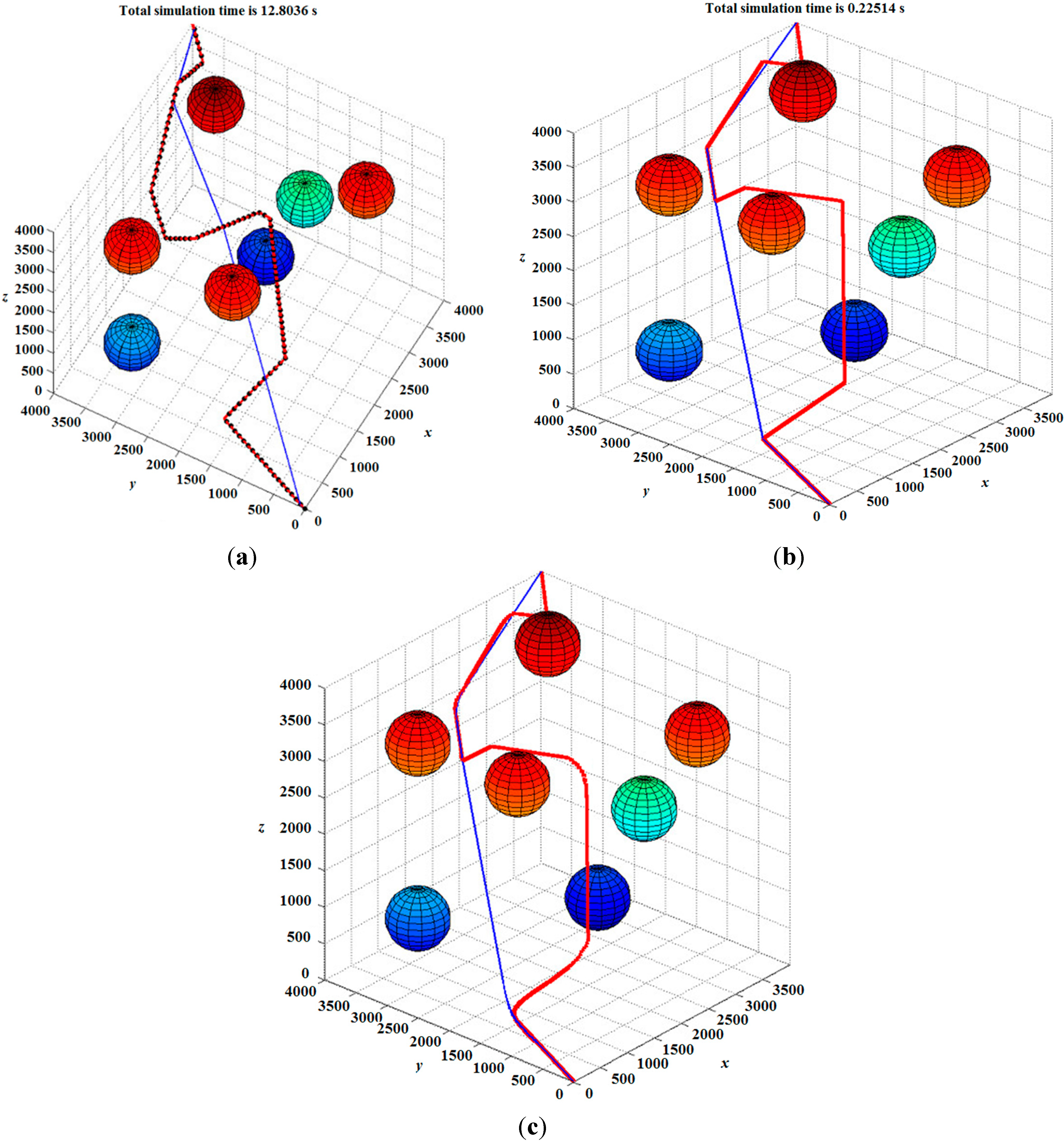
Results of Comparison of Computation Time
AlgorithmsRRT + DijkstraMulti-RRT + Improved A-StarMulti-RRT + Improved A-Star + Bezier’s Curving Refinement
Total time (s)12.8040.2251.395

5. Conclusions

This study proposed a novel path planning method for multirotor UAVs in a 3D environment. To account for real-time navigation, a multi-RRT algorithm was introduced to characterize the preliminary flight paths in an efficient manner. The proposed improved A-star algorithm tailored for multirotor UAVs was incorporated to mitigate flight path costs by reducing the number of waypoints. As for flight path smoothing, control nodes of the Bezier curves were determined to refine the paths. A variety of scenarios, from single to multiple obstacles, were numerically simulated and evaluated. The results showed that the combined use of the proposed improved A-star algorithm and the Bezier curves produced smooth flight paths with less cost while remaining computational efficiency.

Author Contributions

Yi-Ju Tsai and Chia-Sung Lee conducted the numerical simulation. Chun-Liang Lin and Yi-Ju Tsai developed the computational algorithms. Chun-Liang Lin responded the review comments. Ching-Huei Huang helped writing the manuscript.

Conflicts of Interest

The authors declare no conflict of interest.

References

  1. Malaek, S.M.; Kosari, A.R. Dynamic based cost functions for TF/TA flights. IEEE Trans. Aerosp. Electron. Syst. 2012, 48, 44–63. [Google Scholar] [CrossRef]
  2. Guldner, J.; Utlun, V.I. Sliding mode control for gradient tracking and robot navigation using artificial potential fields. IEEE Trans. Robot. Autom. 1995, 11, 247–254. [Google Scholar]
  3. Malaek, S.M.; Kosari, A.R. Novel minimum time trajectory planning in terrain following flights. IEEE Trans. Aerosp. Electron. Syst. 2007, 43, 2–12. [Google Scholar] [CrossRef]
  4. Bellman, R. Dynamic Programming; Princeton University Press: Princeton, NJ, USA, 1957. [Google Scholar]
  5. Kurnaz, S.; Cetin, O.; Kaynak, O. Fuzzy logic based approach to design of flight control and navigation tasks for autonomous unmanned aerial vehicles. J. Intell. Robot. Syst. 2009, 54, 229–244. [Google Scholar] [CrossRef]
  6. Francesco, B.; Lorenzo, P.; Mario, I. Waypoint-based fuzzy guidance for unmanned aircraft a new approach. In Proceedings of the AIAA Guidance, Navigation and Control Conference and Exhibit, Monterey, CA, USA, 2–8 August 2002.
  7. Tai, S.; Steven, J.; Andrew, G. UAV cooperative multiple task assignments using genetic algorithms. In Proceedings of the American Control Conference, Portland, OR, USA, 19–22 March 2005; pp. 8–10.
  8. Ashenayi, K.; Wainwright, R.L. Genetic algorithms for autonomous robot navigation. IEEE Instrum. Meas. Mag. 2007, 10, 26–31. [Google Scholar]
  9. Xu, W.; Liu, Y.; Liang, B.; Xu, Y.; Qiang, W. Autonomous path planning and experiment study of free-floating space robot for target capturing. J. Intell. Robot. Syst. 2008, 51, 303–331. [Google Scholar] [CrossRef]
  10. Karaman, S.; Frazzoli, E. Incremental sampling-based algorithms for optimal motion planning. Int. J. Robot. Res. 2010. arXiv:1005.0416. [Google Scholar]
  11. LaValle, S.M.; Kuffner, J.J. Randomized kinodynamic planning. In Proceedings of the IEEE International Conference on Robotics and Automation, Detroit, MI, USA, 10–15 May 1999, pp. 473–479.
  12. Emre, K.; Kemal, N.U.; Gokhan, I. Integration of path/maneuver planning in complex environments for agile maneuvering UCAVs. J. Intell. Robot. Syst. 2010, 57, 143–170. [Google Scholar] [CrossRef]
  13. Kwangjin, Y.; Seng, K.G.; Salah, S. An efficient path planning and control algorithm for RUAV’s in unknown and cluttered environments. J. Intell. Robot. Syst. 2010, 57, 101–122. [Google Scholar] [CrossRef]
  14. Yang, K.; Sukkarieh, S. 3D smooth path planning for a UAV in cluttered natural environments. In Proceedings of 2008 IEEE/RSJ International Conference on Intelligent Robots and Systems, Nice, France, 22–26 September 2008.
  15. Seunghan, L.; Hyochoong, B. Waypoint guidance of cooperative UAVs for intelligence, surveillance, and reconnaissance. In Proceedings of the IEEE International Conference on Control and Automation, Christchurch, New Zealand, 9–11 December 2009; pp. 291–296.
  16. Luca, F.D.; Giorgio, G.; Fulvia, Q. Path planning strategies for UAVs in 3D environments. J. Intell. Robot. Syst. 2011, 65, 1–18. [Google Scholar]
  17. Karaman, S.; Frazzoli, E. Sampling-based algorithms for optimal motion planning. Int. J. Robot. Res. 2011, 30, 846–894. [Google Scholar] [CrossRef]
  18. Bouktir, Y.; Haddad, M.; Chettibi, T. Trajectory planning for a multirotor helicopter. In Proceedings of 16th IEEE Mediterranean Conference on Control and Automation, Ajaccio-Corsica, France, 25–27 June 2008.
  19. LaValle, S.M.; Kuffner, J.J., Jr. Rapidly-exploring random trees: progress and prospects. Available online: http://citeseerx.ist.psu.edu/viewdoc/versions?doi=10.1.1.38.1387 (accessed on 14 April 2015).
  20. Ferguson, D.; Stentz, A. Anytime RRTs. In Proceedings of the IEEE/RSJ International Conference on Intelligent Robots and Systems, Beijing, China, 9–15 October 2006; pp. 5369–5375.
  21. Franz, A.; Florian, M.A. Autonomous vision-based helicopter flights through obstacle gates. J. Intell. Robot. Syst. 2010, 57, 259–280. [Google Scholar] [CrossRef]
  22. Ranka, K.; Zoran, V. Methodology of concept control synthesis to avoid unmoving and moving obstacles. J. Intell. Robot. Syst. 2003, 37, 21–41. [Google Scholar] [CrossRef]
  23. Lai, L.C.; Yang, C.C.; Wu, C.J. Time-optimal control of a hovering quad-rotor helicopter. J. Intell. Robot. Syst. 2006, 45, 115–135. [Google Scholar] [CrossRef]
  24. Jaillet, L.; Cortés, J.; Siméon, T. Sampling-based path planning on configuration-space costmaps. IEEE Trans. Robot. 2010, 26, 635–646. [Google Scholar] [CrossRef] [Green Version]
  25. Barbehenn, M. A note on the complexity of Dijkstra’s algorithm for graphs with weighted vertices. IEEE Trans. Comput. 1998, 47, 263. [Google Scholar] [CrossRef]
  26. Byunghee, L.; Kabil, K. Path planning algorithm using the particle swarm optimization and the improved Dijkstra algorithm. In Proceedings of IEEE Pacific-Asia Workshop on Computational Intelligence and Industrial Application, Wuhan, China, 19–20 December 2008; Volume 2, pp. 1002–1004.
  27. James, W.L.; Chelsea, C.W. A best-first search algorithm guided by a set-valued heuristic. IEEE Trans. Syst. Man Cybern. 1995, 25, 1097–1101. [Google Scholar]
  28. Kwangjin, Y.; Sukkarieh, S. Real-Time Continuous Curvature Path Planning of UAVS in Cluttered Environments. In Proceedings of the 5th International Symposium on Mechatronics and Its Applications, Amman, Jordan, 27–29 May 2008; pp. 1–6.
  29. Anderson, E.P.; Beard, R.W.; McLain, T.W. Real-time dynamic trajectory smoothing for unmanned air vehicles. IEEE Trans. Control Syst. Technol. 2005, 13, 471–477. [Google Scholar] [CrossRef]
  30. Sujit, P.B.; Ghose, D. Search using multiple UAVs with flight time constraints. IEEE Trans. Aerosp. Electron. Syst. 2004, 40, 491–509. [Google Scholar] [CrossRef]
  31. Kim, S.J.; Whang, I.H. Acceleration constraints for maneuvering formation flight trajectories. IEEE Trans. Aerosp. Electron. Syst. 2012, 48, 1052–1060. [Google Scholar] [CrossRef]
  32. Zhang, J.; Wu, Y.; Liu, W.; Chen, X. Novel approach to position and orientation estimation in vision-based UAV navigation. IEEE Trans. Aerosp. Electron. Syst. 2010, 46, 687–700. [Google Scholar] [CrossRef]

