Generation of Secondary Space Debris Risks from Net Capturing in Active Space Debris Removal Missions

Abstract

Mitigation strategies to eliminate existing space debris, such as with Active Space Debris Removal (ASDR) missions, have become increasingly important. Among the considered ASDR approaches, one involves using a net as a capturing mechanism. A fundamental requirement for any ASDR mission is that the capture process itself should not give rise to new space debris. However, in simulations of net capturing, the potential for structural breaking is often overlooked. A discrete Multi-Spring-Damper net model was employed to simulate the impact of a 30 m × 30 m net travelling at 20 m/s onto an ESA Envisat mock-up. The Envisat was modelled as a two-rigid-body system comprised of the main body and a large solar array with a hinge connection. The analysis revealed that more than two significant substructures had a notable likelihood of breaking, prompting the recommendation of limiting the impacting velocity. The generation of secondary space debris indicates that net capturing is riskier than previously assumed in the literature.

1. Introduction

Space debris poses an increasingly significant threat to the sustainability of space activities. As the volume of objects in Earth’s orbit continues to exponentially increase [1], innovative methods for Active Space Debris Removal (ASDR) are now more important than ever. These can be performed both from space [2] or from the ground (e.g., Ground-based Laser Momentum Transfer) [3]. Among the in-space methods, net capturing has emerged as a promising and versatile technique. Net capturing involves deploying a net to wrap around the target object and subsequently de-orbit it with the use of a flexible tether connection. This method has been proven to have several advantages compared to other rigid- (e.g., robotic arms or clamping tentacles) and flexible-connection (e.g., tethered-harpoons) methods [2] such as reduced accuracy in positioning and deployment requirements, a large distance separating the target and chaser and even a high versatility in capturing space debris objects with different sizes.

Modelling the deployment and contact dynamics of a capturing tether–net combination has been thoroughly analysed in the literature. Most recently, there has been a shift in how to discretise the net itself. The past variety of modelling strategies were based on a multi-rigid-body modelling strategy [4], in which the net’s threads are modelled as rigid members, to a highly computationally expensive elastic structural continuum model [5] and using cubic B-splines modelling [6], requiring three million point nodes.

The modelling strategy later shifted to prioritising computational efficiency. Two main models can currently be found throughout the literature: the lumped mass models and the Absolute Nodal Coordinate Formulation (ANCF). Within the lumped mass category, Benvenuto et al. [7,8] discretised the net into rigid spherical nodes with the intermediary threads modelled as massless spring-damper connectors. Botta proposed an improvement to the Lagrangian method by adding lateral flexibility [9,10]. The ANCF, first proposed by Liu et al. [11], and validated by Shan et al. [12,13], involves the computation of nodal absolute positions along with their position gradients. This leads to an intrinsic elastic–flexible characterisation of the tether–net thread elements. In contrast to the lumped mass model, the use of the ANCF was proposed for high-precision net tracking requirements [13]. Whereas the lumped mass model was concluded to be less accurate than the ANCF, the model was still validated using a parabolic net deployment experiment with 15% bounded average relative error for a coarse mesh. Furthermore, it was found to be more efficient, presenting a 15 times better computational efficiency than the ANCF model [14].

When the discretised net contacts the space debris, the net’s response has also been analysed in the literature. Two main contenders have been shown to be the most effective in appropriately modelling net contact dynamics. The impulse-based method, developed by Shan [15], describes the net impact with the target in terms of a collection of multiple impulse transfers. The penalty-based method, first used for net dynamics applications by Salvi [16] and further developed by Benvenuto et al. [8], Shan et al. [17] and Botta et al. [9], computes the impact normal and friction forces by using the net node target interpenetration. Although simpler in implementation than the impulse-based formulation, the model’s equations of motion were shown to be stiff with a high dependency in the initial interpenetration [15].

Whereas an essential requirement of any ASDR mission is to not generate or limit any additional or secondary space debris during the capturing process, the risk assessment of secondary space debris generation has interestingly been omitted throughout the literature. The assumption that the space debris object cannot break can be seen in many forms: whether it is by assuming that the space debris object is treated as a single rigid body [10,15] or by simply limiting the analysis to capturing simple object shapes (cuboids, spheres and cylinders) [8,15]. Thus, the potential for secondary structures to break during the net impact has not been yet analysed. Furthermore, the effect of net dynamics on a multi-body system is also missing in the literature. Thus, the objective of this study is to perform an investigation of the structural integrity of space debris objects’ main structures at their associated weak locations [18]. This is carried out by numerically simulating a net low-velocity impact onto an Envisat mock-up and qualitatively evaluating the potential dynamic risks of structural breaking. The Envisat is chosen for its known hazardous status [2] and as a sample body with a complex and geometrical shape.

This study is divided into two main parts. First, the overall modelling strategy is presented in Section 2 with all its modular dynamic models. Secondly, in Section 3, the main case study is defined as the ejection of a Kevlar net with a 20 m/s impact velocity, which refers to the higher end of the typical net capturing range [12,19,20]. This is then followed by the associated dynamic and structural integrity results.

2. Sequential Modelling Strategy

2.1. Overview and Modelling Strategy

2.1.1. Overall Modelling Strategy and Assumptions

In order to evaluate if secondary space debris generation can occur, three (to four) different models are required. The first model focuses on net deployment and contact dynamics, assuming the space debris object behaves as a rigid wall, implying no initial influence from net contact dynamics. This yields outputs which are contact forces, directly utilised in the subsequent space debris dynamic model. This latter model consists of two system dynamics components: a vibrational dynamic submodel yielding displacements at spacecraft connectors and a structural submodel estimating stress resulting from the simulation scenarios’ loading configurations. Lastly, these outputs are then scrutinised by a simplified failure model, resulting in a binary outcome on failure occurrence. If failure is expected, the location and size of the newly formed secondary space debris are determined.

Due to the intricacies and complexity of the physical problem and the associated interactions between the models, a decision has been made to decouple them, simplifying simulation implementation while still facilitating an extensive preliminary investigation. The sequential and decoupled nature of the strategy is represented in Figure A1. It is crucial to note that despite space debris not being directly caused by net contact dynamics, a post-processing simulation of its translational and rotational dynamics is incorporated. This preliminary analysis allows for an initial understanding of the effects and potential risks associated with net contact and wrapping.

2.1.2. Space Debris System Dynamics Assumptions

When examining net capturing dynamics as a potential contributor to generating secondary debris, all spacecraft debris objects are modelled as single and two rigid-body systems. Under this category, various dynamic scenarios are contemplated to determine the likelihood of producing secondary space debris throughout the capturing phase. The Envisat complex shape and structure is simplified to a composite cuboid with its main appendages being an antenna synthetic aperture radar (ASAR) and solar array, modelled as thin plates and a spherical antenna (see Figure 1). For both the solar array and ASAR antenna, the slant angles are set to zero, which will result in a slight overestimation of contact moments. During post-processing, normal and shear stress values are checked to confirm system failure.

Figure 1. The Envisat mock-up model, presented in both orientations labelled as (A,B), is situated in the context of a net capturing scenario (red dots represent the bullets) with an origin at O (chaser). In green is the ASAR, blue is the solar array and in white is the Ka-band antenna. The y direction represents the flight direction, the radial coordinate corresponds to the x direction and the z direction completes the frame.

2.1.3. Net System Dynamics Assumptions

The modelling approach for the net system needs to be described. During the deployment and impact phases, the net is conceptualised as a lumped mass or Multi-Spring-Damper mass system. The entire mass of the net body is assumed to be evenly distributed across its nodes, with the connecting threads considered massless. The tensile behaviour of these threads is simulated using the Kelvin–Voigt linear spring-damper connector [12], and as a result, any lateral component of the tension force is disregarded. Additionally, the self-interaction among the net nodes is neglected, as it is assumed that net entanglement has a minimal dynamic impact.

2.1.4. Net and Debris Object Contact Assumptions

Finally, the contact definition relies on Hertzian theory [21], assuming an elastic collision at the intersection of a sphere and a plane. A virtual interpenetration is calculated, yielding a combined normal and tangential response force.

2.2. Net Dynamics

During the contact and capture phases, the net model needs to address the impact and wrapping around the target by incorporating the net’s flexible behaviour. The net is characterised using a Multi-Spring-Damper Model (MSD) [8,10,12].

2.2.1. Relative Reference System

As it is a standard choice for in-orbit servicing activities, a Local-Vertical-Local-Horizontal (LVLH) coordinate system is employed, with the chaser spacecraft designated as the reference point, denoted as O. The axis notations used in this investigation are as follows:

• x: Radial direction.
• y: Along-track or flight direction.
• z: Cross-track direction.

For the purposes of this study, it is assumed that the net deployment direction aligns with the flight direction. A visual representation of these coordinates is provided in Figure 2.

Figure 2. Representation of the coordinate system with origin O, y direction representing the direction of flight, the radial coordinate as x direction and the z direction completes the frame.

2.2.2. Net Characteristics

The MSD model discretises the net into $N_i^2$ node masses interconnected by spring-damper systems, where $N_i$ denotes the number of nodes in one side of the net. In this study, the net has the following characteristics:

• The net is square-shaped with a side length of $L_{net}$.
• The net mass is distributed among point masses, $m_i$, referred to as nodes (for $i\in 0,\dots ,N_i^2$).
• Four equal bullets with masses $m_b$ are externally attached to the corners.
• All threads have the same unstretched length, $l_{0_q}$, and diameter, $d_q$.
• The threads can only stretch in the longitudinal direction.
• The elastic behaviour of all threads is solely characterised by the axial stiffness, $k_q$, and damping coefficient, $c_q$.

2.2.3. Equations of Motion for Net Systems

The equations of motion (EoMs) which govern each net lumped point mass, $m_i$, can be obtained using Newton’s second law in the inertial reference frame of the chaser:

$$m_i{\ddot{\mathit{r}}}_i=\sum _{j=1}^{N_t}{\mathit{T}}_{ij}+\sum _{p=1}^P{\mathit{F}}_{ext,p},$$

(1)

where ${\mathit{T}}_{ij}$ is the tension force on the $i^{th}$ mass due to the node j computed using the Kelvin–Voigt model [22], $N_t$ is the number of adjacent cables connected to the $i^{th}$ mass and ${\mathit{F}}_{ext,p}$ represents any external force contribution and disturbances present in the space environment, such as solar radiation, aerodynamic drag and contact forces.

In order to integrate the aforementioned EoMs, the state $\mathit{s}={[{\mathbf{x}}^T,{\mathbf{v}}^T]}^T$ is defined, where $\mathbf{x}$ and $\mathbf{v}$ are the stacked net nodes’ position (${\mathit{r}}_i$) and velocity vectors (${\dot{\mathit{r}}}_i$). The state derivative $\dot{\mathit{s}}$ can, hence, be obtained as [10]:

$$\dot{\mathit{s}}=\left(\begin{array}{c}\mathbf{v}\\ {\mathbf{M}}^{-1}{\mathbf{F}}_{sys}\end{array}\right)$$

(2)

where $\mathbf{M}$ is the diagonal mass matrix of all net and bullet node masses, and ${\mathbf{F}}_{sys}={\mathbf{T}}_{sys}+{\mathbf{F}}_{ext}$ is the stacked, internal (${\mathbf{T}}_{sys}$) and external (${\mathbf{F}}_{ext}$) forces exerted on the net. These are stacked as follows:

$${\mathbf{T}}_{sys}={\left(\begin{array}{c}\sum _{j=1}^{N_t}{\mathit{T}}_{0j}^T\dots \sum _{j=1}^{N_t}{\mathit{T}}_{Nj}^T\end{array}\right)}^T,$$

(3)

$${\mathbf{F}}_{ext}={\left(\begin{array}{c}\sum _{p=1}^P{\mathit{F}}_{ext,0_p}^T\dots \sum _{p=1}^P{\mathit{F}}_{ext,N_p}^T\end{array}\right)}^T.$$

(4)

2.3. Contact Dynamics

In this study, the contact dynamics are modelled using a penalty-based method, in which contact is based on a contact force ${\mathit{F}}_c$:

$${\mathit{F}}_c=F_n\widehat{\mathit{n}}-F_t\widehat{\mathit{t}},$$

(5)

where $F_n$ and $F_t$ are the normal and tangential force components in the direction of unit vectors $\widehat{\mathit{n}}$ and $\widehat{\mathit{t}}$, respectively.

Thus, the penalty-based method results in two time-dependent continuous force estimates experienced by the capturing net and space debris object. Contact itself must be detected first in order to estimate the contact loads. The contact detection algorithm and the methodology to compute both force components are laid down in the following subsections.

2.3.1. Contact Detection Strategy

When simulating any impact, an essential first step is to detect that a collision actually takes place. An Axis-Aligned Bounding Box or AABB method will be used, largely inspired by the algorithm used in [15]. Thus, for this algorithm, both the target and net systems’ bounding boxes are drawn, using their most extreme coordinates. The net nodes are modelled as rigid spheres with radius $R_i$.

The contact detection algorithm is a hierarchical four-level process. First, the “zeroth” level begins by checking that the distance between the net’s bounding box and the space debris surface is lower than $25\%$ of the initial target distance. The “zeroth” level avoids the need for any unnecessary contact detection checks and thus reduces the computational time.

When the “zeroth” level condition is passed, the first level of detection activates. During this level, the geometrical intersection of the net and target bounding boxes (obtained from their extreme coordinates) is verified. The second level begins when the bounding boxes do intersect. Within this step, the bounding sphere of one node and the body surface distance is checked to be positive. The two first levels of the hierarchical process can be visualised in Figure 3.

Figure 3. Level 1 to 2 contact bounding boxes of a generic simulation scenario for both net (red dots represent the bullets) and target systems.

The final third level identifies that detection does take place using the distance between the surface of a net node sphere and the debris surface and checking if it is negative or zero. If the condition is met, the debris object’s surface of contact is retrieved and both unit vectors $\widehat{\mathit{n}}$ and $\widehat{\mathit{t}}$ are computed. For a cuboid-like debris object, the contact surface directly dictates the normal direction ($\widehat{\mathit{n}}$). In the case of sphere-to-sphere impact, the normal vector is the centre-to-centre unit direction between the net node and the target.

A graphical representation which summarises the contact algorithm can be found in Figure A2.

2.3.2. Normal and Friction Contact Force

Given the description of the contact detection algorithm, it is essential to describe the methodology required to compute the normal and tangential components of the contact response force. Any impact of the net with the space debris wall must first be seen as N-spherical net node collisions with an infinite plane. Each net node has a radius $R_i$ (computed as half the thread diameter).

The normal force is computed using Hertzian theory [21], in which an impact between two bodies is modelled as the compression of a (non-linear) spring.

The relationship between the normal force and contact algorithm parameters is as follows:

$$F_n=k_n{\delta }^n+d_n\dot{\delta }{\delta }^n.$$

(6)

where $k_n$ and $d_n$ are the stiffness and damping coefficients, $\delta$ and $\dot{\delta }$ are the penetration depth and rate of change, and n is a material-dependent constant usually chosen as 1.5 [15,23]. The methodology used to compute these parameters can be found summarised in [10], where $d_n$ is obtained using the Hunt–Crossley model [21].

Given the normal force, the friction force ${\mathit{F}}_t$ can be directly found using Hollar’s model [15]:

$$F_t=\left\{\begin{array}{c}\left[{\mu }_k+\frac{2({\mu }_s-{\mu }_k)}{1+{\left(\frac{V_t}{V_{t,0}}\right)}^2}\right]F_n,\mathrm{for}{V}_t\ge V_{t,0}\hfill \\ \\ \left(\frac{V_t}{V_{t,0}}\right)\left[{\mu }_k+\frac{2({\mu }_s-{\mu }_k)}{1+{\left(\frac{V_t}{V_{t,0}}\right)}^2}\right]F_n,\mathrm{for}{V}_t<V_{t,0}\hfill \end{array}\right.$$

(7)

$${\mathit{F}}_t=-F_t\widehat{\mathit{t}},$$

(8)

where $\widehat{\mathit{t}}$ is the tangential unit vector, ${\mu }_s$ and ${\mu }_k$ are the static and kinetic friction coefficients, $V_{t,0}$ is the transition velocity from static to dynamic friction and $V_t$ is the tangential velocity (obtained using the methodology described in [15]).

2.4. Spacecraft Dynamics with Structural Considerations

2.4.1. Reference Frames

All dynamics are defined in relation to an inertial reference frame $\mathcal{N}$ with origin N (located at Earth’s centre) and basis vectors ${\widehat{\mathit{n}}}_1,{\widehat{\mathit{n}}}_2,{\widehat{\mathit{n}}}_3$. The target spacecraft is assumed to orbit the Earth in a circular orbit and is characterised by its body-fixed reference frame $\mathcal{B}$ with origin B and basis vectors ${\widehat{\mathit{b}}}_1,{\widehat{\mathit{b}}}_2,{\widehat{\mathit{b}}}_3$. Additionally, in the case of co-moving solar arrays, a reference frame $\mathcal{H}$ is defined with origin H (located at the solar array hinge) and basis vectors ${\widehat{\mathit{h}}}_1,{\widehat{\mathit{h}}}_2,{\widehat{\mathit{h}}}_3$. The basis vector ${\widehat{\mathit{h}}}_1$ aligns in the anti-parallel direction to the solar array centre of gravity ($S_c$), ${\widehat{\mathit{h}}}_2$ defines the rotation axis of the hinge (with angle ${\theta }_s$) and ${\widehat{\mathit{h}}}_3$ completes the basis. Each body has its own centre of gravity (CG), as illustrated in Figure 4.

Figure 4. Representation of reference frames, incorporating the inertial frame $\mathcal{N}$, the body-fixed and hinge frames for the target ($\mathcal{B}$ and $\mathcal{H}$), and the chaser-attached O-$xyz$ frame ($\mathcal{L}$). The respective centres of gravity for the main body, solar array and the entire spacecraft are labelled as $B_c$, $S_c$ and $CG$ in the visualisation. The solar array arm or yoke is omitted for simplicity.

2.4.2. Single Rigid-Body Dynamics

The rigid-body assumption involves neglecting terms associated with changes in mass and mass moment of inertia. It assumes that the body-fixed coordinate system has its origin at the centre of mass. With these considerations, this section derives the translational and rotational motions in various reference frames to simplify the analysis.

When considering a net capturing scenario as a typical rendezvous between two spacecraft, the Clohessy–Wiltshire equations of relative motion become applicable [24]. These equations are defined with respect to the Local-Vertical-Local-Horizontal (LVLH) O-$xyz$ frame and serve as the linearised version of the general relative orbital motion of the target’s equations of motion with respect to the chaser. These are as follows:

$${\ddot{\mathit{r}}}_d={\omega }_n^2\left(\begin{array}{c}3x_d\\ 0\\ -z_d\end{array}\right)+2{\omega }_n\left(\begin{array}{c}{\dot{y}}_d\\ -{\dot{x}}_d\\ 0\end{array}\right)+\frac{1}{m_d}\sum _{i=1}^N{\mathit{F}}_{c,i},$$

(9)

where ${\mathit{F}}_{c,i}$ is the $i^{th}$ node impact force (with N total impacts), ${\omega }_n$ is the constant orbital rate, $m_d$ is the debris object mass and $x_d$, $y_d$ and $z_d$ are the radial, along-track and cross-track components of the relative position vector ${\mathit{r}}_{d/0}$ with relative acceleration ${\ddot{\mathit{r}}}_d$.

Using the single rigid-body assumption, the rotational dynamics are given by

$${\mathbf{I}}_{\mathrm{d}}{\dot{\mathit{\omega }}}_{\mathrm{d}}+{\mathit{\omega }}_{\mathrm{d}}\times {\mathbf{I}}_{\mathrm{d}}{\mathit{\omega }}_{\mathrm{d}}=\sum _i{\mathit{M}}_{\mathrm{CG},i},$$

(10)

where ${\mathbf{I}}_{\mathrm{d}}$ is the debris inertia matrix and ${\mathit{\omega }}_{\mathrm{d}}$ is the the rotation rate vector of the body $\mathcal{B}$-frame with regard to the inertial $\mathcal{N}$-frame (or ${\mathit{\omega }}_{\mathcal{B}/\mathcal{N}}$). Lastly, ${\mathit{M}}_{\mathrm{CG},i}$ refers to all the applied moments around the space debris centre of gravity (CG). As this study focuses on the influence of the net, all other disturbances (orbital, aerodynamic and solar radiation) are neglected.

Lastly, a kinematic equation is required to relate the dynamic Euler equation and the physical orientation of the $\mathcal{B}$-frame with angles ${\theta }_X$, ${\theta }_Y$ and ${\theta }_Z$. Thus, the body rotation rate ${\dot{\mathit{\theta }}}_{\mathrm{d}}$ can be computed using ${\mathit{\omega }}_{\mathrm{d}}$ as:

$${\dot{\mathit{\theta }}}_{\mathrm{d}}=\mathbf{C}({\theta }_X,{\theta }_Y,{\theta }_Z){\mathit{\omega }}_{\mathrm{d}}+\frac{{\omega }_n}{\cos \left({\theta }_Y\right)}\left(\begin{array}{c}\sin \left({\theta }_Z\right)\\ \cos \left({\theta }_Y\right)\cos \left({\theta }_Z\right)\\ \sin \left({\theta }_Y\right)\sin \left({\theta }_Z\right)\end{array}\right)$$

(11)

where $\mathbf{C}({\theta }_X,{\theta }_Y,{\theta }_Z)$ is the transformation matrix [18] and ${\dot{\mathit{\theta }}}_d$ is the derivative of the vector of Euler angles ${\theta }_X$ to ${\theta }_Z$ (summarised as the $\mathit{\theta }$-state), corresponding to the pitch (${\dot{\theta }}_X$), roll (${\dot{\theta }}_Y$) and yaw (${\dot{\theta }}_Z$) rates.

2.4.3. Two Rigid-Body Dynamics

Given the first order approximation presented, the space debris object is now divided into two parts: the main body and solar array(s), each assumed to be rigid bodies themselves connected by a hinge connection. Only for the solar array dynamics is the structure modelled as an equivalent thin plate with the same dimensions and inertial properties of the original array (see Figure 4). As in reality, the solar array will rotate and add to the angular momentum of the overall system, and there exists a coupling between the rotational motion of the satellite and its large solar array(s).

The two bodies are assumed to be joined by a joint connection, here modelled as a torsional-damping system, which allows the solar array to rotate only in one direction by an angle ${\theta }_s$ (see Figure 4). In order to model the dynamics of the solar array, the methodology presented in [25] is used as a starting point, in which the EoMs of the main body and solar array are coupled to each other.

In this work, the coupling between the rotational and translational dynamics is removed by using the CG instead of the origin of the body-fixed frame $\mathcal{B}$. This removes the unnecessary complexity related to the translational motion.

By performing the aforementioned transformation, the main body rotational dynamics can be written in the same manner as Equation (10), leading to [18,25]:

$$\begin{array}{ccc}{\mathbf{I}}_{\mathrm{d}}{\dot{\mathit{\omega }}}_{\mathrm{d}}+{\mathit{\omega }}_{\mathrm{d}}\times {\mathbf{I}}_{\mathrm{d}}{\mathit{\omega }}_{\mathrm{d}}+\frac{\mathrm{d}}{\mathrm{d}t}\left({\mathbf{I}}_{\mathrm{d}}\right){|}_{\mathcal{B}}{\mathit{\omega }}_{\mathrm{d}}\hfill & & \\ & +(I_{h_2}{\widehat{\mathit{h}}}_2+m_{SA}d{\mathit{r}}_{S_c/C}\times {\widehat{\mathit{h}}}_3){\ddot{\theta }}_s& \\ & +{\dot{\theta }}_s{\mathit{\omega }}_{\mathrm{d}}\times (I_{h_2}{\widehat{\mathit{h}}}_2+m_{SA}d{\mathit{r}}_{S_c/C}\times {\widehat{\mathit{h}}}_3)& \\ & & \hfill +{\dot{\theta }}_s^2{m}_{SA}d{\mathit{r}}_{S_c/C}\times {\widehat{\mathit{h}}}_1=\sum _i{\mathit{M}}_{\mathrm{CG},i},\end{array}$$

(12)

where $I_{h_j}$ represents the moment of inertia of the solar array about ${\widehat{\mathit{h}}}_j$, $m_{SA}$ denotes the mass of the solar array, d stands for the moment arm of the solar array and ${\mathit{r}}_{S_c/C}$ signifies the relative position of the solar array centre of gravity with respect to the spacecraft centre of gravity. Lastly, ${\dot{\theta }}_s$ and ${\ddot{\theta }}_s$ correspond to the solar array angular velocity and acceleration, respectively (for further details see [25]). It is noteworthy that the previously assumed null term $\mathrm{d}\left({\mathbf{I}}_{\mathrm{d}}\right){/\mathrm{d}t|}_{\mathcal{B}}$ is now present, representing the local derivative of the moment of inertia caused by the relative motion of the solar array.

2.4.4. Hinge Dynamic Loading

Finally, considering that the solar array is presumed to be fixed along the other two directions, the hinge will undergo loading torques ($L_{H_1}$ and $L_{H_3}$) aligned with the basis vectors ${\widehat{\mathit{h}}}_1$ and ${\widehat{\mathit{h}}}_3$. These torques can be determined by calculating the torques around point $S_c$, denoted as $L{s}_i$ in this context, as outlined in [25].

$$L_{s_1}=I_{h_1}({\dot{\mathit{\omega }}}_{\mathrm{d}}·{\widehat{\mathit{h}}}_1)+(I_{h_3}-I_{h_2})({\omega }_{h_2}+{\dot{\theta }}_s){\omega }_{h_3},$$

(13)

$$L_{s_3}=I_{h_3}({\dot{\mathit{\omega }}}_{\mathrm{d}}·{\widehat{\mathit{h}}}_3)+(I_{h_2}-I_{h_1})({\omega }_{h_2}+{\dot{\theta }}_s){\omega }_{h_1}.$$

(14)

Using Equations (13) and (14) and back-solving the ${\theta }_s\left(t\right)$ equation of motion [25] for $L_{s_2}$, the net load around the hinge point, ${\mathit{L}}_H$, can be computed using the torque of the solar array around $S_c$, ${\mathit{L}}_S$ [25]:

$${\mathit{L}}_H={\mathit{L}}_S+{\mathit{r}}_{S/H}\times \left(m_{SA}{\ddot{\mathit{r}}}_{S_c/N}\right),$$

(15)

where ${\ddot{\mathit{r}}}_{S_c/N}$ is the inertial acceleration experienced by the solar array around its point $S_c$.

2.5. Structural Modelling

A variety of structural models exist, with differing levels of complexity and application. Given the interdisciplinary nature of this investigation, an analytical structural model is selected, by assuming the spacecraft structures to be Bernoulli–Euler beams. This choice involves identifying vulnerable failure points, calculating structural loads and subsequently comparing them with critical values.

2.5.1. Identifying Weak Locations

When identifying vulnerable locations, it is crucial to focus on extended, delicate or smaller substructures, as they are typically not designed to endure significant loads. Any impact load from a capturing net can lead to structural failure. These can be found visualised in Figure 5, where the weakest locations are the connection points (hinges and rigid clamping) which experience the largest bending stresses but are not designed to withstand external loadings (i.e., contact loads). Further details as to how the points of failure were identified can be found in [18].

Figure 5. Visualisation for computing structural loads, featuring the solar array weak location as a main example.

2.5.2. Structural Forces and Moments

To analyse the stresses experienced by the structure, it is essential to first calculate the structural loads. This process involves virtually “dissecting” the structure and solving the calculation for the new unknown structural loads based on the system dynamics outlined in the previous section. Two different loads result from this virtual cutting: a structural force ${\mathit{F}}_S$ and an internal moment ${\mathit{M}}_S$ (for further details see [18]). The visualisation of the identified weak locations and methodology using the solar array as a main example can be seen in Figure 5. This highlights the identified weak locations, as discussed in Section 2.5.1.

2.6. Verification and Validation

An energy analysis has been implemented both for the net and the spacecraft dynamics to validate the results found in this study.

First, the net’s kinetic ($E_k$) and elastic potential (U) energy are computed using

$$E_k=\sum _{i=1}^{N_{tot}}\frac{1}{2}{m}_i{\dot{r}}_i^2,$$

(16)

$$U=\sum _{q=1}^{N_q}\frac{1}{2}{k}_q{(\Delta l)}_q^2,$$

(17)

where $N_{\mathrm{tot}}$ is the total number of nodes (including bullets) and $N_q$ is the total number of elongated threads with positive elongation ${(\Delta l)}_q$.

Secondly, the Envisat’s kinetic energy is separated into translational ($E_{k_{\mathrm{t}}}$) and rotational energy ($E_{k_{\mathrm{r}}}$). As it is possible to separate the translational and rotational dynamics (see Section 2.4), each kinetic energy contribution can also be separated in the same way. The total rotational energy can be written as

$$E_{{\mathrm{tot}}_{\mathrm{r}}}=\frac{1}{2}{\dot{\mathit{\theta }}}_{\mathrm{d}}^T\left(t\right){\mathbf{I}}_{\mathrm{d}}{\dot{\mathit{\theta }}}_{\mathrm{d}}\left(t\right)-W_{\mathrm{r}}\left(t\right),$$

(18)

where the first term is the rotational energy $E_{k_{\mathrm{r}}}$ and $W_{\mathrm{r}}\left(t\right)$ is the rotational work caused by the contact moments ${\mathit{M}}_c$.

Due to the sequential modelling strategy, an overestimation of the effect of the net on the spacecraft dynamics is expected. As Envisat is initially assumed to not move during the net impact and wrapping, the estimated impact forces and moments are overestimated. Furthermore, due to the aforementioned fixation assumption of the spacecraft, the total system (net and Envisat) energy is not expected to be conserved. The results of the verification and validation process can be found in Section 3.5.

3. Net Impact and Capturing Risks

3.1. Simulation Inputs and Integration Details

The impacting net material is chosen to be Kevlar [10] and is discretised with $35\times 35$ nodes. The necessary parameters to fully define the net impact and wrapping dynamics are summarised in Table 1. For the integration process, a symplectic Euler integrator is used to efficiently simulate ${35}^2+4$ degrees-of-freedom for a simulation time of $7.5$ s. A time step of $2.5\times {10}^{-5}$ s is taken to satisfy the stability criterion of the net dynamics equations of motion [26].

Table 1. Simulation inputs related to MSD net dynamics modelling.

Simulation Input	Value
Net mesh size	$0.8824$ m
Net size	$30\times 30$ m
Average thread stiffness	62,308.25 N/m
Average thread damping	$1.58$ N/(m/s)
Bullet mass	$1.786$ kg
Impact velocity	20 m/s

Lastly, the required inputs and net contact dynamics properties can be found in Table 2.

Table 2. Simulation inputs related to contact detection and dynamics.

Simulation Input	Value
Mock-up Envisat reduction factor	$0.75$
Thread radius	1 mm
Bullet radius	1 cm [15]
Static friction coefficient	$0.19$ [10]
Dynamic friction coefficient	$0.152$ [10]
Material constant	$1.5$ [10,15]
Contact stiffness	$1.622\times {10}^8$ N/m1.5
Hunt–Crossley damping constant	$0.05$ [10]
Maximum penetration	$1.58\times {10}^{-4}$ m

3.2. Net Impact Contact Forces and Moments

The resulting force and moment loads from the net contact dynamics can be found in Figure 6 and Figure 7. The time series for contact forces and moments are artificially extended with artificial dissipation in order to determine the longer-term effects of the net contact dynamics on the Envisat satellite.

Figure 6. Contact force time series in the $\mathcal{L}$-frame.

Figure 7. Contact moment time series in the $\mathcal{B}$-frame.

The highest forces and moments are 12 kN and 160 kNm, respectively, occurring at the impact moment with the ASAR antenna (near $t\approx 0$ s). As anticipated, the greatest force is exerted in the y direction (along-track), resulting in a maximum contact moment occurring in the Z direction (yaw).

Finally, these values undergo a substantial decrease, fluctuating around −1.5 and 1.5 kN for forces and −15 to $15\mathrm{kNm}$ for moments. This decline is primarily attributed to the main net wrapping process, taking approximately 6 s, after which the contact dynamics gradually stabilise as the net successfully envelops the target. Notably, a significant occurrence occurs at approximately $t\approx 4.7$ s (refer to Figure 7), involving the contact between one of the bullets and the Envisat ASAR antenna. This collision, of an impact force magnitude of 4.5 kN, has the potential for fracture-induced damage. However, this study primarily focuses on examining the impact of these loads on the overall system dynamics and their associated risks of secondary space debris generation.

3.3. Dynamic Risks

3.3.1. Translational Dynamics Risks

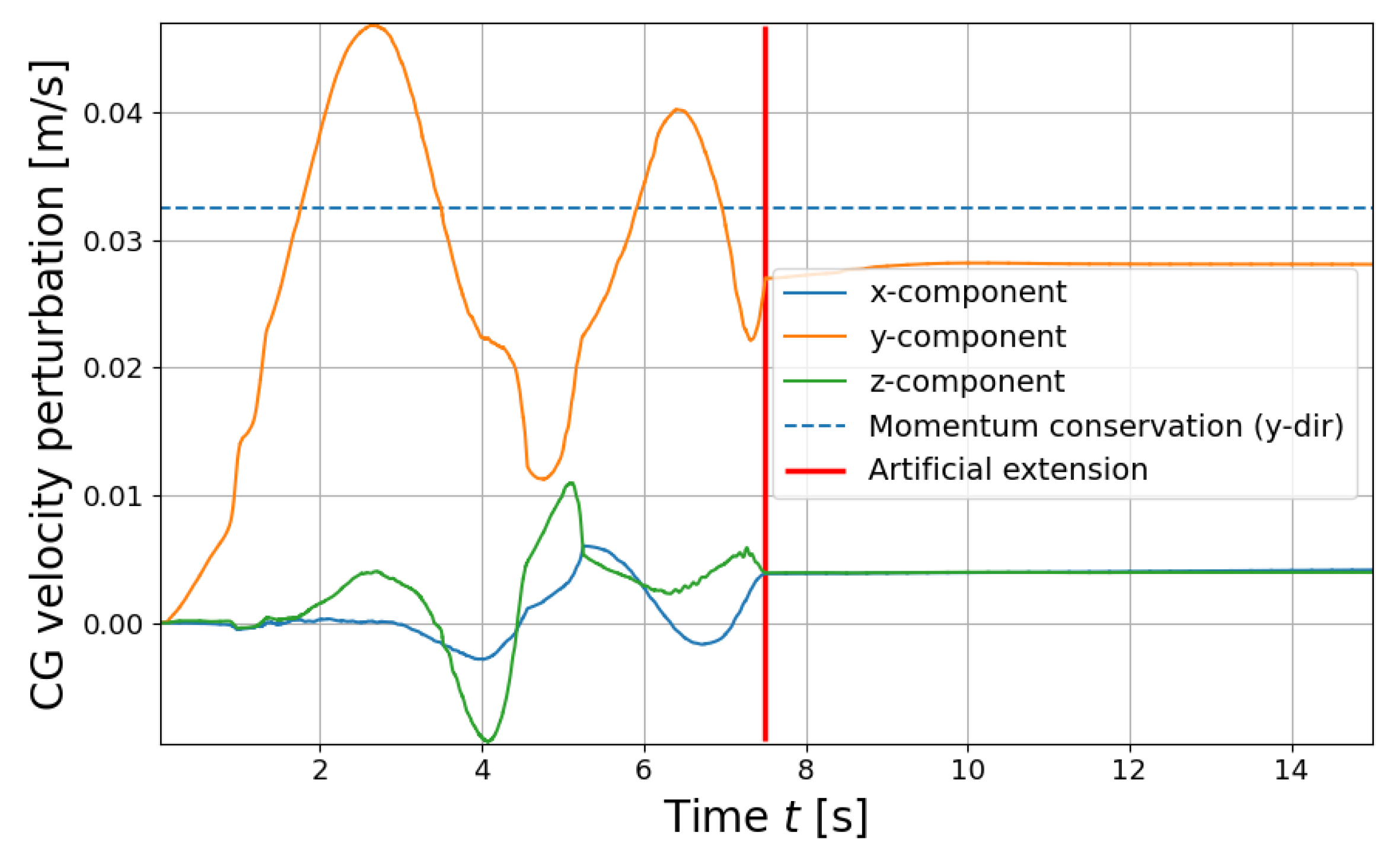
When the net impacts the space debris object, the contact forces (Figure 6) are fed into Equation (9) leading to the target’s translational dynamic reaction. For the purpose of this study, only the velocity is shown in Figure 8, with the addition of the analytical estimate of momentum conservation (for the y direction).

Figure 8. Space debris velocity CG reaction in the LVLH $\mathcal{L}$-frame due to the net contact dynamics.

As expected, the object’s velocity seems to oscillate around the analytical estimation of 32 mm/s of momentum exchange around the along-track direction. The artificial extension seems to result in a slightly underestimated final velocity of 28 mm/s, which would lead the Envisat to vary its y position by 0.40 m after 15 s. Although small, it is essential to limit the deviation in position with the use of a robust control system to avoid significant positional corrections. However, from this point of view, translational dynamics seem to result in limited risks.

3.3.2. Rotational Dynamics Risks

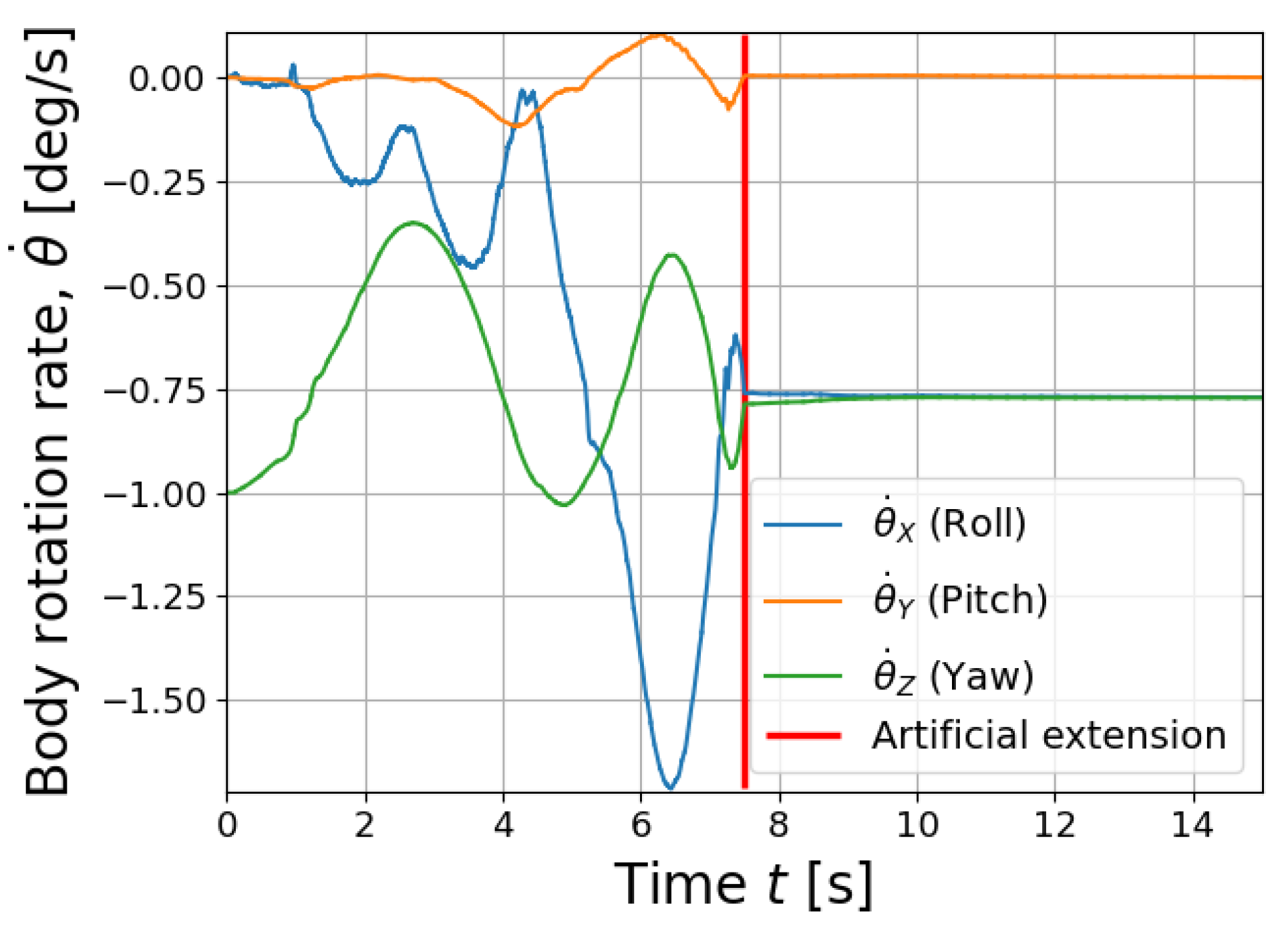
The second step is to analyse the effect of the contact moments (Figure 7) on the single- (Figure 9) and two-body (Figure 10) dynamics of the Envisat.

Figure 9. Debris body-frame self-rotation velocity ${\dot{\mathit{\theta }}}_{\mathrm{d}}$ due to the net contact dynamics.

Figure 10. Two-body debris body-frame self-rotation velocity ${\dot{\mathit{\theta }}}_{\mathrm{d}}$ due to the net contact dynamics.

When Envisat is simplified into a single rigid body, the net contact dynamics result in a slight damping of the object’s rotational rate (Z direction) by $0.25\mathrm{deg}/\mathrm{s}$, but it also leads to an increase of $1.75\mathrm{deg}/\mathrm{s}$ in the roll direction (where the inertia term is the lowest). The inclusion of solar array dynamics, and therefore a coupling term, worsens the situation in which not only the yaw dampening is non-existent but also the Envisat’s roll and pitch rotations are significantly increased. These may result in a pulley effect [27] between the chaser and target, in which the lower-mass chaser is propelled towards the target leading to a collision.

3.3.3. Solar Array Dynamics Risks

The solar array dynamics can be found in Figure 11. With a maximum solar array deviation of −8 deg, the lateral positional deviation of the array inside the net is $2.23\mathrm{m}$. With this type of significant deflection, the thin solar array could either break due to increased periodical stress or/and the net itself could tear resulting in a freely oscillating array. In the case of net tearing, the free solar array vibrations could result in breaking at the primary hinge location resulting in the creation of a large, significant piece of secondary space debris.

Figure 11. Solar array angular deflection and velocity.

The severity of the dynamic results is accentuated by the loads encountered by the primary solar array hinge, as depicted in Figure 12. Here, $M_{S_{h_i}}$ denotes the elements of ${\mathit{M}}_S$ in the local frame of the hinge.

Figure 12. Structural hinge moment loading, ${\mathit{M}}_{s_H}$, in hinge frame due to the frontal net impact of $V_{net}=20$ m/s.

By omitting the initial impact loads, which do not have sufficient time to propagate in the material, structural moments of $\pm 4$ kNm ($M_{S_{h_1}}$) and $\pm 5$ kNm ($M_{S_{h_3}}$) are consistently experienced from $t\approx 0.25$ s onwards. With an allowable limit, for the hinge–panel interface (location 1, see Figure 5), ranging from 200–1000 Nm [18], the results show a high likelihood of breaking and loss of structural integrity. Therefore, the frontal net impact results in the generation of a large secondary space debris object of $5\times 14.3\mathrm{m}$-size.

3.4. Structural Risks

Before presenting in depth the structural risks related to Envisat, the case of the ASAR antenna is briefly mentioned. In fact, structural failure of the ASAR is not expected. This is due to two main reasons. The first reason is that the ASAR is rigidly attached to the main Evisat body with a number of joints that distribute the experienced loading [28]. The second reason relates to the ASAR’s relatively large cross-sectional geometry, with a width and approximate thickness of $1.5\mathrm{m}$ and $0.156\mathrm{m}$ [28], respectively. Due to this, maximum compression and shear loads of $2000\mathrm{N}$ and $750\mathrm{N}$ resulted in only a maximum compression and shear stress of $8.55\mathrm{kPa}$ and $2.78\mathrm{kPa}$ [18]. Additionally, the maximum bending stress at the joints’ location has been found to be low (three orders of magnitude below the allowable stress).

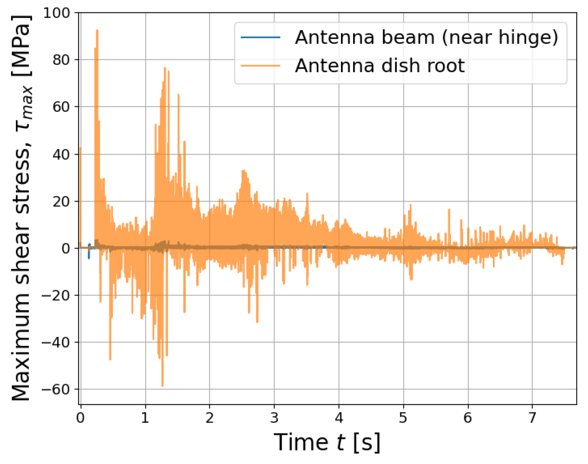
Lastly, in the case of structural risks, the identified weak locations (3 and 4, see Figure 5) of potential failure for the Ka-band antenna were checked for bending (Figure 13) and shear (Figure 14) failure from the aforementioned structural forces and moments.

Figure 13. Maximum normal stress (bending and axial combined) of the Ka-band antenna at two locations (hinge: 3, dish root: 4) as a function of time.

Figure 14. Maximum shear stress (torque and linear combined) of the Ka-band antenna at two locations (hinge: 3, dish root: 4) as a function of time.

The antenna or DRS structure of the Envisat can be assumed to be a combination of titanium alloy (TiGAI4V) [29] and CFRP (carbon fibre-reinforced polymer) [30], with associated ultimate limits for normal and shear stresses of ($950,3500$) MPa and ($50,100$) MPa [31,32], respectively. Whereas the normal stress limit is not attained, the range of shear stress values at the antenna–dish interface [33] is already reached within 1 s (Figure 14). Thus, secondary space debris is generated in the form of a $0.9\times 1$ m antenna dish [33].

3.5. Energy and Work Validation

With the decoupling of the implemented models within the aforementioned sequential modelling strategy, both the energy of the tethered net and the spacecraft must be checked individually.

Starting with the tether–net system, the net’s mechanical energy (here denoted as partial total energy) is plotted for this case study in Figure 15.

Figure 15. Total partial or mechanical energy of the net during the impact and capturing process as a function of time. Alongside the latter are the kinetic and elastic energies.

Initially, it can be observed that the energy of the net decreases due to the net deployment energy damping, similar to what was observed in [10,15]. Furthermore, the total partial energy is observed to strongly drop at $0.9\mathrm{s}$, $4.5\mathrm{s}$ and $5.25\mathrm{s}$. These are due to the energy loss caused by the damping process of contact and the decrease in the bullets’ velocity. After the last significant step decrease at $5.25\mathrm{s}$, the mechanical energy continues to decrease due to the net wrapping around Envisat being in continuous contact, and thus, contact and net damping.

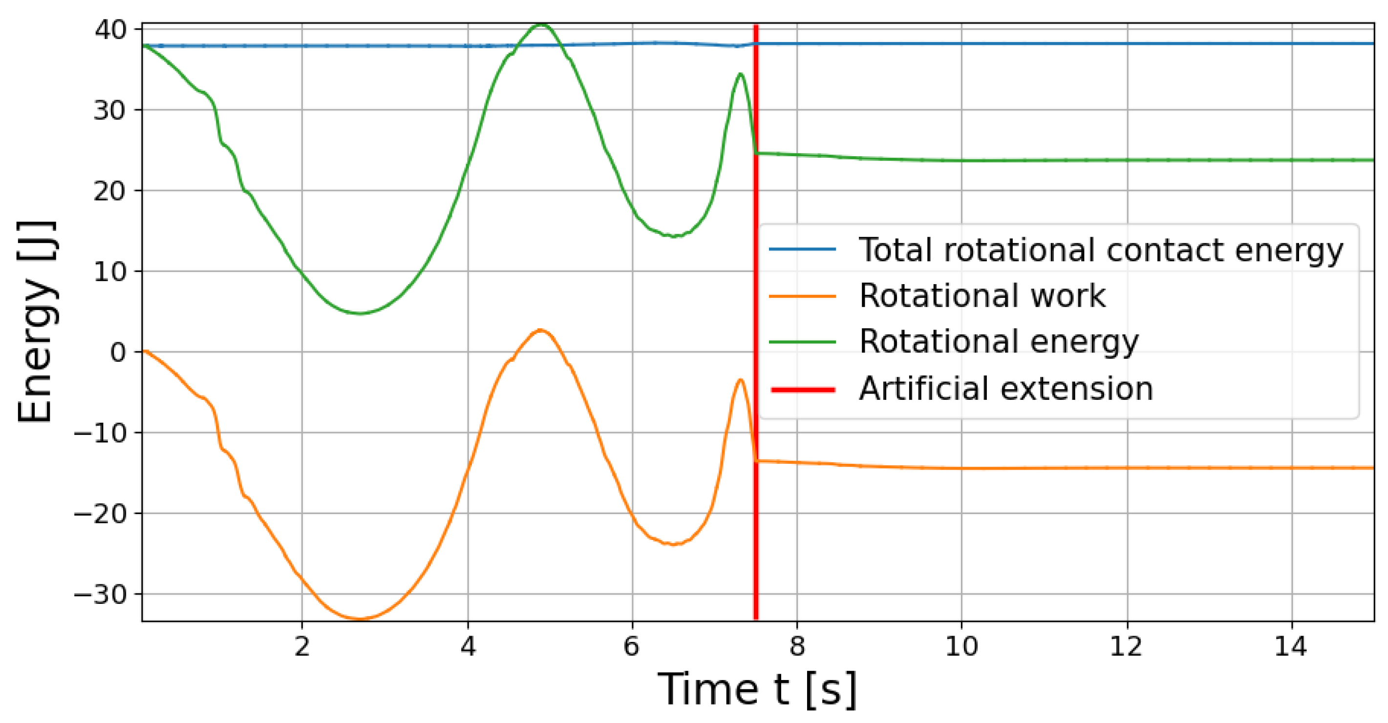
The last validation step is related to Envisat’s rotational energy as can be seen in Figure 16. The same has been performed for the translational kinetic energy, with the addition of model verification tests using a simplified constant force and moment case for verification. However, for the sake of brevity, only the rotational energy is presented in this paper.

Figure 16. Total rotational energy of Envisat during the impact and capturing process as a function of time. Alongside the latter is the rotational energy and contact moment dissipation work.

Three essential aspects can be observed in Figure 16:

• Total rotational energy is approximately constant with a maximum variation of 1 J at $t\approx 7.1\mathrm{s}$.
• Due to the rotational instability around the X-axis and the predicted effect of the modelling strategy itself, the rotational energy exceeds the total rotational energy from $4.5\mathrm{s}$ to $5.2\mathrm{s}$ by ∼$5\%$.
• The system’s energy is entirely conserved without variation during the artificial extension from $t=7.5\mathrm{s}$.

As was mentioned in Section 2.6, (1) and (2) were expected due to the fact that the modelling strategy assumptions resulted in a small violation of momentum and energy conservation. Additionally, this effect is related to the contact dynamics themselves, which have been found in the literature [15] to be unstable due to their high dependence on initial impact penetration $\delta$. However, due to the significant difference in mass between the net and the Envisat, this effect can be seen to be negligible. The correct implementation of the modelling strategy is confirmed by (3), as during this artificial extension, the net’s impact forces are exponentially decreased and Envisat’s dynamics are dominated by its initial conditions from $t=7.5\mathrm{s}$ onwards.

4. Conclusions and Perspectives

In this study, the effects of the contact dynamics of a capturing net on an Envisat mock-up have been analysed in terms of their potential for generating secondary space debris. To simulate such an event, a sequential modelling strategy is implemented which decouples the net dynamics model from the Envisat translational and rotational dynamics. Furthermore, the Envisat geometry is significantly simplified in order to simplify the modelling implementation and focus on its long flexible appendages.

To verify if structural failure occurs, a specific case study is chosen. This implies a frontal $30\times 30$ m net impact with a relative velocity of 20 m/s onto an Envisat mock-up. The net is discretised with point masses using the lumped mass or Multi-Spring-Damper model, in which the net threads were only allowed to experience tensile stresses. The simulation results implied that two of the three main long appendages of Envisat, namely the solar array and the Ka-band antenna, have a significant likelihood of breaking during the impact and wrapping process. Thus, a major conclusion from this study is that net capturing is riskier than originally expected.

Given the severity of these results, we highly recommend analysis of the effect of ejection parameters (i.e., impact velocity) and to improve the dynamic modelling by (1) removing the sequential nature of the modelling strategy, (2) improving the internal net dynamics to include bending stiffness, (3) providing an experimental approach to estimate the contact dynamics constant for net impacts and (4) validating the computed structural forces and stresses by applying more accurate Finite Elements Methods.

Appendix A.1. Modelling Strategy Graphical Representation

The graphical representation of the modelling strategy is represented in Figure A1.

Figure A1. Graphical representation of the sequential modelling strategy decoupling the three main models used.

Figure A1. Graphical representation of the sequential modelling strategy decoupling the three main models used.

Appendix A.2. Detection Strategy Graphical Representation

The graphical representation of the contact detection algorithm can be found in Figure A2.

Figure A2. Contact detection scheme diagram.

Figure A2. Contact detection scheme diagram.

References

- NASA. Orbital Debris Quarterly News, Volume 26—Issue 1. 2022. Available online: https://orbitaldebris.jsc.nasa.gov/quarterly-news/ (accessed on 25 December 2022).
- Shan, M.; Guo, J.; Gill, E. Review and comparison of active space debris capturing and removal methods. Prog. Aerosp. Sci. 2016, 80, 18–32. [Google Scholar] [CrossRef]
- Formiga, J.K.S.; dos Santos, D.P.S.; de Almeida Prado, A.F.B.; de Moraes, R.V.; Diaz, J.A.A. Ground-based laser effect on space debris maneuvering. Eur. Phys. J. Spec. Top. 2023, 232, 3059–3072. [Google Scholar] [CrossRef]
- Yang, L.; Zhang, Q.; Zhen, M.; Liu, H. “Dynamics and Design of Space Nets for Orbital Capture”; Springer-Verlag GmbH: Berlin/Heidelberg, Germany, 2017. [Google Scholar]
- Mankala, K.K.; Agrawal, S.K. Dynamic modeling and simulation of satellite tethered systems. J. Vib. Acoust. 2005, 127, 144–156. [Google Scholar] [CrossRef]
- Gao, S.; Yin, Y.; Sun, X.; Sun, Y. Dynamic simulation of fishing net based on cubic B-spline surface. Commun. Comput. Inf. Sci. 2012, 325, 141–148. [Google Scholar] [CrossRef]
- Benvenuto, R.; Lavagna, M.; Salvi, S. Multibody dynamics driving GNC and system design in tethered nets for active debris removal. Adv. Space Res. 2016, 58, 45–63. [Google Scholar] [CrossRef]
- Benvenuto, R.; Salvi, S.; Lavagna, M. Dynamics analysis and GNC design of flexible systems for space debris active removal. Acta Astronaut. 2015, 110, 247–265. [Google Scholar] [CrossRef]
- Botta, E.M.; Sharf, I.; Misra, A.K. Energy and momentum analysis of the deployment dynamics of nets in space. Acta Astronaut. 2017, 140, 554–564. [Google Scholar] [CrossRef]
- Botta, E.M. Deployment and Capture Dynamics of Tether-Nets for Active Space Debris Removal. Ph.D. Thesis, McGill University, Montreal, QC, Canada, 2018. [Google Scholar]
- Liu, L.; Shan, J.; Ren, Y.; Zhou, Z. Deployment dynamics of throw-net for active debris removal. In Proceedings of the 65th International Astronautical Congress, Toronto, ON, Canada, 29 September–3 October 2014. [Google Scholar]
- Shan, M.; Guo, J.; Gill, E. IAC-15-A6.5.7 An analysis of critical deployment parameters for tethered-net capturing for space debris removal. In Proceedings of the International Astronautical Congress, IAC, Jerusalem, Israel, 12–16 October 2015; Volume 3, pp. 2262–2267. [Google Scholar]
- Shan, M.; Guo, J.; Gill, E.; Gołȩbiowski, W. Validation of Space Net Deployment Modeling Methods Using Parabolic Flight Experiment. J. Guid. Control. Dyn. 2017, 40, 3319–3327. [Google Scholar] [CrossRef]
- Shan, M.; Guo, J.; Gill, E. Contact Dynamics on Net Capturing of Tumbling Space Debris. J. Guid. Control Dyn. 2018, 41, 2063–2072. [Google Scholar] [CrossRef]
- Shan, M. Net Deployment and Contact Dynamics of Capturing Space Debris Objects. Ph.D. Thesis, Delft University of Technology, Delft, The Netherlands, 2018. [Google Scholar] [CrossRef]
- Salvi, S. Flexible Devices for Active Space Debris Removal: The Net Simulation Tool. Master’s Thesis, Politecnico Di Milano, Milan, Italy, 2014. [Google Scholar]
- Shan, M.; Guo, J.; Gill, E. Deployment dynamics of tethered-net for space debris removal. Acta Astronaut. 2017, 132, 293–302. [Google Scholar] [CrossRef]
- Cuadrat-Grzybowski, M. Risks of Secondary Space Debris Generation from Net Capturing in Active Space Debris Removal Missions. Master’s Thesis, Delft University of Technology, Delft, The Netherlands, 2023. [Google Scholar]
- Gao, Q.; Zhang, Q.; Feng, Z.; Tang, Q. Study on launch scheme of space-net capturing system. PLoS ONE 2017, 12, e0183770. [Google Scholar] [CrossRef]
- Chen, Q.; Zhang, Q.; Gao, Q.; Feng, Z.; Tang, Q.; Zhang, G. Design and optimization of a space net capture system based on a multi-objective evolutionary algorithm. Acta Astronaut. 2020, 167, 286–295. [Google Scholar] [CrossRef]
- Gilardi, G.; Sharf, I. Literature survey of contact dynamics modelling. Mech. Mach. Theory 2002, 37, 1213–1239. [Google Scholar] [CrossRef]
- Shan, M.; Guo, J.; Gill, E. Contact Dynamic Models of Space Debris Capturing Using A Net. Acta Astronaut. 2017, 158, 198–205. [Google Scholar] [CrossRef]
- Si, J.; Pang, Z.; Du, Z.; Cheng, C. Dynamics modeling and simulation of self-collision of tether-net for space debris removal. Adv. Space Res. 2019, 64, 1675–1687. [Google Scholar] [CrossRef]
- Clohessy, W.H.; Wiltshire, R.S. Terminal Guidance System for Satellite Rendezvous. J. Aerosp. Sci. 1960, 27, 653–658. [Google Scholar] [CrossRef]
- Allard, C.; Schaub, H.; Piggott, S. General hinged rigid-body dynamics approximating first-order spacecraft solar panel flexing. J. Spacecr. Rocket. 2018, 55, 1290–1298. [Google Scholar] [CrossRef]
- Lacoursière, C. A Regularized Time Stepper for Multibody Systems; Department of Computing Science, Umeaa University: Umeå, Sweden, 2006. [Google Scholar]
- Shan, M.; Shi, L. Post-capture control of a tumbling space debris via tether tension. Acta Astronaut. 2021, 180, 317–327. [Google Scholar] [CrossRef]
- ASAR Overview—Envisat Instruments, ESA. Available online: https://earth.esa.int/eogateway/instruments/asar/description (accessed on 20 March 2023).
- Serrano, J.; SanMillan, J.; Santiago, R. Antenna pointing mechanism for ESA ENVISAT polar platform. In Proceedings of the 30th Aerospace Mechanisms Symposium, Hampton, VA, USA, 15–17 May 1996. [Google Scholar]
- Wuxi Huaxin Radar Engineering CO., Ltd. HUAXIN ANTENNA|Products|Vehicle-Mounted Antenna. Available online: https://www.hxantenna.com/Home.html (accessed on 15 April 2023).
- Titanium Ti-6Al-4V—ASM Material Data Sheet. Available online: https://asm.matweb.com/search/SpecificMaterial.asp?bassnum=mtp641 (accessed on 10 September 2023).
- Mirdehghan, S.A. Fibrous Polymeric Composites; Woodhead Publishing: Sawston, UK, 2021; pp. 1–58. [Google Scholar] [CrossRef]
- Mas-Albaiges, J.; Huertas, L. Communicating with the Polar Platform/Envisat—The DRS Terminal. ESA Bull. 1996, 88, 58–65. [Google Scholar]
Figure 1.
The Envisat mock-up model, presented in both orientations labelled as (A,B), is situated in the context of a net capturing scenario (red dots represent the bullets) with an origin at O (chaser). In green is the ASAR, blue is the solar array and in white is the Ka-band antenna. The y direction represents the flight direction, the radial coordinate corresponds to the x direction and the z direction completes the frame.
Figure 2.
Representation of the coordinate system with origin O, y direction representing the direction of flight, the radial coordinate as x direction and the z direction completes the frame.
Figure 3.
Level 1 to 2 contact bounding boxes of a generic simulation scenario for both net (red dots represent the bullets) and target systems.
Figure 4.
Representation of reference frames, incorporating the inertial frame , the body-fixed and hinge frames for the target ( and ), and the chaser-attached O- frame (). The respective centres of gravity for the main body, solar array and the entire spacecraft are labelled as , and in the visualisation. The solar array arm or yoke is omitted for simplicity.
Figure 5.
Visualisation for computing structural loads, featuring the solar array weak location as a main example.
Figure 6.
Contact force time series in the -frame.
Figure 7.
Contact moment time series in the -frame.
Figure 8.
Space debris velocity CG reaction in the LVLH -frame due to the net contact dynamics.
Figure 9.
Debris body-frame self-rotation velocity due to the net contact dynamics.
Figure 10.
Two-body debris body-frame self-rotation velocity due to the net contact dynamics.
Figure 11.
Solar array angular deflection and velocity.
Figure 12.
Structural hinge moment loading, , in hinge frame due to the frontal net impact of m/s.
Figure 13.
Maximum normal stress (bending and axial combined) of the Ka-band antenna at two locations (hinge: 3, dish root: 4) as a function of time.
Figure 14.
Maximum shear stress (torque and linear combined) of the Ka-band antenna at two locations (hinge: 3, dish root: 4) as a function of time.
Figure 15.
Total partial or mechanical energy of the net during the impact and capturing process as a function of time. Alongside the latter are the kinetic and elastic energies.
Figure 16.
Total rotational energy of Envisat during the impact and capturing process as a function of time. Alongside the latter is the rotational energy and contact moment dissipation work.