An Integrated Monitoring, Diagnostics, and Prognostics System for Aero-Engines under Long-Term Performance Deterioration

Abstract

In the field of aircraft engine diagnostics, many advanced algorithms have been proposed over the last few years. However, there is still wide room for improvement, especially in the development of more integrated and complete engine health management systems to detect, identify, and forecast complex faults in a short time. Furthermore, it is necessary to ensure that these systems preserve their capabilities over time despite engine deterioration. This paper addresses these necessities by proposing an integrated system that considers the joint operation of feature extraction, anomaly detection, fault identification, and prognostic algorithms for engines with long operation times. To effectively reveal the actual engine condition, light adaptive degraded engine models are computed along with different health indicators that are used as inputs to train and test recognition and prediction models. The system is developed and evaluated using a specialized NASA platform which provides data from a turbofan engine fleet simultaneously experiencing long-term performance deterioration and faults. Contrary to other compared solutions, our results show that the proposed system is robust against the effects of engine deterioration, maintaining its level of detection, recognition, and prediction accuracy over a total engine service life. The low computational cost algorithms has generally fast performance in all stages, making the system suitable for online applications.

1. Introduction

All aero-engines experience gradual or sudden mechanical and performance degradation as a natural part of their useful life. Performance degradation can be classified as either short-term and long-term deterioration. The former is associated with recoverable deterioration such as compressor fouling, and performance can be retrieved through maintenance actions such as online and offline washings. The latter is related to irrecoverable structural degradation, for example, tip clearance increase in the turbine blades, and the performance can only be retrieved by repair or replacement of the damaged parts. For engines with long operation times, deterioration can remain present despite major overhauls. In any case, performance degradation will lead to an increase in the specific fuel consumption, exhaust gas temperature, and heat rate and a decrease in power, thermal efficiency, and thrust [1].

To address problems in gas turbines, the Condition-Based Maintenance (CBM) strategy has been adopted in the past with effective results. With the continuous evolution of technology in diverse areas, CBM has evolved into the Prognostics and Health Management (PHM) strategy. PHM describes engine health in a more integrated form than CBM, with an emphasis on early detection, improved current condition assessment, and prediction of faults. In this way, the PHM approach works jointly with the stages of data collection and preprocessing, feature extraction, monitoring (anomaly detection), diagnostics (fault identification), prognostics, and maintenance decision management.

The implementation of PHM in aviation can lower the incidence of faults in principal engine components and subsystems, thereby increasing aircraft safety and reducing operation and maintenance costs [2]. According to [3], engine failures were the second most causes of aircraft accidents from 2008 to 2017. For this reason, the continuous verification of aeronautical regulations and standards to improve safety in aero-engines makes evident the necessity to implement more efficient PHM systems.

A great variety of algorithms for each PHM stage have been separately developed in recent years, taking advantage of the progress in machine learning and deep learning research. Comprehensive reviews about this progress, such as [4,5,6,7], can be found in the literature. Recently, researchers have focused on deep learning methods such as recurrent neural networks (RNNs) and convolutional neural networks (CNNs) in order to exploit their powerful feature learning and classification/prediction capabilities for use within PHM strategies in rotating machinery [8], in particular for aircraft engines. For example, Fentaye et al. [9] presented a CNN-based fault detection and isolation method for a three-shaft turbofan engine in which a physics-driven performance trend monitoring system produced gas path fault signatures to train the network. In [10], the authors developed a hybrid framework by combining a physics-based model and data-driven algorithms based on deep learning architectures to overcome the limitations of both approaches. The method was applied to predict run-to-failure deterioration trajectories from a fleet of turbofan engines under varying operating conditions. Dong et al. [11] and Zhang et al. [12] worked with long short-term memory (LSTM) networks to forecast the remaining useful life of engines from a commercial turbofan model. Using state-of-the-art machine learning and deep learning techniques such as LSTM, Baptista et al. [13] proposed a data-driven classification approach to address the problem of prognostics applied to two real-world aviation case studies, one for describing the fault progression of a critical component in a gas turbine and the other one for describing engine reliability.

Despite the advances in this area, the full deployment of PHM faces challenges in practice [14]. For aircraft engines more specifically, we highlight the following two needs:

• The integration of new artificial intelligence methodologies and PHM frameworks has been one of the main goals in aircraft engine health management, as it can help to better describe and predict the complex nature of aero-engine faults and deterioration. Several recent works have proposed the joint operation of typical PHM methodologies with other stages, such as fault severity estimation, deterioration prognostics, and innovative remaining useful life estimation approaches [15,16,17,18]. However, due to the complexity of combining different algorithms to efficiently interact with each other and the creation of multiple system configurations, it is necessary to continue to develop and improve such unified solutions by taking advantage of progress in machine learning and deep learning.
• PHM systems have to deal with a number of issues, for example, measurement uncertainties, nonlinearity of the diagnostic problem, limited availability of sensors, occurrence of multiple faults, varying operating conditions, unavailability of data, etc. Among these elements, measurement uncertainties have a great impact on diagnostic accuracy, as they result in incorrect information about the presence and magnitude of deterioration and faults, causing misinterpretation of the engine health assessment. Measurement uncertainties are present in the form of random noise (related to the operating environment) and sensor bias (due to instrumentation faults). A robust PHM system should not lose its ability to track and reveal faults due to background uncertainties.
  Because of the limited availability of fault data, many algorithms are tested and validated using short periods of engine operation during which the deterioration level does not significantly change. Therefore, the diagnostic accuracy of the algorithms is not affected by the noise associated with deterioration. However, as uncertainties increase with engine aging, algorithms can lose their ability to discriminate among faults, deterioration, and noise signals if health indicators fail to reveal the engine condition. Thus, the continuous verification of such indicators to preserve their quality during long operation times is of great importance.

As a contribution to solving the above aspects, this work proposes an integrated PHM architecture for aero-engines that preserves its recognition and prediction capabilities despite long-term deterioration effects. The system is based on three principal algorithms: (1) feature extraction, (2) anomaly detection and fault identification, and (3) deterioration and fault prognostics. To reveal trends and the current engine condition, different health indicators (residuals) are computed. The main indicator is based on computationally light adaptive degraded engine models (ADEM) that capture the current level of deterioration to reduce the baseline model inadequacy with progressive engine degradation while maintaining the level of diagnostic and prognostic accuracy over time.

The proposed PHM system was developed and tested using the NASA platform called ProDiMES (Propulsion Diagnostic Method Evaluation Strategy) [19], which promotes fair competition among diagnostic methodologies and further development of PHM systems for aero-engines [20,21,22,23,24]. This software contains a realistic simulation of a fleet of commercial two-spool turbofan engines which experience different levels of performance deterioration and faults. The software outputs are measured parameter histories at cruise and take-off regimes registered for each engine and flight cycle in the fleet. The presence of both short-term and long-term deterioration is considered as a natural part of engine operation due to fouling and erosion in major components. Faults are non-expected scenarios in a rapid or abrupt form, and are present in components, sensors, and actuators. ProDiMES assists in the computation of performance metrics to evaluate the detection and classification capabilities of the algorithms. In this paper, the internal algorithms of the system are compared with the performance results of other published approaches using ProDiMES, allowing for validation of the correct functionality and effectiveness of the complete system during a total engine service life.

2. Baseline Model Inadequacy for Long-Term Diagnostics

ProDiMES produces engine flight time series snapshots, each representing the averaged values of sensed variables recorded periodically by a measurement system during an entire flight cycle. For one snapshot, seven measured variables and four operating conditions are registered with their respective noise level. These measurements are separately collected at takeoff and cruise regimes during a flight cycle. ProDiMES provides a wide variety of realistic and unique operating histories through the variation of deterioration profiles, flight conditions (Mach number, pressure altitude, ambient temperature, power setting), and fault scenarios. When the data have been generated, users are able to develop and evaluate different gas path diagnostic approaches.

Typically, a gas turbine diagnostic procedure employs health indicators in the form of residuals or deviations. The quality of residuals with regard to revealing faults depends on the reference sample and the correct implementation of baseline models of healthy engine performance. For example, a representative engine fleet dataset from ProDiMES with 100 healthy engines and 90 initial flights per engine is sufficient to create a typical fleet-average baseline model (FAM) [21]. Such an FAM can be created using a second-order polynomial function for which the matrix of unknown coefficients $\widehat{\mathbf{X}}$ of size $(t\times m)$ is computed using the least squares method:

$$\widehat{\mathbf{X}}={\left({\mathbf{C}}_u^T{\mathbf{C}}_u\right)}^{-1}{\mathbf{C}}_u^T{\mathbf{Y}}_0$$

(1)

where ${\mathbf{C}}_u$ is a matrix of size $(f\times t)$ for f total consecutive flight cycles and t terms $(1,u_1,u_2,\dots ,u_1{u}_2,\dots ,u_3^2,u_4^2)$ that combine elements from a vector $\mathbf{U}$ of four operating conditions set by ambient and control variables (see

Table A1. Operating conditions u [19].

ID	Symbol	Description	Units
1	Nf	Physical fan speed	rpm
2	P2	Total pressure at fan inlet	psia
3	T2	Total temperature at fan inlet	°R
4	Pamb	Ambient pressure	psia

), while ${\mathbf{Y}}_0$ is a matrix of size $(f\times m)$ of m measured variables corresponding to a standard measurement system (see

Table A2. Measured variables Y [19].

ID	Symbol	Description	Units
1	Nc	Physical core speed	rpm
2	P24	Total pressure at LPC outlet	psia
3	Ps30	Static pressure at HPC outlet	psia
4	T24	Total temperature at LPC outlet	°R
5	T30	Total temperature at HPC outlet	°R
6	T48	Total temperature at HPT outlet	°R
7	Wf	Fuel flow	pps

). After obtaining the coefficients x, a baseline function for all measured variables is determined as ${\mathbf{Y}}_{0FAM}={\mathbf{C}}_u·\widehat{\mathbf{X}}$. The residuals $R_{FAM}$ are then computed as relative differences between the actual measured values $Y^{*}$ and the baseline values $Y_{0FAM}\left(\mathbf{U}\right)$.

Because applying FAM to engines with different operating conditions does not correctly reflect the individual performance and level of deterioration of each engine, a corrected fleet-average baseline model (CFAM) is employed [21]. The new scheme considers $Y_0$ from FAM and an average correction coefficient formed of residuals from the first n flights without faults in each engine. Considering one measured variable, CFAM is expressed as follows:

$$Y_{0CFAM}=Y_{0FAM}(1+\frac{1}{n}\sum _{j=1}^n{R}_{FA{M}_j})$$

(2)

In this way, the corrected residuals $R_{CFAM}$ are computed in the same manner as $R_{FAM}$. For fault recognition, residuals are called patterns and are normalized by dividing them by a coefficient based on the standard deviation of random errors $\sigma$.

In other studies using ProDiMES [21,23,25], CFAM was employed to diagnose faulty engines during a short time (approximately 50 flights). The model conserved its accuracy, as the deterioration level was constant within this interval. However, this approach is not suitable when applied to long operation times, as engine deterioration changes considerably over time. This affects the accuracy of CFAM and quality of the residuals, resulting in incorrect fault diagnostics. Figure 1 depicts the baseline model’s inadequacy with progressive deterioration. Figure 1a shows the residuals R for a temperature variable Y (T24—low-pressure compressor outlet, Table A2) and 5000 flight cycles of an engine, while Figure 1b displays the corresponding random errors or uncertainties $ϵ$. Although a performance degradation trend (an increase in the temperature) is correctly captured by the residuals, the errors grow as time passes and are more evident at the final stage of the engine’s life. This problem arises because the influence of the operating conditions on the measured variables of the degraded engine is increasingly different from the influence of the baseline model, with constant coefficients producing a less accurate model for computing residuals. This is important because the signals produced by an unavoidable and progressive deterioration in the machinery can be confused as fault signals, and vice versa, especially in aged engines.

It is clear that the CFAM approach is not suitable for long-term diagnosis and that a new one is required to ensure that diagnostic and prognostic decisions are not affected when faults appear in deteriorated engines. In the following sections, we attempt to overcome this problem by implementing adaptive degraded engine models into the feature extraction stage.

3. Proposed PHM System

This section presents the structure of the proposed system and describes how the algorithms interact with each other. The system is intended to produce flight-by-flight engine performance analysis during a full service life. It is composed of three main algorithms:

• Feature extraction
• Anomaly detection and fault identification
• Deterioration and fault prognostics

3.1. Feature Extraction Algorithm

Considering the structure of Equation (1), a baseline function with one measured variable and four operating conditions [23] has the following form:

$$Y_0\left(\mathbf{U}\right)=x_1+x_2{u}_1+x_3{u}_2+\dots +x_6{u}_1{u}_2+\dots +x_{15}{u}_4^2$$

(3)

As performance degradation is dependent on the engine’s operation time, a variable of the relative flight number $\overline{t}$, which is a measure of deterioration severity, is added to the arguments of the baseline function to produce a Degraded Engine Model (DEM) [17]:

$$Y_{DEM}(\mathbf{U},\overline{t})=Y_0\left(\mathbf{U}\right)+x_{16}\overline{t}$$

(4)

When the DEM is constant in the interval of analysis, it is called a Fixed Degraded Engine Model (FDEM); there are two of these, FDEM1 and FDEM2. If the coefficients of the DEM are updated with time, it is called an Adaptive Degraded Engine Model (ADEM). Residuals employing FDEM1 can reveal deterioration trends, and are employed by the deterioration prognostics algorithm. After the unknown model coefficients x have been determined using Equation (1), FDEM1 can be converted into a baseline function by setting $\overline{t}=0$ and obtaining residuals $R1$:

$$R1=\frac{Y-Y_{FDEM1}(\mathbf{U},\overline{t}=0)}{Y_{FDEM1}(\mathbf{U},\overline{t}=0)}.$$

(5)

In the same way, residuals $R2$ are computed as follows:

$$R2=\frac{Y-Y_{ADEM}(\mathbf{U},\overline{t})}{Y_{ADEM}(\mathbf{U},\overline{t})}.$$

(6)

The ADEM is computationally light and easily adapts to capture the current level of deterioration that grows with engine operation. Without the presence of faults, the signals from Equation (6) behave as random errors without any trend, as they are just differences between deterioration values. When a fault appears, the anomaly detection and fault identification algorithm verifies significant changes in $R2$ values to make a diagnostic decision. When the fault has been detected and identified, ADEM stops updating to become FDEM2 with the last adapted model coefficients (i.e., $ADE{M}_{last}=FDEM2$). From this moment on, the residuals are computed as follows:

$$R3=\frac{Y-Y_{FDEM2}(\mathbf{U},\overline{t})}{Y_{FDEM2}(\mathbf{U},\overline{t})}.$$

(7)

These last residuals are utilized in the fault diagnostics and prognostics algorithm. Residuals $R3$ contain both the influence of the long-term degradation accumulated over time and the influence of the fault, which is evolving at a certain rate.

For better diagnostic performance, all types of residuals are smoothed using an exponential moving average [25]:

$$R_{smoot{h}_{i,j}}=\alpha R_{i,j}+(1-\alpha )R_{smoot{h}_{i,j-1}}$$

(8)

where i is the measured variable, j is the current flight, and $\alpha$ is a factor with values 0 to 1 that controls the smoothing level.

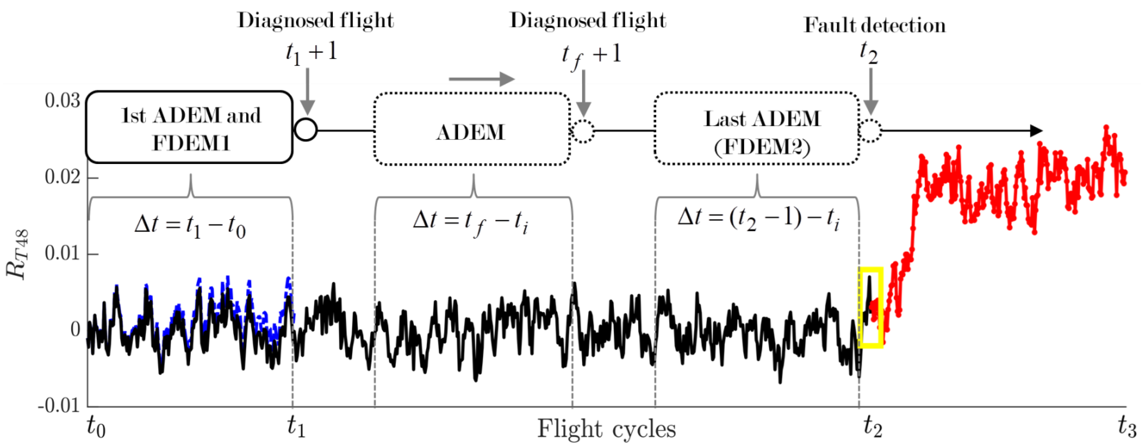
Figure 2 displays an example of the system as a function of flight cycles t, showing the behavior of the residuals for a temperature variable ($T48$—temperature at high-pressure compressor outlet, Table A2). The total interval of the engine performance analysis ($t_0,t_3$) is partitioned into three intervals:

• Interval 1 ($t_0,t_1$). The feature extraction algorithm is active from the beginning of the monitoring analysis and lasts until it ends. Because at initial engine operation there are insufficient data to create an adequate degradation model, a pre-built CFAM with different healthy engines is implemented to obtain the required residuals for monitoring and diagnostics. As mentioned before, CFAM can be effectively applied for a short time in low-degradation cases. FDEM1, the first ADEM, and the corresponding residuals are only available when flight $t_1$ is reached, and use the data that have been accumulated in the interval $\Delta t=t_f-t_i$, where $t_i$ and $t_f$ are the initial and final flights coinciding with $t_0$ and $t_1$, respectively. Figure 3 is a close-up of Interval 1; the similar behavior of the three types of residuals can be observed, confirming that CFAM can temporarily replace FDEM and ADEM.
• Interval 2 ($t_1+1,t_2$). FDEM1 is computed at $t_1$, and does not change throughout the entire second interval. Residuals $R1$ and $R2$ begin to separate from each other after $t_1$ due to the deterioration growth captured by residuals $R1$ (manifested, for example, by the increase of temperature). The deterioration prognostics algorithm receives these last residuals to train a deep neural network and forecast the deterioration behavior.
  As for residuals $R2$, the first ADEM is also obtained at $t_1$, then the model coefficients are constantly renewed by shifting the measured variables and operating conditions according to the currently diagnosed flight using the interval $\Delta t=t_f-t_i$ that precedes it. The optimal number of required flights $\Delta t$ is selected based on the model’s accuracy after testing different values (in this paper, $\Delta t=200$). Because each update involves the last flights, ADEM is always adapted to the current level of engine deterioration, producing an adequate reference function in the computation of residuals $R2$. The model stops updating at $t_2$ after a fault is detected by the anomaly detection and fault identification algorithm. From the start of engine monitoring, this algorithm needs a pretrained neural network with CFAM-based residuals in order to recognize a variety of fault classes, including healthy cases. Figure 4 schematizes how the FDEM and ADEM are created over time from $t_0$ to $t_2$.
• Interval 3 ($t_2+1,t_3$). When a fault is detected, FDEM2 (the last ADEM) remains the same throughout Interval 3 to compute residuals $R3$. As before, the same type of deep neural network is employed to predict the behavior of the fault, which evolves along with the deterioration. In practice, the fault prognosis analysis should be performed within a short period in order to take rapid maintenance actions. When an engine presents no faults or only small faults that are impossible to detect and identify, the monitoring system remains in active operation to the end of the engine’s service life.

3.2. Anomaly Detection and Fault Identification Algorithm

3.2.1. Fault Recognition Technique

In the proposed system, the anomaly detection and fault identification stages are viewed as a single recognition problem. This means that only one classifier is trained to recognize the current state among 19 different classes (the no-fault case and 18 fault scenarios). If a pattern has similarities to the trained signals from engines without faults, then the pattern is classified as a healthy class; otherwise, it belongs to one of the fault scenarios, confirming the detection of a problem and identifying the type of fault at the same time. In any case, the current condition can only be associated with one class. This is performed by the selected pattern recognition technique, which determines internal frontiers between each class, including a healthy engine class. Thus, no direct threshold is assigned and applied to the residuals. To control the balance between the True Negative Rate (TNR) and the True Positive Rate (and the true classification probabilities), the number of patterns in each class is changed. For example, to raise TNR, the number of patterns in a healthy engine class should be increased.

Metrics for detection, classification, and detection latency are computed to evaluate the performance of the classifier (see Appendix B) [19]. A regularized extreme learning machine (RELM) is selected for this joint task. RELM has proven to be superior in the three mentioned metrics compared to other tested recognition methods employed for aircraft engine gas path diagnostics [23]. In comparison with other typical neural networks, such as multi-layer perceptron and radial basis networks, the main characteristics of RELM are: (1) only the output layer parameters are computed, while the hidden layer parameters are randomly selected; and (2) only the computation of a matrix inverse is required, meaning that there is no need for a back-propagation algorithm with learning iterations for error minimization. For this reason, the technique is simple to construct and fast to train.

Consider the training dataset ${({\mathbf{R}}_j,{\mathbf{o}}_j)}_{j=1}^N$ with N samples, where ${\mathbf{R}}_j={[R_{j1},R_{j2},\dots ,R_{jm}]}^T$ is a vector of residuals with m measured variables and ${\mathbf{o}}_j={[o_{j1},o_{j2},\dots ,o_{jq}]}^T$ is the corresponding desired output vector, which is associated with labels 1 and −1 to indicate which of the q classes the residual vector belongs to. The estimated network output $\widehat{\mathbf{o}}$, with L hidden layer neurons and an activation function $g\left({\mathbf{R}}_j\right)$, is provided by:

$${\widehat{\mathbf{o}}}_j=\sum _{i=1}^{L}g({\mathbf{w}}_i^T{\mathbf{R}}_j+b_i){\beta }_i$$

(9)

where $b_i$ is the bias value and ${\mathbf{w}}_i={[w_{i1},w_{i2},\dots ,w_{im}]}^T$ and ${\beta }_i={[{\beta }_{i1},{\beta }_{i2},\dots ,{\beta }_{iq}]}^T$ are the hidden and output layer weights, respectively. Equation (9) can be expressed as $\widehat{\mathbf{o}}=\mathbf{H}\widehat{\beta }$ with matrices $\mathbf{H}=[g({\mathbf{w}}_1^T{\mathbf{R}}_1+b_1),\dots ,g({\mathbf{w}}_L^T{\mathbf{R}}_N+b_L)]$ and $\beta ={[{\beta }_1,\dots ,{\beta }_L]}^T$. For the target matrix $\mathbf{O}={[{\mathbf{o}}_1^T,\dots ,{\mathbf{o}}_N^T]}^T$, the problem to solve is defined as $\arg {min}_{\beta }{\parallel \mathbf{H}\beta -\mathbf{O}\parallel }_F$, which means finding output layer weights that minimize the difference between outputs and targets. This last expression is a least squares method problem; the solution is provided by $\widehat{\beta }={\mathbf{H}}^{†}\mathbf{O}$, where ${\mathbf{H}}^{†}$ is the pseudo-inverse of $\mathbf{H}$. However, due to the numerical instability of ${\mathbf{H}}^{†}$, a regularized version can be employed instead to optimize the solution [26]:

$$\arg \underset{\beta }{min}{\parallel \mathbf{H}\beta -\mathbf{O}\parallel }_F+\frac{1}{\lambda }{\parallel \beta \parallel }_F.$$

(10)

Here, the parameter $\lambda$ maintains a balance between the training error and the regularization term. Because different values of $\lambda$ produce different hyperplanes of separation, the leave-one-out cross-validation approach is utilized to find the optimal value. Depending on L and N, the output weights are obtained with:

$$\begin{array}{c}\hfill \widehat{\beta }={({\mathbf{H}}^T\mathbf{H}+{\lambda }_{opt}\mathbf{I})}^{-1}{\mathbf{H}}^T\mathbf{O}\mathrm{if}L<N\mathrm{or}\\ \hfill \widehat{\beta }={\mathbf{H}}^T{(\mathbf{H}{\mathbf{H}}^T+{\lambda }_{opt}\mathbf{I})}^{-1}\mathbf{O}\mathrm{if}L\ge N,\end{array}$$

(11)

where $\mathbf{I}$ is the identity matrix. Finally, after using the expression $\widehat{\mathbf{o}}=\mathbf{H}\widehat{\beta }$, the classification of an input vector is obtained with $\mathrm{Label}\left(\mathbf{R}\right)=\arg {max}_{d=1\dots q}\left(\widehat{\mathbf{o}}\right)$.

3.2.2. Anomaly Detection Rule

When a fault appears in a certain flight, RELM should detect it and identify it as soon as possible; however, due to network misclassifications, a single diagnosis is not sufficient for a final decision. ADEM continues to adapt if a fault is not detected and stops when the opposite happens, ensuring that the model does not absorb the fault influence, as this would produce a decrease in residuals $R2$ and an inability to identify current and future faults. If the model is stopped too soon or too late, the low quality of ADEM causes elevated rates of missed detections or false alarms, as well as negatively impacting the fault identification and prognosis stages. For this reason, adequate determination of the anomaly detection rule is critical for the system. Three different rules are proposed and evaluated. The first analyzes whether n consecutive fault occurrences of the same class type have occurred. Those flights presenting fault cases are included in the construction of the ADEM. The second rule works in the same manner, except that it excludes the fault scenarios from the model. The third excludes the fault cases from ADEM, then analyzes whether n occurrences (not necessarily consecutive ones) have occurred within a window of past flights, including the current analyzed flight.

Figure 5 better explains the third detection rule for an interval of 50 flights, analyzing three occurrences within a ten-flight window. The engine is under fault-free operation in the first 35 flights, with a fault occurrence at flight 36 which remains up to flight 50. The two subplots in the figure are interconnected, as for each flight there is a residual value (Figure 5a) that serves as input to a pretrained RELM that produces the corresponding classification of the pattern (Figure 5b). For simplicity, only the diagnoses of seven classes are displayed. Let us suppose that the current diagnosis is on flight 14 accompanied by a first window (Win 1). Because no problem has appeared in this interval, the no-fault scenario is correctly reflected by the residuals and classified by the network in most cases, with two false alarms associated with the Fan and LPC fault classes (triangles), which are excluded from the ADEM. Now, let us consider the current diagnosis at flight 40 with its corresponding window (Win 2). At this point, three nonconsecutive occurrences (circles) of the same class type have appeared, meaning that the detection is confirmed in the third event and identified as an HPC fault. ADEM is stopped from being renewed at flight 40, and the misdiagnoses found in the window are not considered in the model. From flights 41 to 50, it can be seen that the HPC fault continues to be correctly diagnosed by the network with only minor classification errors.

3.3. Prognostic Algorithm

The proposed system employs the LSTM architecture to forecast the behavior of both engine deterioration and faults. LSTM was selected for this task due to its proven effectiveness in learning long-term dependencies between time steps of sequence data. When used in prognostics problems, the general architecture of the network includes a sequence input layer (inputs as sequences or time series), an LSTM layer, a fully connected layer, and a regression output layer. More information about LSTM can be found, for example, in [27].

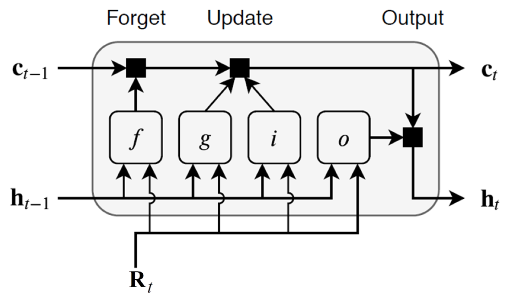
An LSTM layer works with a time series (in this case, either residuals $R1$ or $R3$) with m features and S time steps as input to the layer. Here, ${\mathbf{c}}_t$ and ${\mathbf{h}}_t$ correspond to the cell state and the hidden state with D units at time step t (flight), respectively. The cell state retains learned information from previous steps, while the hidden state is the output of the LSTM layer at a given time step. The first LSTM block receives the initial state and the first time step (vector of residuals) to produce the first output and the corresponding updated cell state. At step t, the output and the cell state are computed using the previous network state (${\mathbf{c}}_{t-1}$ and ${\mathbf{h}}_{t-1}$) and the next sequence step. At each time step, the LSTM layer adds or deletes information from the cell state through internal elements called gates, as shown in Figure 6. The forget gate f controls which information should be retained or discarded. The input gate i controls the level of cell state update. The cell state can be updated with the generated gate outputs. The output gate o decides what the next hidden state will be. After being computed, both the new ${\mathbf{c}}_t$ and the new ${\mathbf{h}}_t$ are carried over to the next time step. The gates ensure that only relevant information is transmitted through the sequence chain, resulting in improved predictions.

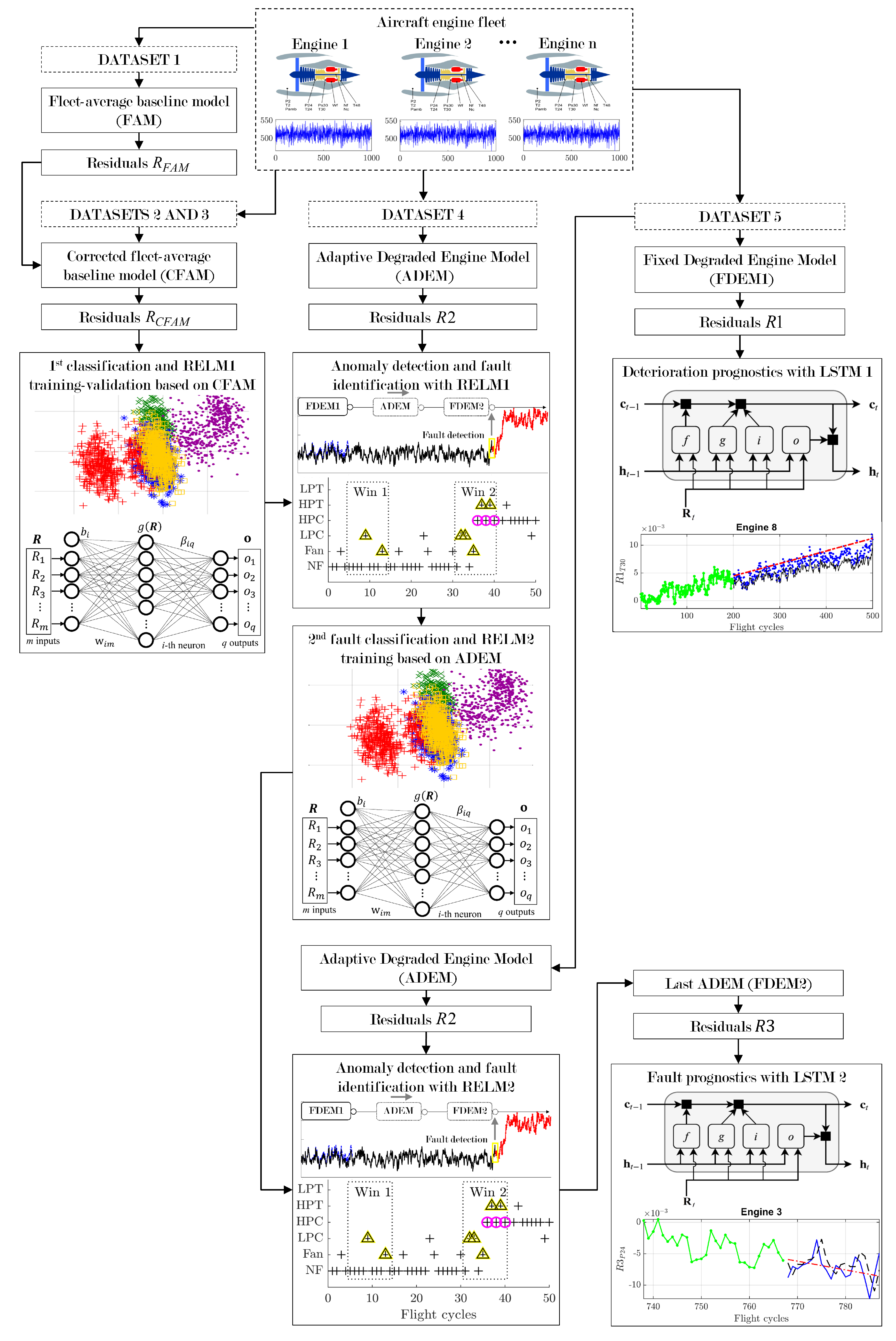
3.4. Datasets and Flowchart of the PHM System

Five datasets were generated through ProDiMES to develop and internally evaluate the system (

Table 1. Datasets for FAM creation and RELM training/validation.

Description	Set 1: FAM Creation	Sets 2–3: RELM1 Train-Val	Sets 4–5: RELM2 Train-Val
Number of health conditions	1	19	19
Engines per health condition	100	100	20
Flights per engine	5000	50	5000
Total number of engines	100	1900	380
Minimum initiation flight of fault initiation	None	11	250
Fault and evolution rate	None	Random	Random
Minimum Rapid fault evolution rate	None	9	9
Maximum fault evolution rate	None	9	100
Sensor noise	On	On	On

). The datasets contained flight cycles (with registered measured parameters and operating conditions) from different fleets with engines experiencing fault and no-fault conditions under cruise regimes as well as progressive deterioration. Based on the previous descriptions of the individual algorithms and techniques employed, Figure 7 displays the flowchart of the proposed system working with the generated datasets.

Dataset 1 was used for FAM creation with 100 healthy engines. Only the first 90 flights out of 5000 were used for the model, ensuring low degradation in the engines.

Datasets 2 and 3 were generated with the same characteristics, and were intended for constructing a training set and a validation set, respectively. Together, they constituted the first fault classification used for training and validating a preliminary classification network (RELM1) with corrected residuals using CFAM. The datasets had the same size. and each of them contained 95,000 flights (19 fault conditions × 100 engines per condition × 50 flights per engine), from which 19,000 were used for residual correction with the first ten flights in each engine and 76,000 were used for diagnostics. Because the number of flights for each engine was only 50, the level of deterioration was randomly selected through ProDiMES. In this way, RELM1 was trained with a representative classification containing all 19 health conditions and with different levels of deterioration that are possible in the fleet. As an important remark, RELM1 does not solve the problem of reduced recognition accuracy due to the baseline model’s inadequacy in long-term diagnostics; however, it can assist in recognizing fault conditions from the beginning of monitoring analysis and during the first implementation of the ADEM-based procedure. The optimal network training configurations were found by the trial-and-error method, with different architectures tested to obtain the one with the highest classification accuracy value. For RELM1, the network size was 7 (measured variables as inputs) × 6000 (hidden neurons) × 19 (fault scenarios as output neurons), ${\lambda }_{opt}$ = 0.4493, the size of output layer weight matrix $\beta$ was 19 classes × 6000 hidden neurons, and the size of target matrix $\mathbf{O}$ was 19 classes × 76,000 samples.

Dataset 4 served to implement the ADEM-based algorithm. The number of flights per engine was 5000 in order to allow for the full development of the engine deterioration profile. Thus, the total amount of samples to be diagnosed was 1,824,000 (19 fault conditions × 20 engines per condition × 4800 flights per engine). When the ADEM-based procedure is in operation, RELM1 helps to produce diagnoses flight by flight in each engine in the dataset. At the current flight, both the update of ADEM and the corresponding computed residual depend on the diagnosis made by the network in the previous flight, either indicating a healthy condition or detecting a fault. After all the engines have been analyzed, a second fault classification is created using all of the computed residuals (those related to the diagnostics stage) and their predicted labels. With this new classification, a second RELM network (RELM2) is trained based on the ADEM-based procedure. The intention of creating RELM2 is to replace the CFAM-based network in future applications. For RELM2, the optimal training architecture consists of seven inputs, 8000 hidden neurons, and 19 outputs, ${\lambda }_{opt}$ = 0.6703, the size of output layer weight matrix $\beta$ is 19 classes × 8000 hidden neurons, and the size of target matrix $\mathbf{O}$ is 19 classes × 1,824,000 samples.

Dataset 5 had the same structure and size as Dataset 4, and was intended for validating RELM2 by applying the ADEM-based procedure in the same manner as before. In addition, this dataset allowed us to compare different state-of-the-art methods, verify different approaches for long-term diagnostics, and evaluate the prognostics algorithm. In the first case, the stage of deterioration prognostics was used to train an LSTM network (LSTM1) with residuals $R1$ as the inputs. Because long-term performance deterioration evolves much more slowly than a fault, the algorithm has sufficient time to collect a considerable amount of training data. LSTM1 learns to forecast the residual values of future time steps to analyze the deterioration trend and take maintenance decisions if the residual has surpassed a given threshold value. As a reminder, both the residuals $R1$ and $R2$ for an engine are computed flight-by-flight, meaning that the anomaly detection–fault identification algorithm and the deterioration prognostics algorithm work simultaneously. When a fault is detected, deterioration prediction is switched to fault prognostics. Residuals $R3$ are computed using the last updated ADEM, and serve as inputs to train a second LSTM network (LSTM2) and predict the evolution of the fault, which contains the influence of the accumulated deterioration. In contrast to LSTM1, LSTM2 is expected to work within a short interval. Our proposed network architecture for LSTM1 used the following parameters in each layer: (1) sequence input layer (input size = 7); (2) LSTM layer (number of hidden neurons = 800, state activation function = tanh, gate activation function = sigmoid, size of the hidden state vector = 800 × 1, size of the cell state vector = 800 × 1, size of the input weight matrix = 3200 × 7, size of the recurrent weight matrix= 3200 × 200, size of the bias vector = 3200 × 1); (3) fully connected layer (input size = 800, output size = 7, size of the weight matrix = 7 × 800); (4) regression output layer (loss function = mean squared error). Other training specifications were: number of iterations (epochs) = 600; gradient threshold = 1; initial learning rate = 0.01; learning rate drop period = 125; and learning rate drop factor = 0.2. For RELM2, the same parameters were considered in each layer, with the only differences being that the number of hidden neurons = 200, the size of the input weight matrix = (4 × 200 neurons) × 7 (from the concatenation of the four gate matrices), the number of iterations = 200, and the initial learning rate = 0.005.

4. Results and Discussion

4.1. Results for Anomaly Detection and Fault Identification

4.1.1. Verification of Anomaly Detection Rules

To verify which of the three anomaly detection rules showed better performance in the ADEM procedure, nine different variations were tested:

• Variation 1 (Rule 1): Two consecutive fault occurrences (included in ADEM).
• Variation 2 (Rule 1): Three consecutive fault occurrences (included in ADEM).
• Variation 3 (Rule 2): One consecutive fault occurrence (excluded from ADEM).
• Variation 4 (Rule 2): Two consecutive fault occurrences (excluded from ADEM).
• Variation 5 (Rule 2): Three consecutive fault occurrences (excluded from ADEM).
• Variation 6 (Rule 2): Four consecutive fault occurrences (excluded from ADEM).
• Variation 7 (Rule 3): Three fault occurrences (not necessarily consecutive and excluded from ADEM) in a 10-flight window.
• Variation 8 (Rule 3) Four fault occurrences (not necessarily consecutive and excluded from ADEM) in a 12-flight window.
• Variation 9 (Rule 3): Five fault occurrences (not necessarily consecutive and excluded from ADEM) in a 20-flight window.

Figure 8 presents the true positive rates and true negative rates of all variations for six health conditions using the same pretrained network to recognize the classes. For the no-fault case, the first rule with two variations presents an acceptable level of TNR. Variation 2 is slightly superior to the rest with 94.45%. However, the rule significantly worsens in most of the fault cases. This can be explained by the fact that the healthy class has a greater influence on the classification, as its size is about 300 greater than the rest of the classes in the training set. The result is that many actual faults are misclassified as healthy cases. If the consecutive occurrences are of this type of misclassification, then the rule does not allow ADEM to stop or detect the faults too late, resultingin decreased model quality. Additionally, the incorporation of all misclassifications into the model impacts the recognition. In summary, the healthy class is benefited by the rule, while the rest of the classes are affected. For this reason, the first rule was discarded from further use.

The second and third rules try to solve the above problem by excluding the occurrences from ADEM. In the case of Rule 2, Variation 4 presents the best TPR values for three scenarios (LPC, T2, and T24); however, it has the lowest performance in the healthy class. Although the second rule has better results than Rule 1, it is not superior to the third one. Moreover, it remains dependent on consecutive flights and has the risk of stopping ADEM too late if faults are misclassified as healthy cases. As for the third rule, Variation 7 is slightly superior to Variations 8 and 9, it needs fewer flights to detect a fault, and it maintains a balance between the ability to recognize healthy and fault classes. Thus, we selected Variation 7 as the final detection rule.

4.1.2. Verification of Residual Errors for Long-Term Diagnosis

Before any calculation of final monitoring and diagnostic performances, it is important to analyze the behavior of the ADEM-based residual errors for all the measured variables. For that purpose, the residuals $R2$ for healthy engines were computed. Figure 9 compares the residuals presented in [21] (left column), which were obtained from engines with constant deterioration levels, and the residuals computed with ADEM (right column), working with engines under long-term degradation. Because no faults are considered, only random errors without systematic changes are present. It can be observed that the measured variables in both columns have a similar level of uncertainty.

Table 2. Comparison of errors of the residuals from the ADEM-based procedure and from [21].

Model	Measured Variables							Average
	Nc	P24	Ps30	T24	T30	T48	Wf
From [21]	0.00084	0.00250	0.00267	0.00094	0.00106	0.00247	0.00437	0.00243
ADEM	0.00087	0.00261	0.00278	0.00096	0.00106	0.00245	0.00441	0.00247

confirms this result, showing the RMSE values of residuals in both cases. Because the quality of residuals is an important issue for successful diagnostic decisions, the proven similarity of residual errors ensures that the ADEM-based algorithm conserves the level of diagnostic reliability obtained in [21] until the end of engine life. In addition, this result means that despite the use of two different datasets from ProDiMES, the fault classes present similar distributions. This analysis supports the validity of the comparison of the proposed ADEM-based algorithm with other published diagnostic approaches that employ similar fault distributions in ProDiMES.

4.1.3. Comparison with State-of-the-Art Diagnostic Approaches

To validate the effectiveness of the ADEM-based procedure at the end of engine service life, a comparison with the published results of state-of-the-art approaches using specific ProDiMES test sets was performed. As shown above, it is possible to compare the ADEM-based algorithm (working with a fully developed deterioration profile, as in Dataset 5) with methods working with constant deterioration levels. A brief description of the approaches is provided in

Table 3. Comparison of state-of-the-art approaches for anomaly detection and fault identification.

Approach	Description
MLP, PNN, SVM [21]	Data-driven diagnostic approach using polynomial baseline models and one of the three chosen pattern recognition techniques, i.e., Multi-Layer Perceptron (MLP), Probabilistic Neural Network (PNN), and Support Vector Machine (SVM), to detect and identify turbofan engine faults in a common process.
RELM-SRC [23]	Gas path monitoring and diagnostics framework that combines the advantages of regularized extreme learning machines (RELM) and sparse representation classification to construct an improved hybrid fault recognition approach (RELM-SRC) for both detection and identification.
NB, DT, KNN, LSVM, NSVM, HSVMkSIR, NSVMkSIR [28]	Data-driven gas path diagnostic framework for aero-engines based on principal component analysis and the following fault recognition methods:
	- Naïve Bayes (NB) provides the probability estimation for each fault class. - Decision Tree (DT) selects a class, producing a sequence of decisions arranged as a tree. - K-Nearest Neighbors (KNN) classifies a pattern using a majority vote of the k nearest learning samples. - Linear Support Vector Machine (LSVM) maximizes the separation between two fault categories by finding the optimal hyperplane. - Nonlinear Support Vector Machine (NSVM) uses the kernel trick to map the input space into a high-dimensional space to carry out classification. - Hierarchical LSVM (HSVMkSIR) and hierarchical NSVM (NSVMkSIR) combine dimension reduction through a kernel sliced inverse regression method and use support vector machines to identify faults hierarchically.
Regression method [25]	Regression-based methodology for modeling a fleet of aircraft engines and performing anomaly detection using residuals as health indicators.

.

In the first comparison, the published methods employed a test set formed by 998 engines × 50 flights per engine = 49,900 flights at cruise regime. Each engine in the fleet experiences abrupt fault scenarios (a total of 18 fault scenarios + 1 healthy state) with different magnitudes (see

Table A3. Fault scenarios [19].

ID	Fault Type	Fault Description	Fault Magnitude
0	None	No-Fault	None
1	Component	Fan	1 to 7%
2		LPC	1 to 7%
3		HPC	1 to 7%
4		HPT	1 to 7%
5		LPT	1 to 7%
6	Actuator	VSV	1 to 7%
7		VBV	1 to 19%
8	Sensor	Nf	± 1 to 10 $\sigma$
9		Nc	±1 to 10 $\sigma$
10		P24	±1 to 10 $\sigma$
11		Ps30	±1 to 10 $\sigma$
12		T24	±1 to 10 $\sigma$
13		T30	±1 to 10 $\sigma$
14		T48	±1 to 10 $\sigma$
15		Wf	±1 to 10 $\sigma$
16		P2	±1 to 10 $\sigma$
17		T2	±1 to 10 $\sigma$
18		Pamb	±1 to 19 $\sigma$

). The fleet does not consider the progressive and full development of engine deterioration profiles, as only 50 flights per engine are analyzed; instead, the engines work with constant deterioration levels assigned by ProDiMES.

Table 4. Comparison of anomaly detection and latency metrics for abrupt faults.

Algorithm (# Faults)	TPR	TNR	FPR	FNR	Latency
SVM (19)	68.50%	94.51%	5.49%	31.5%	1.80
RELM (19)	66.50%	96.07%	3.93%	33.5%	1.70
RELM-SRC (19)	71.00%	94.16%	5.84%	29%	1.60
NB (10)	31.58%	80.33%	19.67%	68.42%	-
DT (10)	37.20%	92.40%	7.6%	62.8%	-
KNN (10)	45.30%	96.10%	3.9%	54.7%	-
LSVM (10)	23.87%	85.55%	14.45%	76.13%	-
NSVM (10)	70.50%	72.80%	27.2%	29.5%	-
HSVMkSIR (10)	77.06%	75.70%	24.3%	22.94%	0.70
NSVMkSIR (10)	58.30%	96.00%	4%	41.7%	1.35
ADEM-based (19)	70.80%	97.85%	2.15%	29.2%	1.60

contains the metrics showing the results of this comparison (see Appendix B). Several of the methods work with a reduced number of fault classes (10 out of 19), while the rest consider all the ProDiMES fault scenarios. In certain cases, the authors did not report their metrics. Although some approaches from [28] present high TPR values, their results would drop significantly if the full classification of 19 faults was considered. Considering this, the ADEM-based algorithm has superior initial performance. For the case involving all fault scenarios, the difference in TPR between RELM-SRC and ADEM is only 0.2%; ADEM wins by 1.78% concerning RELM, and has the same performance as RELM-SRC with a fault detection delay of 1.6 flights. In the case of omitted faults (false negative rate) and false alarms (false positive rate), FPR decreases when FNR increases and vice versa. Considering that in the case of a real-time fault the FNR values are more dangerous than the FPR values, LSVM produces the highest number of omitted faults (up to 76.13%), while the ADEM-based algorithm occupies second place (29.2%) after HSVMkSIR (22.94%, but working with only ten fault classes).

In the second comparison, the published algorithms used a test set formed by 518 engines × 300 flights per engine = 155,400 flight snapshots at cruise regime. As in the case of the first test set, all 19 fault scenarios were considered (with rapid and abrupt fault occurrences) and the engine degradation level was constant.

Table 5. Comparison of anomaly detection, fault identification, and latency metrics averaged for abrupt and rapid faults.

Algorithm	TPR	TNR	FPR	FNR	Latency	${\mathit{P}}_{\mathit{w}}$
SVM	60.10%	94.51%	5.49%	39.9%	3.9	72.39%
RELM	58.20%	96.07%	3.93%	41.8%	3.8	73.29%
RELM-SRC	62.10%	94.16%	5.84%	37.9%	3.7	73.70 %
RegMet	36.30%	99.90%	0.1%	63.7%	4.2	-
ADEM-based	57.15%	97.85%	2.15%	42.85%	7.8	94.04%

presents the averaged metrics (all engines) for all rapid and abrupt faults for the ADEM-based procedure, the algorithms from [21,23], and the regression-based method from [25]. Here, a global diagnostic accuracy measure $P_w$ was computed as the weighted mean probability of the main diagonal elements of a confusion matrix considering all the engines and the number of samples in each class for both healthy and faulty cases. The remarks in Table 5 are discussed in detail as follows:

• The ADEM-based algorithm has an acceptable result for TPR and TNR. Compared to Table 4, the reduction in TPR of 13.65% is caused by the incorporation of rapid faults, which present low magnitudes in certain cases, making them more difficult to detect and identify than the abrupt faults.
• The high values of global diagnosis accuracy $P_w$ and TNR for ADEM are due to the elevated number of patterns in the no-fault class, which dominates the classification. The explanation for this is that, in practice, the collection of a great number of healthy scenarios in an engine fleet greatly exceeds the number of records of possible faults, producing a typical case of an imbalanced dataset. Although it is important to increase TPR (correct fault detection), ProDiMES recommends reducing the number of false alarms to at most one per 1000 flights, i.e., FPR ≤ 0.1% (or TNR > 99.9%). In order to achieve this requirement, the number of healthy patterns in the training set was increased. Because TPR and TNR are interconnected, a greater $P_w$ means a greater TNR and a lower TPR, and vice versa. For example, the results for RegMet achieved the highest TNR value (99.9%) and the lowest TPR (36.30%).
• RELM-SRC presents the lowest results for FNR (37.9%), followed by SVM (39.9%) and RELM (41.8%). RegMet allows up to 63.7% of omitted faults.
• With the inclusion of rapid faults, ADEM presents problems with early fault detection, with almost twice the latency value of RELM-SRC. However, it is necessary to consider the following aspects: (1) the proposed methodology has greater difficulty recognizing faults against the background of growing degradation than the rest of the methods, which work with a constant level of deterioration; (2) certain faults are misdiagnosed in ProDiMES as no-fault scenarios because of their small magnitudes, which produces delays and negatively impacts the global recognition accuracy; and (3) as ProDiMES is intended for developing noise-robust diagnostic methods, the average level of sensor noise in its engine fleets is much higher than in other studies that analyzed the same type of turbofan engine [20]. In addition, a number of faults related to actuators (VBV) and sensors (Nc, P2, and Pamb) present low signal-to-noise ratios, making them difficult to detect (see the true classification rates of these classes in Appendix C).

Until now, we have compared the proposed ADEM-based algorithm with methods relying on constant deterioration levels. Next, RELM-SRC, which shows the highest fault identification results in Table 5, was tested with engines under long-term deterioration (Dataset 5). For the third comparison, only those engines with early fault appearances which remained until the end of engine life were analyzed. For each engine in the dataset, the interval of 5000 flight cycles was partitioned into many sub-intervals, each containing 50 flight. Then, the average diagnosis accuracy $P_w$ was computed for all engines per sub-interval, as shown in Figure 10; four sub-intervals (A–D) are highlighted as the representative points to show how the recognition level changes at different times. As can be seen, while RELM-SRC has an acceptable level of recognition accuracy of around 60% at the beginning, its accuracy decreases over time until reaching a value below 10%. This drop in accuracy is not associated with problems in the fault recognition technique; rather, it has to do with the baseline model’s inadequacy for long-term diagnostics.

Figure 11 shows how the fault classification worsens with increasing levels of degradation. For visibility reasons, only five of the nineteen diagnosed fault classes are plotted using normalized residuals in the space of two measured variables. The subplots correspond to the four points marked in Figure 10. At Point A (at the beginning of engine service life), the RELM-SRC algorithm can recognize the patterns of all classes with an accuracy of 59.81%. At Point B (flight 500), its recognition is 39.29%; the low-pressure compressor (LPC) fault class is significantly reduced, and the high-pressure compressor (HPC) fault class begins to expand as a result of misdiagnosis. At Point C (flight 1000), the accuracy value reaches 19.32%, and classes related to HPC and HPT (high-pressure turbine) predominate. At Point D (at the end of engine service life), the accuracy of diagnosis drops to 8.78%; at this point, three of five classes have disappeared, and most of the patterns, including those from other classes not shown in the plot, are misclassified as the HPC class. Thus, any attempt to perform fault prognostics in these last intervals would produce elevated errors and wrong decisions.

The performance of the ADEM-based algorithm ($P_w=94.04\%$) is presented in Table 5 for the same Dataset 5. Contrary to RELM-SRC, the proposed system maintains its level of recognition accuracy over the course of 5000 flights, as the fault classification does not worsen over time. The reason for this achievement has to do with preservation of the quality of residuals during engine service life despite the presence of growing deterioration. The selection of the anomaly detection rule is vital for this, as it allows ADEM to continue to correct the model’s coefficients if a fault is not detected or to stop when the opposite happens to ensure that the model does not absorb the fault influence. In this way, the level of uncertainties in the residuals does not increase over time. This correct formation enables the system to identify both current and future faults.

Despite the rest of the approaches not being evaluated in this final comparison, because they are all based purely on CFAM it can be inferred that their performance would be worse than that of RELM-SRC. Thus, it is evident that none of these methods are suitable for long-term diagnosis, as they lose their ability to correctly discriminate faults against the background of growing deterioration. The ADEM-based algorithm helps to deal with this problem and provides adequate residuals for the prognostic stage.

4.2. Results for Prognostics

The prognostic algorithm works with two LSTM networks, one for deterioration prognosis (trained with residuals $R1$) and another for fault prognosis (trained with residuals $R3$). For better reference, the results of the networks in both of these cases were compared with those from the model applied in [17] for the same data and flight intervals. The compared model approximates the behavior of residuals through a polynomial function of the flight number. The root mean squared error (RMSE) of the differences between the observed (test) and predicted values was used as the metric for evaluating the prediction accuracy of the models. Figure 12 shows the deterioration prognosis produced by the two methods for different engines and measured variables. All of the first 200 flights for each engine were used to train the models, with the following 300 flights then used for prediction. It can be sees from the plots that residuals $R1$ help to reveal the engines’ deterioration trends, which are more pronounced in certain engines (for example, Engine 8) depending on usage and operating environment. In terms of comparison between the methods, the polynomial model is easy and practical to build; however, it only provides a general and linear trend, which sometimes differs from the true deterioration behavior, causing prediction errors to increase. On the other hand, LSTM1 forecasts the deterioration evolution more accurately, as the network state is updated at each prediction using the past observations as inputs. The difference in prediction accuracy between the two models for all analyzed engines is verified in

Table 6. Prediction errors (RMSE) for deterioration prognosis considering all analyzed engines.

Model	Measured Variables							Average
	Nc	P24	Ps30	T24	T30	T48	Wf
Polynomial	0.0011	0.0034	0.0035	0.0012	0.0014	0.0032	0.0056	0.0032
LSTM1	0.0007	0.0019	0.0021	0.0007	0.0009	0.0020	0.0033	0.0019

.

For those engines experiencing faults, the deterioration prognosis is switched to fault prognosis when a problem is detected and identified. Thanks to the correction of the baseline model’s inadequacy for long-term diagnostics through the ADEM-based algorithm, residuals $R3$ are more reliable when it comes to revealing the fault’s evolution against the background of deterioration. Figure 13 shows the fault prognosis for the same deteriorated engines and measured variables as in Figure 12 except with progressive faults. The analysis is performed within a short interval of 50 flights: 30 flights for training (as a fault has been detected in each engine) and the following 20 flights for prediction. As before, LSTM2 is more robust in terms of predicting future changes. The polynomial function forecasts an acceptable trend, and in certain cases (for example, Engines 41 and 158) it provides a more pessimistic scenario of the fault than LSTM2, which could lead to more rapid maintenance actions. Due to the reduced amount of training data, the prediction errors for both methods shown in

Table 7. Prediction errors (RMSE) for fault prognosis considering all analyzed engines.

Model	Measured Variables							Average
	Nc	P24	Ps30	T24	T30	T48	Wf
Polynomial	0.0031	0.0056	0.0084	0.0023	0.0032	0.0089	0.0120	0.0071
LSTM2	0.0020	0.0032	0.0057	0.0010	0.0020	0.0051	0.0074	0.0043

are greater than those in Table 6; however, the differences between the average values are in nearly the same proportion.

5. Conclusions

This paper has presented the development and evaluation of a prognostic and health management system applied to aero-engines experiencing long-term performance deterioration and faults. Analysis was carried out using historical flight data of a fleet of turbofan engines from the Propulsion Diagnostic Method Evaluation Strategy software by NASA. The presented system consists of three principal algorithms based on regularized extreme learning machines (RELM) working interactively for anomaly detection/fault identification, along with long short-term memory (LSTM) networks for deterioration and fault prognostics. To ensure the necessary quality of health indicators and the accuracy of diagnostic and prognostic results during an extended interval of engine operation, degraded engine models are continuously adapted according to the current level of deterioration in each diagnosed flight. The obtained global metrics for anomaly detection, classification, latency, and prediction accuracy were compared with results from other researchers’ algorithms.

The following points summarize the contributions of our system:

• The level of errors (uncertainties) in the residuals for the proposed system did not increase over time with progressive engine deterioration. This is made possible thanks to the correct selection of the anomaly detection rule, which allows ADEM to know when to continue updating the model coefficients and when to stop.
• The PHM system is based on feature extraction and anomaly–fault identification algorithms with low computational cost, making it suitable for online applications. The selection, adjustment, training, and validation of simple and fast RELM networks further contributes to this characteristic.
• The system was able to maintain its level of recognition accuracy against the background of long-term deterioration, while the compared methods that use a purely CFAM-based approach lost their ability to correctly discriminate faults.
• In addition to the measures for improving diagnostic accuracy (the ADEM-based procedure and its anomaly detection rule, the selection of a proven pattern classification technique such as RELM, the adjustment of this technique to gas turbine diagnosis, etc.), there is the theoretical possibility of accuracy improvement by selecting more informative measured variables. However, this is a challenging issue, and separate studies such as [29,30] are required. On the other hand, the present paper uses data from the ProDiMES platform, which are simulated by a model that is close to a real engine and its measurement system. Therefore, it is not possible to use additional measurements. In addition, no measured variables can be excluded, as this nearly always results in reduced diagnostic accuracy. Thus, actually choosing the most informative measurement variables and their corresponding features was not required for the present study, and was not performed. However, if necessary, the problem of arranging the features according to their contribution to diagnostic accuracy can be solved through the use of the diagnostic algorithm proposed in this paper. This can be performed with all possible combinations of the measured variables, allowing the best combination to be selected for the given number of variables using the averaged probability of true classification as a criterion. By repeating the above procedure in turn for 6, 5, 4, 3, 2, and 1 variables, it is possible to choose the least informative variable at each time, and ultimately to arrange all of the variables according to their contribution to diagnostic accuracy.
• Fault prognostics in engines experiencing long-term deterioration can be performed with more confidence, as the residuals’ quality (in terms of error levels) is acceptable for aged engines. The use of the residuals for deterioration prognostics along with the LSTM approach generates valuable information about the actual and future behavior of engine degradation, allowing further maintenance actions to be taken.

The above conclusions validate the correct functionality of the whole integrated PHM system and prove its effectiveness in maintaining its capabilities until the end of engine service life in the presence of deterioration, faults, and measurement noise. Ideas for improving the performance of the proposed system could include the following aspects: (1) more sensor measurements as inputs to the training stage, i.e., a multi-point diagnostic scheme with measurements from cruise, takeoff, and operating conditions; (2) a feature importance analysis to select the combination of sensors that produces the best results; (3) filtration methods for reducing measurement noise caused by operation conditions and deterioration effects; and (4) undersampling and oversampling techniques for imbalanced datasets, where the high number of healthy patterns could be reduced and the number of hidden small-fault scenarios could be highlighted for better identification. Additional actions might include the incorporation of fault severity estimation and remaining useful life algorithms into the PHM system to reinforce the prognostic stage.

References

1. Hanachi, H.; Mechefske, C.; Liu, J.; Banerjee, A.; Chen, Y. Performance-Based Gas Turbine Health Monitoring, Diagnostics, and Prognostics: A Survey. IEEE Trans. Reliab. 2018, 67, 1340–1363. [Google Scholar] [CrossRef]
2. Kordestani, M.; Orchard, M.E.; Khorasani, K.; Saif, M. An Overview of the State of the Art in Aircraft Prognostic and Health Management Strategies. IEEE Trans. Instrum. Meas. 2023, 72, 3505215. [Google Scholar] [CrossRef]
3. Krejsa, T.; Němec, V.; Hrdinová, L. Causes of Aviation Accidents and Incidents Especially with Engine Failure. In Proceedings of the 22nd International Scientific on Conference Transport Means; Kaunas University of Technology: Kaunas, Lithuania, 2018; pp. 1–6. [Google Scholar]
4. Jia, X.; Huang, B.; Feng, J.; Cai, H.; Lee, J. A Review of PHM Data Competitions from 2008 to 2017. Annu. Conf. PHM Soc. 2018, 10, 10p. [Google Scholar] [CrossRef]
5. Xu, Z.; Saleh, J.H. Machine learning for reliability engineering and safety applications: Review of current status and future opportunities. Reliab. Eng. Syst. Saf. 2021, 211, 107530. [Google Scholar] [CrossRef]
6. Rath, N.; Mishra, R.K.; Kushari, A. Aero engine health monitoring, diagnostics and prognostics for condition-based maintenance: An overview. Int. J. Turbo Jet Engines 2022, in press. [Google Scholar] [CrossRef]
7. Liu, X.; Chen, Y.; Xiong, L.; Wang, J.; Luo, C.; Zhang, L.; Wang, K. Intelligent fault diagnosis methods toward gas turbine: A review. Chin. J. Aeronaut. 2023, in press. [Google Scholar] [CrossRef]
8. Zhu, Z.; Lei, Y.; Qi, G.; Chai, Y.; Mazur, N.; An, Y.; Huang, X. A review of the application of deep learning in intelligent fault diagnosis of rotating machinery. Measurement 2023, 206, 112346. [Google Scholar] [CrossRef]
9. Fentaye, A.D.; Zaccaria, V.; Kyprianidis, K. Aircraft Engine Performance Monitoring and Diagnostics Based on Deep Convolutional Neural Networks. Machines 2021, 9, 337. [Google Scholar] [CrossRef]
10. Arias Chao, M.; Kulkarni, C.; Goebel, K.; Fink, O. Fusing physics-based and deep learning models for prognostics. Reliab. Eng. Syst. Saf. 2022, 217, 107961. [Google Scholar] [CrossRef]
11. Dong, D.; Li, X.Y.; Sun, F.Q. Life prediction of jet engines based on LSTM-recurrent neural networks. In Proceedings of the 2017 Prognostics and System Health Management Conference (PHM-Harbin), Harbin, China, 9–12 July 2017; pp. 1–6. [Google Scholar] [CrossRef]
12. Zhang, J.; Wang, P.; Yan, R.; Gao, R.X. Long short-term memory for machine remaining life prediction. J. Manuf. Syst. 2018, 48, 78–86. [Google Scholar] [CrossRef]
13. Baptista, M.L.; Henriques, E.M.; Prendinger, H. Classification prognostics approaches in aviation. Measurement 2021, 182, 109756. [Google Scholar] [CrossRef]
14. Zio, E. Prognostics and Health Management (PHM): Where are we and where do we (need to) go in theory and practice. Reliab. Eng. Syst. Saf. 2022, 218, 108119. [Google Scholar] [CrossRef]
15. Alozie, O.; Li, Y.G.; Wu, X.; Shong, X.; Ren, W. An Adaptive Model-Based Framework for Prognostics of Gas Path Faults in Aircraft Gas Turbine Engines. Int. J. Progn. Health Manag. 2019, 10, 1–12. [Google Scholar] [CrossRef]
16. Mancuso, A.; Compare, M.; Salo, A.; Zio, E. Optimal Prognostics and Health Management-driven inspection and maintenance strategies for industrial systems. Reliab. Eng. Syst. Saf. 2021, 210, 107536. [Google Scholar] [CrossRef]
17. Loboda, I.; Pineda Molina, V.M.; Pérez-Ruiz, J.L. Adjustment and Validation of Monitoring System Algorithms on the Simulated Historical Data of an Aircraft Engine Fleet. In Proceedings of the ASME Turbo Expo 2021. American Society of Mechanical Engineers Digital Collection, Virtual, 7–11 June 2021. 13p. [Google Scholar] [CrossRef]
18. Lundgren, A.; Jung, D. Data-driven fault diagnosis analysis and open-set classification of time-series data. Control Eng. Pract. 2022, 121, 105006. [Google Scholar] [CrossRef]
19. Simon, D.L.; Borguet, S.; Léonard, O.; Zhang, X. Aircraft engine gas path diagnostic methods: Public benchmarking results. J. Eng. Gas Turbines Power 2014, 136, 041201. [Google Scholar] [CrossRef]
20. Koskoletos, A.O.; Aretakis, N.; Alexiou, A.; Romesis, C.; Mathioudakis, K. Evaluation of Aircraft Engine Gas Path Diagnostic Methods Through ProDiMES. J. Eng. Gas Turbines Power 2018, 140, 121016. [Google Scholar] [CrossRef]
21. Loboda, I.; Pérez-Ruiz, J.L.; Yepifanov, S. A Benchmarking Analysis of a Data-Driven Gas Turbine Diagnostic Approach. In Proceedings of the ASME Turbo Expo 2018, Oslo, Norway, 11–15 June 2018; p. V006T05A027. [Google Scholar] [CrossRef]
22. Calderano, P.H.; Ribeiro, M.G.; Amaral, R.P.; Vellasco, M.M.; Tanscheit, R.; de Aguiar, E.P. An enhanced aircraft engine gas path diagnostic method based on upper and lower singleton type-2 fuzzy logic system. J. Braz. Soc. Mech. Sci. Eng. 2019, 41, 70. [Google Scholar] [CrossRef]
23. Pérez-Ruiz, J.L.; Tang, Y.; Loboda, I. Aircraft Engine Gas-Path Monitoring and Diagnostics Framework Based on a Hybrid Fault Recognition Approach. Aerospace 2021, 8, 232. [Google Scholar] [CrossRef]
24. Zhao, J.; Li, Y.G.; Sampath, S. A hierarchical structure built on physical and data-based information for intelligent aero-engine gas path diagnostics. Appl. Energy 2023, 332, 120520. [Google Scholar] [CrossRef]
25. Borguet, S.; Leonard, O.; Dewallef, P. Regression-Based Modeling of a Fleet of Gas Turbine Engines for Performance Trending. J. Eng. Gas Turbines Power 2016, 138, 021201. [Google Scholar] [CrossRef]
26. Cao, J.; Zhang, K.; Luo, M.; Yin, C.; Lai, X. Extreme learning machine and adaptive sparse representation for image classification. Neural Netw. 2016, 81, 91–102. [Google Scholar] [CrossRef]
27. Beale, M.; Hagan, M.; Demuth, H. Deep Learning Toolbox User’s Guide; MathWorks, Inc.: Natick, MA, USA, 2020; pp. 79–90. [Google Scholar]
28. Jaw, L.C.; Lee, Y.J. Engine Diagnostics in the Eyes of Machine Learning. In Proceedings of the ASME Turbo Expo 2014: Turbine Technical Conference and Exposition, Düsseldorf, Germany, 16–20 June 2014; p. 8. [Google Scholar] [CrossRef]
29. Sowers, T.S.; Fittje, J.E.; Kopasakis, G.; Simon, D.L. Expanded Application of the Systematic Sensor Selection Strategy for Turbofan Engine Diagnostics. Proc. ASME Turbo Expo 2010, 1, 531–541. [Google Scholar] [CrossRef]
30. Hanachi, H.; Liu, J.; Mechefske, C. Multi-Mode Diagnosis of a Gas Turbine Engine Using an Adaptive Neuro-Fuzzy System. Chin. J. Aeronaut. 2018, 31, 1–9. [Google Scholar] [CrossRef]
Figure 1. (a) Residuals R for a temperature variable T 24 ; (b) growth of random errors ϵ in residuals due to baseline model inadequacy with progressive engine deterioration.
Aerospace 11 00217 g001
Figure 2. Example of operation of the proposed system through different residuals.
Aerospace 11 00217 g002
Figure 3. Behavior of R 1 (FDEM1), R 2 (1st ADEM), and R C F A M residuals in Interval 1.
Aerospace 11 00217 g003
Figure 4. Creation of FDEM and ADEM for computing different residuals over the intervals of analysis.
Aerospace 11 00217 g004
Figure 5. Anomaly detection rule analyzing three non-consecutive fault occurrences in a ten-flight window: (a) residuals, (b) diagnoses produced by RELM (+: diagnosis, △: false alarms, ◯: non-consecutive occurrences of the same fault class).
Aerospace 11 00217 g005
Figure 6. Elements (gates) that control the flow of information in an LSTM block (adapted from [27]).
Aerospace 11 00217 g006
Figure 7. Flowchart of the proposed PHM system.
Aerospace 11 00217 g007
Figure 8. True positive rates (TPR) and true negative rates (TNR) of all fault detection variations for six health conditions.
Aerospace 11 00217 g008
Figure 9. Residuals R 2 for healthy engines from [21] (left) and from ADEM (right).
Aerospace 11 00217 g009
Figure 10. Reduction of recognition accuracy due to inadequacy of the baseline model for long-term diagnostics.
Aerospace 11 00217 g010
Figure 11. Worsening of the fault classification due to inadequacy of the baseline model for long-term diagnostics.
Aerospace 11 00217 g011
Figure 12. Deterioration prognostics based on residuals R1 for polynomial and LSTM1 models.
Aerospace 11 00217 g012
Figure 13. Fault prognostics based on residuals R 3 for polynomial and LSTM2 models.
Aerospace 11 00217 g013