
Experimental and Numerical Flutter Analysis Using Local Piston Theory with Viscous Correction


School of Aeronautic Science and Engineering, Beihang University, Beijing 100191, China
*
Author to whom correspondence should be addressed.
Aerospace 2023, 10(10), 870; https://doi.org/10.3390/aerospace10100870
Submission received: 30 August 2023
/
Revised: 26 September 2023
/
Accepted: 4 October 2023
/
Published: 6 October 2023
(This article belongs to the Special Issue Aeroelasticity: Recent Advances and Challenges)
Abstract
:Due to the maneuver and overload requirements of aircraft, it is inevitable that supersonic fins experience high angles of attack (AOAs) and viscous effects at high altitudes. The local piston theory with viscous correction (VLPT) is introduced and modified to account for the 3-dimensional effect. With the contribution of the explicit aerodynamic force expression and enhanced surface spline interpolation, a tightly coupled state-space equation of the aeroelastic system is derived, and a flutter analysis scheme of relatively small computational complexity and high precision is established with a mode tracking algorithm. A wind tunnel test conducted on a supersonic fin confirms the validity of our approach. Notably, the VLPT predicts a more accurate flutter boundary than the local piston theory (LPT), particularly regarding the decreasing trend in flutter speed as AOA increases. This is attributed to the VLPT’s ability to provide a richer and more detailed steady flow field. Specifically, as the AOA increases, the spanwise flow evolves into a gradually pronounced spanwise vortex, yielding an additional downwash and energizing the boundary layer, which is not captured by LPT. This indicates that the precision of LPT/VLPT significantly depends on the accuracy of steady flow results.
1. Introduction
Over the years, supersonic vehicles have been a focus of scholars in the international aviation field due to their unique strategic significance. Aeroelasticity, an essential aspect of aircraft design, involves the study of interactions among aerodynamic, structural elastic and inertial forces [1], wherein flutter is a major concern for flight safety. Traditional flutter analysis methods typically address aeroelastic stability at zero and low angles of attack (AOAs). However, such ranges of AOAs are not adequately representative of supersonic vehicles [2]. Given the maneuver and overload demands of aircraft, coupled with the limited efficiency of supersonic control surfaces, fin operation at high AOAs has become inevitable, which leads to the challenge of addressing supersonic fin flutter at high AOAs. It is generally observed that higher AOAs result in a diminished flutter boundary, a phenomenon that is of greater severity and warrants increased scrutiny.
The key to addressing the supersonic flutter problem lies in the efficient and accurate calculation of unsteady aerodynamic forces. Utilizing either Euler equations or Navier–Stokes (N-S) equations, the computational fluid dynamics (CFD) method allows for precise simulations of the flow field. However, this accuracy is offset by significant computational complexity and low efficiency, making it inconvenient for use in practical engineering analysis [3]. Approximate unsteady aerodynamic models, including piston theory [4], Van Dyke second-order theory [5], shock–expansion theory [6], Newtonian impact theory [7] and lifting surface/panel approaches [8], are based on linear potential flow theory and the quasi-steady flow assumption, which produce sufficiently accurate results at limited AOAs [9]. Therein, piston theory is attractive at the stage of preliminary design and has been extensively used and developed [10,11,12,13,14]. Local piston theory (LPT) [15] integrates classical piston theory with the CFD method, ensuring both high computational precision and efficiency. Meijer and Dala [10] presented a review of piston theory, including its theoretical foundation and subsequent developments, and proposed a generalized formulation of the downwash equation. They [16] also investigated the role of higher-order terms in the LPT, discovering that the second-order LPT contributes to the normal force coefficient and aerodynamic stiffness. Although the first-order LPT has proven sufficient for achieving acceptably accurate results within a specific range of AOAs, the high-order terms may introduce nonlinearity to the aeroelastic equations, thereby increasing the solution complexity. Moreover, the viscous effect becomes increasingly significant under supersonic flight conditions, particularly at high altitudes. Han et al. [17] proposed the local piston theory with viscous correction (VLPT) based on an effective shape determined using a semi-empirical vorticity criterion. On this basis, Liu et al. [18,19,20] developed VLPT and applied it to 3-dimensional waverider configurations to calculate the aerodynamic characteristics and to 2-dimensional airfoils to conduct flutter analyses. Notably, they did not perform a flutter test validation in their main research due to the particularity of the research objects and flight conditions.
Over the past few decades, numerous studies and select experiments have been conducted on the flutter analyses of supersonic fins at AOAs. These generally exhibit three distinct types of characteristics:
Firstly, many researchers have concentrated on 2-dimensional airfoil models to explore the intrinsic dynamic mechanisms of flutter [2,16,21,22]. Yates and Bemmett [2] made flutter calculations for rectangular wings with diamond airfoils and with pitch and translational degrees of freedom using three methods, a modified strip analysis incorporating shock expansion theory, a modified Newtonian flow theory, and LPT. They found the vicinity of shock detachment to be a critical region for supersonic–hypersonic flutter. Chawla [21] discussed the limitations of the piston theory, derived the aerodynamic forces on oscillating airfoils, including general double and single-wedge and parabolic biconvex profiles, and studied the effect on the flutter speed and frequency of the airfoil thickness and profile, initial AOA and flight altitude. Furthermore, Zhang et al. [22] investigated the relationship between the flutter and the flight dynamics of a 2-degree-of-freedom airfoil and analyzed the airfoil damage variation during flutter. They found a correlation between the airfoil flutter and the flight dynamics and a relationship between the flutter damage and the flutter amplitude of the airfoil.
Secondly, the majority of researchers have drawn comparisons among various flutter methods, frequently using full-order models of fluid–structure interactions, such as the coupling of CFD and computational solid dynamics (CSD), as benchmarks [2,23,24,25,26,27]. Based on strip theory, Hui and Youroukos [25] developed an approximate analytic method to predict the supersonic–hypersonic aerodynamic stability of oscillating flat wings at a mean AOA and compared it to various existing theories, and the results of these methods and theories were in good agreement in several special cases. Firouz-Abadi and Alavi [26] applied the shock/expansion-based LPT to a general fin with a double-wedge section and studied the effects of thickness, initial AOA, and sweep angle on aeroelastic stability. Aerodynamic force coefficients were compared to the CFD results, and the flutter results were compared with the test data in the references. The results showed that increasing the fin thickness diminished the stability, while increasing the AOA reduced the divergence Mach number. Shi et al. [27] employed CFD-based LPT to study the flutter characteristics of a wing–fuselage complete vehicle. The flutter boundary results at different AOAs demonstrated good consistency between the LPT and CFD-CSD coupling method, which indicated that the flow interaction could be considered in the LPT.
Thirdly, some researchers have carried out model verification at zero AOA while still conducting flutter analysis at higher AOAs [28,29,30,31]. Wang et al. [29,31] conducted flutter analyses at different AOAs by adopting both the modified third-order piston theory and the local piston theory. The flutter speeds decreased with the increase in AOA. However, only the results at zero AOA were verified using tests, with no further verifications at other AOAs. Fan and Yang [30] derived the LPT equation using the AOA and calculated the flutter speeds of flat, arc-shaped, hexagonal and quadrangular airfoils. The flat airfoil at zero AOA and the arc airfoil at an AOA of 5° were compared to the test results and Euler results for validation, respectively. The results indicated that the flutter speed was irrelevant to the airfoil profile at high Mach numbers. However, the numerical conclusion that the flutter speed decreases more quickly when increasing the AOA at a higher baseline needs to be verified, since there are no direct test data. Furthermore, Liu et al. [31] proposed a numerical method that was verified using the subsonic and transonic test data of a wing at zero AOA and conducted an analysis on supersonic spinning projectiles at large AOAs.
This study introduces two primary innovations. While VLPT was primarily proposed to compute aerodynamic characteristics, it lacks derivations for aeroelastic equations and the application of flutter analysis to a 3-dimensional fin. As a result, there is a compelling interest to derive a generalized formulation of the aeroelastic equation based on both LPT and VLPT, and to then followed this up with a comparative analysis. This necessitates the development of a flutter analysis framework that offers both small computational complexity and high precision, taking into account the 3-dimensional effect and varying AOAs. The validations of numerical methodologies in prior aeroelastic research have been somewhat limited, particularly since flutter results at elevated AOAs often go unchecked. It remains uncertain whether validation at zero AOA can be generalized to other AOAs. Thus, experimental verifications across different AOAs are vital. These validations become particularly crucial for the parametric analysis of different methods in this study.
This paper is organized as follows: The flutter analysis scheme, including LPT, VLPT, aeroelastic interpolation, state-space equation, and mode tracking algorithm, is illustrated in Section 2. The experimental and numerical results are presented and analyzed in Section 3. A comparison of the results is discussed in Section 4. The paper concludes in Section 5.
2. Methods
Flutter analyses of a supersonic fin are conducted through both wind tunnel tests and numerical analysis. With the contributions of the explicit aerodynamic force expression from the modified piston theory and surface spline interpolation, the tightly coupled state-space equation of the aeroelastic dynamic system is derived, and the flutter analysis process with the mode tracking algorithm is established.
2.1. Classical and Local Piston Theories
Piston theory is one of the most common supersonic aerodynamic force calculation methods. According to classical piston theory (CPT), perturbations are assumed to propagate perpendicularly to the supersonic freestream and have negligible influence on other flow fields. The pressure on the aerodynamic surface is analogous to the piston motion in a 1-dimensional channel. According to the momentum equation and isentropic assumption, the piston pressure is derived as [4]:
where is the pressure on the aerodynamic surface, is the pressure of the freestream, is the sound speed of the freestream, is the ratio of specific heat, and is the downwash speed.
The CPT is based on the small perturbation hypothesis, which is valid for small motions of thin airfoils at low AOAs. The linearized first-order formula of piston theory is obtained as:
where denotes the density of the freestream.
The local piston theory (LPT) is proposed to improve the applicability of CPT. The essence of LPT is the dynamic linearization of the flow about a mean steady state [10]. The mean steady flow field is usually obtained using the Euler-based CFD method [15]. Referring to Equation (2), the freestream quantities (with subscript ) are replaced by the local flow quantities along the airfoil (with subscript L) and we derive:
where , and are the local pressure, density and sound speed, respectively, and denotes the normal wash speed. The LPT extends the scope of application of CPT to the airfoil thickness, AOA and Mach number, and it is capable of considering the aerodynamic nonlinearity using the steady flow results computed from the Euler-based CFD method.
The basis of LPT is the inviscid flow assumption, which is valid for high Reynolds numbers wherein the viscous effect is negligible.
2.2. Local Piston Theory with Viscous Correction
The local piston theory with viscous correction (VLPT) was developed to consider the viscous interaction between the outer inviscid flow and the boundary layer [18,19]. In comparison with LPT, the mean steady flow field of VLPT is computed using the N-S-based CFD method, and the local flow quantities are obtained along the effective shape. Referring to Equation (3), the local flow quantities on the airfoil (with subscript L) are replaced by the flow quantities on the effective shape (with subscript e) and we obtain:
where , and are the effective flow pressure, density and sound speed, respectively. Illustrations of CPT, LPT and VLPT are shown in Figure 1.
The key to VLPT is the determination of the effective shape, which is the determination of the displacement thickness between the effective shape and the fin surface. The laminar boundary-layer displacement thickness equation is cast on a flat plane by Anderson for a strong viscous interaction case as [32]:
where denotes the displacement thickness, is the Mach number, represents the Reynolds number of unit length, and is the distance offset from a point on the airfoil surface to the leading edge in the longitudinal section. The reason why this flat-plate theory can be applied to complex configurations in VLPT is similar to the reason for LPT in that, from a local perspective, the local surface in the mean steady flow field can be regarded as an infinitesimal flat plate in the local freestream.
It is known that the viscous flow is highly rotational inside the boundary layer and less rotational outside the boundary layer. Along the outer normal direction of the airfoil surface, the flow vorticity decreases from a high value near the surface to a very low value or zero outside the boundary layer. Due to the strong correlation between the boundary layer and vorticity, vorticity can be regarded as the criterion for determining the effective shape [18,19].
The vorticity is defined as:
where is the flow velocity, and , and are the unit vectors along the x, y and z axes, respectively. On the basis of Equation (5), after a sophisticated derivation [18,19], the semi-empirical criterion of the effective shape is formulated as:
where is the critical vorticity on the effective shape and
and are the model-dependent coefficients [19]; denotes the reference length, which equals the chord length in the longitudinal section; , and are the Mach number, the Reynolds number of unit length and the speed of the freestream, respectively; and
where is the reference temperature:
where and are the temperatures of the freestream and wall, respectively.
In summary, the displacement thickness is not calculated via Equation (5) explicitly. Instead, it is obtained implicitly after the effective shape is identified using Equation (8). In addition, the local flow quantities along the effective shape, also called effective flow quantities, are obtained successively. Considering the viscous effect, this vorticity-based VLPT can be directly used to determine the effective shape of a general supersonic and hypersonic thin body and predict the aerodynamic characteristics rapidly.
2.3. Local Piston Theory Considering the 3-Dimensional Effect
The conventional piston theory is a 2-dimensional method. In order to consider the 3-dimensional effect, a local coordinate system is established to derive the normal wash speed in Equation (3) of an arbitrary point on the 3-dimensional aerodynamic surface [33]. As shown in Figure 2, the z axis is defined in the global coordinate system . In the local coordinate system , the axis is along the direction of the outer normal vector of the surface, the axis is along the direction of the local flow velocity , and the axis is determined using the right-hand rule.
The normal wash speed consists of the time-dependent local surface velocity arising from airfoil motion, as well as the convective rate of displacement due to the surface gradient in the local flow direction, which is formulated as:
where is the time variable and denotes the displacements of the aerodynamic surface. Notably, the local flow component and the axis are in the same direction, and thus
where , and are the projection of in the x, y and z directions, respectively. Accordingly,
where , and are the components of the local flow velocity in the global coordinate system. Referring to Equations (3) and (11), the pressure formulation of the LPT is cast as:
where the local flow parameters (with subscript L) , , , , and are obtained entirely from the Euler-based CFD method. Likewise, these local flow parameters can be replaced with the effective flow parameters (with subscript e) , , , , and that are obtained from the N-S-based CFD method.
Since the local flow parameters of LPT and the effective flow parameters of VLPT are only distinguished using subscripts L and e, respectively, the following derivation is conducted on the basis of LPT. In this vein, the replacement of subscript L with subscript e is not mentioned in the following subsections.
2.4. Modified Surface Spline Interpolation
Aerodynamic loads are applied to the fin structure. In most situations, the discretized structural and fluid interfaces are mismatched, that is, they are composed of grids that are noncoincident with each other, as shown in Figure 3. Surface spline interpolation [34] is exploited to exchange mechanical information, such as deformations and loads, between mismatched meshes, coupling the aerodynamics and structure.
Based on surface spline interpolation, the relationship between the deformations of structural grids and the deformations of aerodynamic grids is cast as:
where is the interpolation matrix derived from spline equations. According to the principle of virtual work, there is equality between the virtual works of forces acting on the structural and aerodynamic grids:
where subscripts s and a represent items on the structural grids and aerodynamic grids, respectively, and and are the forces and corresponding virtual displacements, respectively. By substituting Equation (15) into Equation (16), the relationship between and can be obtained as follows:
Furthermore, although the structure is embedded into 3-dimensional space, the interface grids may be distributed coplanarly or collinearly, causing a singularity problem in the process of solving . Here, coordinate transformation is introduced into spline equations, and the interface grids are projected from the higher dimensional space into the lower dimensional space, extending the applicable scope of the surface spline interpolation method:
where represents the node coordinates in m-dimensional space, represents the node coordinates in n-dimensional space, and denotes the coordinate transformation matrix.
By combining Equations (14) and (15), the pressure formulation of LPT described by structural displacements yields:
2.5. Generalized State-Space Equation
The aeroelastic system is also a fluid–structure interaction system composed of aerodynamics, structural dynamics and the interaction between them. The general motion of the structure can be discretized and described as a finite modal series. Employing the mode superposition method, the structural vibration is expressed as:
where and are the free-vibration mode shapes and the generalized coordinates, respectively. The aeroelastic equations of motion are derived from Lagrange’s equations as:
where and are the generalized mass matrix and generalized stiffness matrix, respectively, and denotes the generalized aerodynamic forces:
where is the local generalized aerodynamic force generated by the local pressure , and and are the generalized aerodynamic influence coefficient (AIC) matrices:
where , , , , , , and are the diagonal matrices whose diagonal elements consist of the outer normal vectors , element aeras , local pressures , local densities , local sound speeds , local flow velocities in the x direction , local flow velocities in the y direction , and local flow velocities in the z direction of the discretized aerodynamic mesh, respectively.
The aeroelastic equations are rewritten in the state-space form using the state vector , which yields:
where and . In these equations, and 0 are the identity matrix and null matrix, respectively. According to linear system theory, linear system stability depends on the characteristic matrix. That is, the aeroelastic system is stable if the real parts of all eigenvalues of are negative; otherwise, the system is unstable and flutter may thus occur.
The scheme of the stability analysis is shown in Figure 4. When a flight speed (flight condition) is given, the corresponding mean steady flow field is computed via the Euler-based or N-S-based CFD method, and the AICs are then obtained by LPT or VLPT, respectively. Hence, the characteristic matrix is calculated according to Equation (24) and its eigenvalues (subscript denotes the mode component) are solved successively. Eventually, the stability of this condition is determined.
Although each stability conclusion is applied only to one condition and thus the analysis scheme including steady CFD computation needs to be performed repeatedly for each condition, the computational complexity is reduced significantly due to the avoidance of long-term unsteady CFD computations. In addition, the computation times of matrix constructions and eigenvalue calculations are negligible.
2.6. Mode Tracking Algorithm
In the process of flutter analysis, a sequence of flight speeds (which represent different flight conditions) are given and the corresponding characteristic matrices and their eigenvalues are calculated as , where the superscript denotes the flight speed, and the subscript denotes the mode component. On this basis, the real and imaginary parts of eigenvalues, varying with ascending speeds, can be drawn as a root locus diagram and V-G and V-F diagrams. The first unstable flight speed is determined as the flutter speed boundary.
Flutter analysis of aeroelastic systems can be defined as the determination of the necessary and sufficient conditions for the instability of the system which uses the flight speed as a variable parameter. When solving the eigenvalues of a system with a parameter, the conventional numerical methods do not track the evolution of the eigenvalues with the parameter. Therefore, when sorting a series of eigenvalues corresponding to the parameter, the so-called “branching” phenomenon easily occurs, which is manifested as disorder and discontinuity among the locus curves. Usually, the data arrangement is adjusted manually and empirically to obtain smooth curves. However, it is very inconvenient to determine the flutter coupling modal branches, and it is difficult to determine the structural vibration modes involved in aeroelastic coupling.
The standard eigenvalue problem of is equivalent to the following polynomial equation:
where the coefficients are uniquely determined by the elements in . In the complex domain, there exist roots of Equation (25), which have a relationship with these coefficients as follows:
It is noted that a mapping relationship is created by Equation (26) as:
where and . Based on the theorem of implicit functions and the theorem of inverse mapping, mapping (27) is proven to be homeomorphic; that is, and are in one-to-one correspondence and are continuous [35]. Since is determined by , and as continuously depends on the flight speed , the aeroelastic system eigenvalues continuously depend on the flight speed .
Therefore, the mode tracking algorithm is established on the basis of the first-order continuity of the variation in aeroelastic system eigenvalues with flight speed. If the variation in the flight speed is small, the change in each eigenvalue is also small. Therefore, at each flight speed, the correspondence between the eigenvalues of different flight speeds is determined by the minimum distance on the complex plane between all the current eigenvalues and all the first-order predicted eigenvalues. The first-order predicted eigenvalues of the current flight speed are estimated using the actual eigenvalues of the last two flight speeds and , which are cast as:
The mode tracking issue is equivalent to the minimum distance matching problem of the elements of two vectors [35], which can be solved using the simple search scheme shown in Figure 5.
First, an initial flight speed is given to the LPT/VLPT and the corresponding state-space equation is established. Then, the actual eigenvalues of the characteristic matrix are solved, and the predicted eigenvalues used for mode tracking are calculated using Equation (28). Notably, the elements in are usually out of order and need to be sorted. However, the elements in are in order because is determined by the sorted and . Therefore, a traversal method is employed to match the optimal pair of eigenvalue components based on the minimum Euclidean distance , which is called the inner loop.
After adjusting the order of the components of , the current eigenvalues corresponding to the flight speed are tracked. Successively, the flight speed increases to the value and continues the inner loop of eigenvalue components, constituting the outer loop of the flight speeds.
Notably, if the speed interval is too large, disordered eigenvalues and the “branching” phenomenon may still exist after mode tracking because the correspondence between the eigenvalues and flight speeds is limited to small variations. Reducing the speed interval is beneficial to mode tracking.
3. Results
In this section, the ground vibration test and wind tunnel test are illustrated and implemented. Several test conditions that involve high AOAs are used to verify the accuracy of the numerical method. Both the experimental results and numerical results are presented and analyzed.
3.1. Experiment
3.1.1. Structural Model
The test fin is designed on the basis of the dimensions and environment of the wind tunnel. As shown in Figure 6, the fin structure consists of a body and a shaft that are bolted together. The fin body is a trapezoidal configuration with some small thickness in the top and considerable thickness in the root. The fin body is made of aluminum and is designed with internal weight reduction slots. Considering the ability of the wind tunnel, the fin shaft is designed as a rectangular section beam with well-designed sectional dimensions in order to achieve the flutter speed and bear the aerodynamic loads at high AOAs. The torsional and bending frequencies are also designed. The material of the fin shaft is steel. The root of the fin shaft is fixed onto a rigid support by bolts.
3.1.2. Ground Vibration Test
The fin structure is applied to the ground vibration test to modify the finite element (FE) model. In the FE model, the fin body and fin shaft models are established via tetrahedral elements and hexahedral elements, respectively.
The mass properties are listed in Table 1. Modal parameters are obtained via the hammering method modal test [36], as shown in Figure 7. The fin shaft is clamped to the ground, and the vibrational responses are measured using an accelerometer installed inside the fin root. The first torsional frequency and the first bending frequency are identified and the FE model is updated accordingly. The modal shapes and the comparisons of the frequencies are shown in Table 2, wherein the frequency relative errors (compared to the test results) are listed in parentheses immediately after the frequency data. The results show that the modified FE model is valid in simulating the dynamic characteristics of the actual test model and is capable of the following aeroelastic analysis.
3.1.3. Wind Tunnel Test
Wind tunnel tests of fins at different AOAs are implemented. The intermittent transonic and supersonic wind tunnel size is , and the capable Mach number range is from 0.4 to 4.5. The wind tunnel layout and a photograph of the scene are shown in Figure 8. There is built-in window (marked in blue) on the wind tunnel wall, and it is used as an entrance in order to place the fin into the wind tunnel. However, the oversized built-in window may result in strong near-wall flow perturbation. As such, a cowling is designed and assembled in the wall window to weaken that perturbation. The cowling has a cavity (marked in red) whose outline is the same as the section of the fin root, with the same AOA as well. Therefore, there is a corresponding cowling for each AOA. The fin is clamped to a support behind the wind tunnel wall at a designed AOA.
Due to the purpose of the flutter test at high AOAs and the limitation of the AOA adjustment equipment for the wind tunnel, wind tunnel tests are conducted at five AOAs of 6°, 8°, 10°, 12° and 15°. The reference incoming Mach number is maintained at 2.5. The blockage ratio of the test section is less than 4%. During the test, the incoming dynamic pressure increases gradually (approximately 1.3 kPa each time) up to a certain value and remains there for several seconds. Then, this increasing–maintaining cycle is repeated until the divergent vibration of the fin structure occurs. When the amplitude of the accelerometer signal reaches the critical value considered as the flutter state, the fin exits the wind tunnel through the wall window, and the wind tunnel is shut down automatically to prevent further damage. The flutter test results are listed in Table 3, where the flutter dynamic pressures and flutter frequencies are obtained via tests, and the equivalent flutter speed is calculated using the air density at sea level. With an increasing AOA, the flutter speed decreases, and the flutter frequency remains almost unchanged.
3.2. Numerical Analysis
The updated FE model is used for the state-space flutter analysis illustrated in Figure 5. The boundary conditions (including the flow condition and AOA condition) of the numerical analysis are similar to those of the wind tunnel test.
3.2.1. Effective Shape of VLPT
Both LPT and VLPT are based on the mean steady flow field obtained via the CFD method and, in this research, the numerical simulation of the flow field is performed using the commercial tool Ansys-Fluent. The air is modeled as the ideal gas. The viscosity is provided by the Sutherland law and the laminar viscous model is required [18,19]. The supersonic compressibility effect is accounted for by means of a density-based solver with an implicit formulation. The advection upstream splitting method (AUSM) is adopted for the flux type. Spatial discretization is performed using the second-order upwind scheme for flow and the Green–Gauss node-based scheme for gradients.
The computation domain is a cubic area with a hexahedral mesh, and the boundary condition are shown in Figure 9. The near-wall mesh refinement allows for to describe the viscous sublayer. The Reynolds number is an order of magnitude when the viscous effect is gradually significant [18,19]. To verify the independence of mesh size from the computation results, three mesh sizes, including a coarse mesh model, a baseline mesh model and a fine mesh model, are generated, and their lift and pitching moment coefficients at the same steady state (10° AOA and 72.5 kPa dynamic pressure) are compared in Table 4, wherein the relative errors (compared to the baseline mesh model) are listed in parentheses immediately after the data. Notably, the results of the baseline and fine mesh models are similar, while the relative errors of the coarse mesh model have a relatively wide range. Therefore, considering the computation accuracy and cost and the requirement of surface spline interpolation, the baseline mesh model is used in the subsequent CFD calculations. Finally, second-order precision in space is achieved due to the application of the finite volume method. The overall mass, momentum, energy and scalar balances are verified in order to address the convergence of the solution. The continuity residual decreases to and other residuals decrease to .
Referring to Section 2.2, the effective shape of VLPT is determined using a vorticity-based criterion. For each boundary condition, the effective shape of the analyzed fin is identified immediately using the vorticity data of the CFD results. As a consequence, the fin profile and the identified effective shape on the fin root plane are shown in Figure 10, where and represent the displacement thicknesses on the root trailing edges of the upper surface and the lower surface of the fin, respectively.
The displacement thicknesses of five AOAs are identified with the relationship shown in Figure 11. The results indicate the following:
- For all AOAs, . The lower surface of the fin is windward, and so there is a positive pressure difference on the lower surface and a negative pressure difference on the upper surface (shown in Figure 12). The lower boundary layer acquires energy from the external inviscid flow more easily than the upper surface, and the lower kinetic energy loss contributes to the thinner boundary layer.
- With an increasing AOA, the increases and the decreases. As shown in Figure 12, when the AOA increases, the pressure on the upper surface of the fin decreases, and thus the energy loss in the upper boundary layer becomes easier, resulting in an increasingly smaller ; however, the case of the lower surface is the opposite.
- The changes very little at high AOAs. The steady flow streamlines at different AOAs are shown in Figure 13. On the upper surface of the fin, there is a spanwise flow converging toward the midpoint of the trailing edge when AOA < 10°, and it gradually develops into a spanwise vortex when AOA ≥ 10°. It can be deduced that before the formation of the spanwise vortex, wherein the AOAs are 6° and 8°, the increasing AOA contributes to the spanwise flow, causing energy loss in the boundary layer of the root trailing edge. As such, apparently changes with the variation in AOA. After the formation of the spanwise vortex, wherein the AOAs are 10°, 12° and 15°, the spanwise vortex generates an additional downwash that provides the flow energy for the boundary layer, meaning that changes very little with the variation in the AOA.
3.2.2. Flutter Analysis Using VLPT
After the identification of the effective shape, the effective flow quantities are obtained, and the flutter analysis schemes shown in Figure 4 and Figure 5 are performed. For each AOA of 6°, 8°, 10°, 12° and 15°, a sequence of flight dynamic pressures is selected, and the corresponding eigenvalues are calculated. Consequently, the root locus diagram, as well as V-G and V-F diagrams at an AOA of 10°, are shown in Figure 14. These results show that with an increasing dynamic pressure, the eigenvalue of the first bending mode (plotted as red curves) gradually moves towards the positive real-axis direction in the root locus diagram and crosses the zero real axis, wherein the critical crossing point indicates the flutter boundary. Therefore, the flutter result at an AOA of 10° is achieved with a flutter dynamic pressure of and a flutter frequency of . The patterns of the flutter diagrams at other AOAs are similar.
The flutter results for VLPT at all AOAs are listed in Table 5. In comparison to the test results in Table 3, the relative errors are listed in parentheses immediately after the numerical data. The numerical errors of both the flutter speeds and flutter frequencies are quite small, being less than 2.9% and 1.4%, respectively. The good consistency indicates that the presented flutter analysis schemes using VLPT are valid and suitable for supersonic flutter analysis at high AOAs.
3.2.3. Flutter Analysis Using LPT
The inviscid steady flow field is also performed with the Euler-based CFD method and the flutter analysis using LPT is consequently implemented. The LPT flutter results at all AOAs are listed in Table 6. In comparison to the test results in Table 3, the relative errors are listed in parentheses immediately after the numerical data. The numerical errors of both the flutter speeds and flutter frequencies are quite small, being less than 4.0% and 1.6%, respectively. The good consistency indicates that the presented flutter analysis schemes using LPT are valid and suitable for supersonic flutter analysis at high AOAs.
4. Discussion
To complement the deficiency of test data at a low AOA, flutter analyses are performed at an AOA of 0° with the commercial tool Zona-Zaero and, accordingly, with LPT and VLPT. Comparisons of the flutter speeds and frequencies using different methods, including the wind tunnel test, VLPT, LPT and Zona-Zaero, are shown in Figure 15. The maximum relative error is symbolized as and located at the corresponding AOA.
- There is good consistency shown among the results of different methods. With increasing AOA, the variations in flutter frequencies and the relative errors in the flutter frequencies of different methods are negligible. It is deduced that the small errors between the numerical flutter speeds and test flutter speeds come from the modeling deviation whereby the CFD model does not contain the cavity (marked in red in Figure 8a) on the wind tunnel wall and the gap between the fin root and the wind tunnel wall, resulting in the near-wall flow field and leakage not being simulated accurately enough.
- Compared to the test results, VLPT gives smaller and better results than LPT. There is an obvious decreasing trend in the test flutter speed with increasing AOA, and VLPT imitates this trend. However, the reduction in LPT flutter speed is limited because its steady flow fields at different AOAs are relatively similar. Figure 16 shows the steady flow fields of the LPT at AOAs of 6° and 15°, which contain similar patterns of streamlines and vortices. In comparison to Figure 13, there is no obvious transformation from spanwise flow into a spanwise vortex, which indicates that the spanwise flow and vortex are key to flutter analysis at high AOAs and that the precision of the LPT/VLPT significantly depends on the accuracy of the steady flow results.
- Notably, Zona-Zaero can only perform the flutter analysis at an AOA of 0° and it shows the first bending mode as the crossing mode, which is the same results as that shown Figure 14b. Generally, the flutter speed obtained using Zona-Zaero is conservative, which indicates that the actual flutter speed is higher. At an AOA of 0°, compared to the Zona-Zaero flutter speed, the VLPT flutter speed is higher while the LPT flutter speed is lower, which reinforces the conclusion that the VLPT gives more accurate flutter results than the LPT.
5. Conclusions
Both experimental and numerical flutter analyses of a supersonic fin across various angles of attack (AOAs) are presented in this paper. Our primary conclusions are as follows:
- The local piston theory with viscous correction (VLPT) is enhanced to incorporate the 3-dimensional effect, which is capable of accounting for the aerodynamic nonlinearity at high AOAs using steady flow data from CFD analyses. The applicability of the surface spline interpolation has been augmented through coordinate transformation, effectively addressing the singularity issue. Using the contribution of explicit aerodynamic force expression and interpolation techniques, the tightly coupled state-space equation of the aeroelastic dynamic system is derived. Additionally, a flutter analysis scheme built upon a mode tracking algorithm rooted in first-order continuity is established. In comparison with the full-order fluid–structure interaction models, such as the time-marching CFD-CSD coupling, only the steady CFD computational complexity is considered in the presented state-space model, circumventing prolonged unsteady CFD computations. The established aeroelastic analysis method gives consistent flutter results with the wind tunnel test, affirming its proficiency in both linear and nonlinear flutter predictions.
- At the trailing edge of the fin root, the boundary layer on its upper surface is thicker than its counterpart below. When the AOA increases, the upper displacement thickness increases with a concurrent reduction in pressure. The opposite trend is observed for the lower surface. At diminished AOAs, evident variations in displacement thickness occur. These are attributable to the augmenting AOA fostering spanwise flow, resulting in energy dissipation in the boundary layer. At high AOAs, however, alterations in upper displacement thickness are marginal, which can be attributed to the emergence of a spanwise vortex that induces supplemental downwash, subsequently replenishing the boundary layer’s energy.
- Given the fin’s current design, an increase in AOA correlates with a descent in flutter speed, while the flutter frequency remains largely unchanged. In terms of precision, VLPT outperforms the local piston theory (LPT), especially in predicting the downturn in flutter speed. This superior performance can be attributed to VLPT’s more nuanced and precise representation of steady flow features, such as spanwise flow deviations and vortex formations across diverse AOAs. Such observations underscore the pivotal role of spanwise flow and vortices in high-AOA flutter analysis, stressing that the efficacy of LPT/VLPT is heavily contingent on the fidelity of steady flow outputs.
Author Contributions
Conceptualization, C.L. and C.X.; methodology, C.L.; software, C.L.; validation, C.L. and L.B.; formal analysis, C.L. and Y.M.; investigation, L.B.; resources, L.B.; data curation, C.L.; writing—original draft preparation, C.L. and Y.M.; writing—review and editing, L.B. and C.X.; visualization, C.L.; supervision, C.X. and Y.M.; project administration, C.X. and Y.M.; funding acquisition, C.X. and Y.M. All authors have read and agreed to the published version of the manuscript.
Funding
This research was funded by the 1912 project.
Data Availability Statement
Not applicable.
Conflicts of Interest
The authors declare no conflict of interest.
Nomenclature
| Symbols | Definition |
| Pressure | |
| Sound speed/viscous coefficient | |
| Ratio of specific heat | |
| Downwash speed/flow velocity component | |
| Air density | |
| Displacement thickness | |
| Mach number | |
| Unit Reynolds number | |
| Longitudinal distance | |
| Vorticity vector | |
| Velocity vector | |
| Flow velocity component | |
| i, j, k | Unit vectors along the x, y, z axes |
| Vorticity criterion | |
| Viscous coefficients | |
| Reference length | |
| Freestream speed | |
| Reference temperature | |
| Freestream temperature | |
| Wall temperature | |
| Outer normal vector | |
| Time | |
| Displacement vector | |
| Flow speed | |
| Components of the local flow velocity | |
| Components of the effective flow velocity | |
| Local flow speed | |
| Interpolation matrix | |
| Force vector | |
| Coordinate vectors in m-dimensional space and n-dimensional space | |
| Coordinate transformation matrix | |
| Mode shape matrix | |
| Generalized coordinate vector | |
| Generalized mass matrix | |
| Generalized stiffness matrix | |
| Generalized aerodynamic force vector | |
| Generalized aerodynamic influence coefficient matrices | |
| Aera matrix | |
| Pressure matrix | |
| Density matrix | |
| Sound speed matrix/eigenvalue coefficient vector | |
| Matrices of flow velocity components | |
| State vector | |
| State-space matrices | |
| Identity matrix | |
| Null matrix | |
| Flight speed/flow velocity component | |
| Eigenvalue | |
| Eigenvalue vector | |
| Predicted eigenvalue vector | |
| Flutter dynamic pressure | |
| Flutter frequency | |
| Equivalent flutter speed | |
| Air density at sea level | |
| Y-plus | |
| Reynolds number | |
| Upper and lower displacement thicknesses | |
| Pressure difference | |
| Maximum relative error | |
| Subscripts | |
| Freestream | |
| L | Local flow |
| e | Effective flow |
| Normal direction | |
| x, y, z | Axes of global coordinate system |
| , , | Axes of local coordinate system |
| a | Aerodynamic grid |
| s | Structure grid |
| Counter of elements/counter of mode orders | |
| , | Counters of mode orders |
| Superscripts | |
| Counter of flight speeds | |
| Abbreviations | |
| AOA | Angle of attack |
| CFD | Computational fluid dynamics |
| N-S | Navier–Stokes |
| CSD | Computational structural dynamics |
| CPT | Classical piston theory |
| LPT | Local piston theory |
| VLPT | Local piston theory with viscous correction |
| AIC | Generalized aerodynamic influence coefficient |
| FE | Finite element |
References
- Hodges, D.H.; Pierce, G.A. Introduction to Structural Dynamics and Aeroelasticity, 2nd ed.; Cambridge University Press: Cambridge, UK, 2011; pp. 1–247. [Google Scholar]
- Yates, E.C.; Bennett, R.M. Analysis of Supersonic-Hypersonic Flutter of Lifting Surfaces at Angle of Attack. J. Aircr. 1972, 9, 481–489. [Google Scholar] [CrossRef]
- Schuster, D.M.; Liu, D.D.; Huttsell, L.J. Computational Aeroelasticity: Success, Progress, Challenge. J. Aircr. 2003, 40, 843–856. [Google Scholar] [CrossRef]
- Lighthill, M.J. Oscillating Airfoils at High Mach Number. J. Aeronaut. Sci. 1953, 20, 402–406. [Google Scholar] [CrossRef]
- Dyke, M.D.V. A Study of Second-Order Supersonic Flow Theory; California Institute of Technology: Washington, DC, USA, 1951; pp. 1–73. [Google Scholar]
- Jones, J.G. Shock-Expansion Theory and Simple Wave Perturbation. J. Fluid Mech. 1963, 17, 506–512. [Google Scholar] [CrossRef]
- Jaslow, H. Aerodynamic Relationships Inherent in Newtonian Impact Theory. AIAA J. 1968, 6, 608–612. [Google Scholar] [CrossRef]
- Chen, P.C.; Liu, D.D. Unified Hypersonic/supersonic Panel Method for Aeroelastic Applications to Arbitrary Bodies. J. Aircr. 2002, 39, 499–506. [Google Scholar] [CrossRef]
- McNamara, J.J.; Friedmann, P.P. Aeroelastic and Aerothermoelastic Analysis in Hypersonic Flow: Past, Present, and Future. AIAA J. 2011, 49, 1089–1122. [Google Scholar] [CrossRef]
- Meijer, M.C.; Dala, L. Generalized Formulation and Review of Piston Theory for Airfoils. AIAA J. 2016, 54, 17–27. [Google Scholar] [CrossRef]
- Wang, X.; Yang, Z.; Zhang, G.; Xu, X. A Combined Energy Method for Flutter Instability Analysis of Weakly Damped Panels in Supersonic Airflow. Mathematics 2021, 9, 1090. [Google Scholar] [CrossRef]
- Zhu, Y.C.; Yao, G.F.; Wang, M.; Gao, K.Y.; Hou, Q. A New Pre-Stretching Method to Increase Critical Flutter Dynamic Pressure of Heated Panel in Supersonic Airflow. Mathematics 2022, 10, 4506. [Google Scholar] [CrossRef]
- Chen, J.; Han, R.; Liu, D.; Zhang, W. Active Flutter Suppression and Aeroelastic Response of Functionally Graded Multilayer Graphene Nanoplatelet Reinforced Plates with Piezoelectric Patch. Appl. Sci. 2022, 12, 1244. [Google Scholar] [CrossRef]
- Zhang, J.; Yan, Z.; Xia, L. Vibration and Flutter of a Honeycomb Sandwich Plate with Zero Poisson’s Ratio. Mathematics 2021, 9, 2528. [Google Scholar] [CrossRef]
- Zhang, W.W.; Ye, Z.Y.; Zhang, C.A.; Liu, F. Supersonic Flutter Analysis Based on a Local Piston Theory. AIAA J. 2009, 47, 2321–2328. [Google Scholar] [CrossRef]
- Meijer, M.C.; Dala, L. Role of Higher-Order Terms in Local Piston Theory. J. Aircr. 2019, 56, 388–391. [Google Scholar] [CrossRef]
- Han, H.; Zhang, C.A.; Wang, F. An Approximate Model of Unsteady Aerodynamics for Hypersonic Problems at High Altitude. Chin. J. Theor. Appl. Mech. 2013, 45, 690–698. [Google Scholar] [CrossRef]
- Liu, W.; Zhang, C.A.; Han, H.Q.; Wang, F.M. Local Piston Theory with Viscous Correction and Its Application. AIAA J. 2017, 55, 942–954. [Google Scholar] [CrossRef]
- Liu, W.; Zhang, C.A.; Wang, F.M. Modification of Hypersonic Waveriders by Vorticity-based Boundary Layer Displacement Thickness Determination Method. Aerosp. Sci. Technol. 2018, 75, 200–214. [Google Scholar] [CrossRef]
- Liu, W.; Zhang, C.A.; Wang, F.M.; Ye, Z.Y. Design and Optimization Method for Hypersonic Quasi-Waverider. AIAA J. 2020, 58, 2132–2146. [Google Scholar] [CrossRef]
- Chawla, J.P. Aeroelastic Instability at High Mach Number. J. Aeronaut. Sci. 1958, 25, 246–258. [Google Scholar] [CrossRef]
- Zhang, X.; Wang, Y.; Feng, X.; Li, Y. Dynamic Damage Analysis of Airfoil Flutter for a Generic Hypersonic Flight Vehicle. J. Vib. Control 2019, 25, 2423–2434. [Google Scholar] [CrossRef]
- Hunter, J.P.; Arena, A.S. An Efficient Method for Time-marching Supersonic Flutter Predictions Using CFD. In Proceedings of the 35th Aerospace Sciences Meeting and Exhibit, Reno, NV, USA, 6–9 January 1997; pp. 1–10. [Google Scholar]
- Hui, W.H.; Liu, D.D. Unsteady Unified Hypersonic-Supersonic Aerodynamics: Analytical and Expedient Methods for Stability and Aeroelasticity. In Proceedings of the 44th AIAA/ASME/ASCE/AHS/ASC Structures, Structural Dynamics, and Materials Conference, Norfolk, VA, USA, 7–10 April 2003; pp. 1–18. [Google Scholar]
- Hui, W.H.; Platzer, M.F.; Youroukos, E. Oscillating Supersonic/hypersonic Wings at High Incidence. AIAA J. 1982, 20, 299–304. [Google Scholar] [CrossRef]
- Firouz-Abadi, R.D.; Alavi, S.M. Effect of Thickness and Angle-of-attack on the Aeroelastic Stability of Supersonic Fins. Aeronaut. J. 2016, 116, 777–792. [Google Scholar] [CrossRef]
- Shi, X.; Tang, G.; Yang, B.; Li, H. Supersonic Flutter Analysis of Vehicles at Incidence Based on Local Piston Theory. J. Aircr. 2012, 49, 333–337. [Google Scholar] [CrossRef]
- Yang, B.; Song, W. Supersonic Flutter Calculation of a Wing with Attack Angle by Local Flow Piston Theory. J. Vib. Shock 1995, 2, 60–63. [Google Scholar]
- Wang, L.; Wang, Y.; Nangong, Z. Application of Piston Theory and its Improved Methods to the Analysis of Supersonic Wing Flutter. Missiles Space Veh. 2011, 4, 13–17. [Google Scholar]
- Fan, Z.; Yang, Y. Method to Analyse Flutter of Hypersonic Wing with Attack Angle. J. Vib. Shock 2005, 24, 67–69. [Google Scholar] [CrossRef]
- Liu, Q.; Lei, J.; Yu, Y.; Yin, J. Aeroelastic Response of Spinning Projectiles with Large Slenderness Ratio at Supersonic Speed. Aerospace 2023, 10, 646. [Google Scholar] [CrossRef]
- Anderson, J.D. Hypersonic and High-Temperature Gas Dynamics, 2nd ed.; AIAA: Reston, VA, USA, 2006. [Google Scholar]
- Liu, C.; Xie, C.; Yan, Y.; Man, Y.; Zhang, M.; Yang, H. An Engineering Analysis for Panel Flutter of a Supersonic Inlet. In Proceedings of the International Forum on Aeroelasticity and Structural Dynamics 2019, IFASD 2019, Savannah, Georgia, 10–13 June 2019. [Google Scholar]
- Xie, C.C.; Yang, C. Surface Splines Ggeneralization and Large Deflection Interpolation. J. Aircr. 2007, 44, 1024–1026. [Google Scholar] [CrossRef]
- Xie, C.; Hu, W.; Yang, C. Eigenvalue Sorting Problem in Flutter Analysis. Math. Pract. Theory 2007, 37, 141–146. [Google Scholar]
- He, H.N.; Tang, H.; Yu, K.P.; Li, J.Z.; Yang, N.; Zhang, X.L. Nonlinear Aeroelastic Analysis of the Folding Fin with Freeplay under Thermal Environment. Chin. J. Aeronaut. 2020, 33, 2357–2371. [Google Scholar] [CrossRef]
Figure 1.
Illustrations of three piston theories: (a) CPT; (b) LPT; and (c) VLPT.
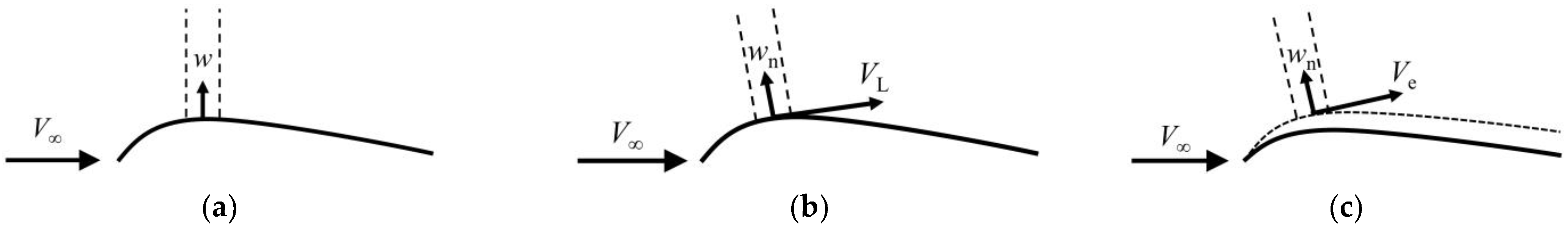
Figure 2.
The local coordinate system .
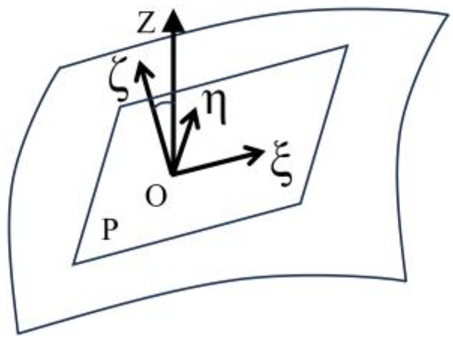
Figure 3.
Mismatched meshes of different interfaces.

Figure 4.
Scheme of the state-space flutter analysis using LPT/VLPT.

Figure 5.
Scheme of the state-space flutter analysis using the mode tracking algorithm.

Figure 6.
Test fin: (a) Configuration; and (b) dimensions.

Figure 7.
Ground vibration test.
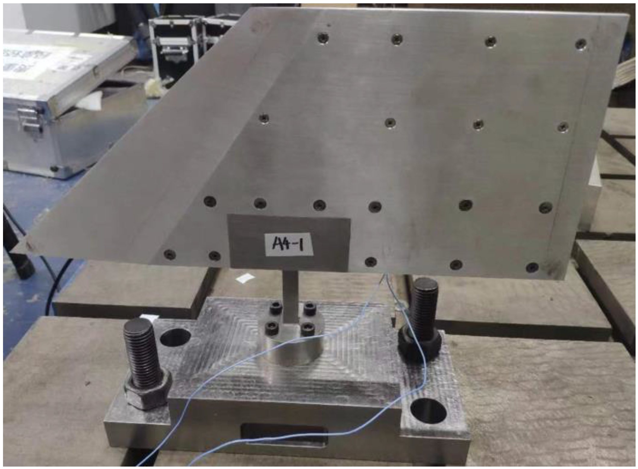
Figure 8.
Wind tunnel test: (a) Wind tunnel layout; and (b) photograph of the scene.
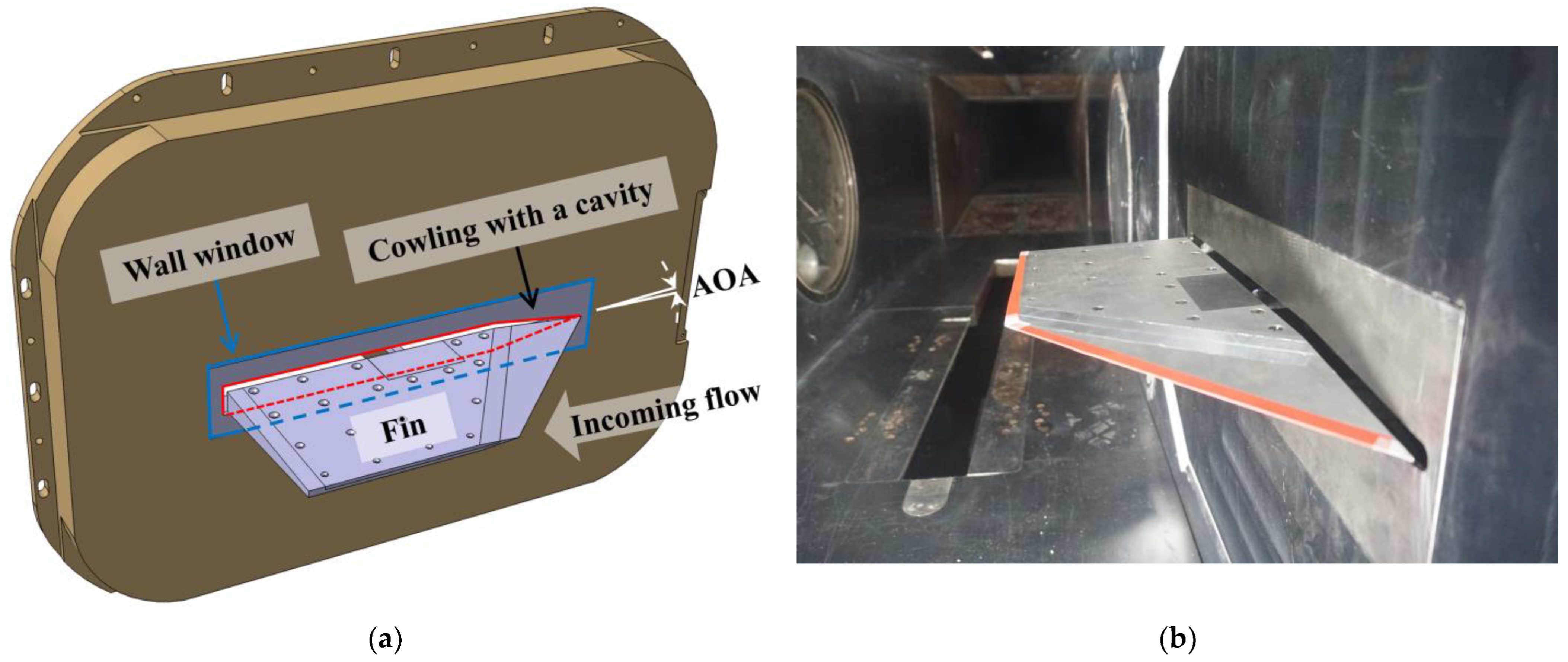
Figure 9.
Computational domain and surface mesh of the CFD model.
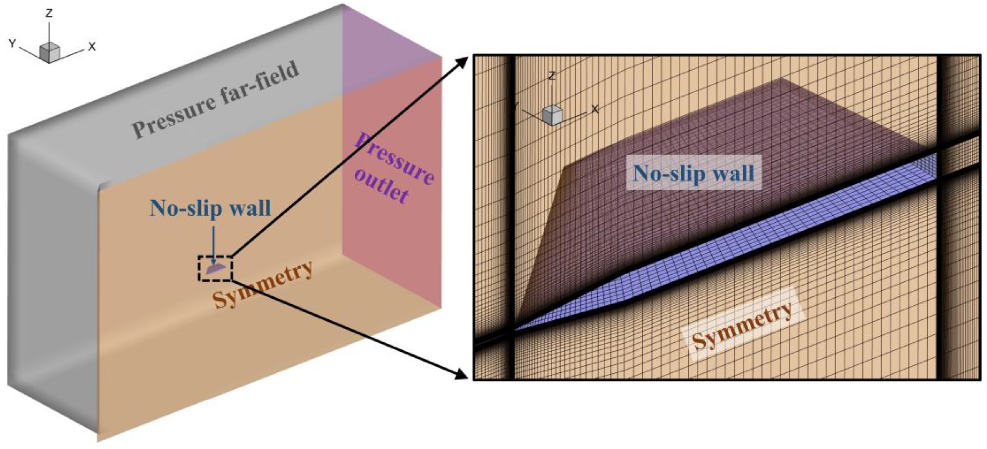
Figure 10.
Effective shape and displacement thickness of VLPT.

Figure 11.
Variation in the displacement thickness of the effective shape changes with the AOA.
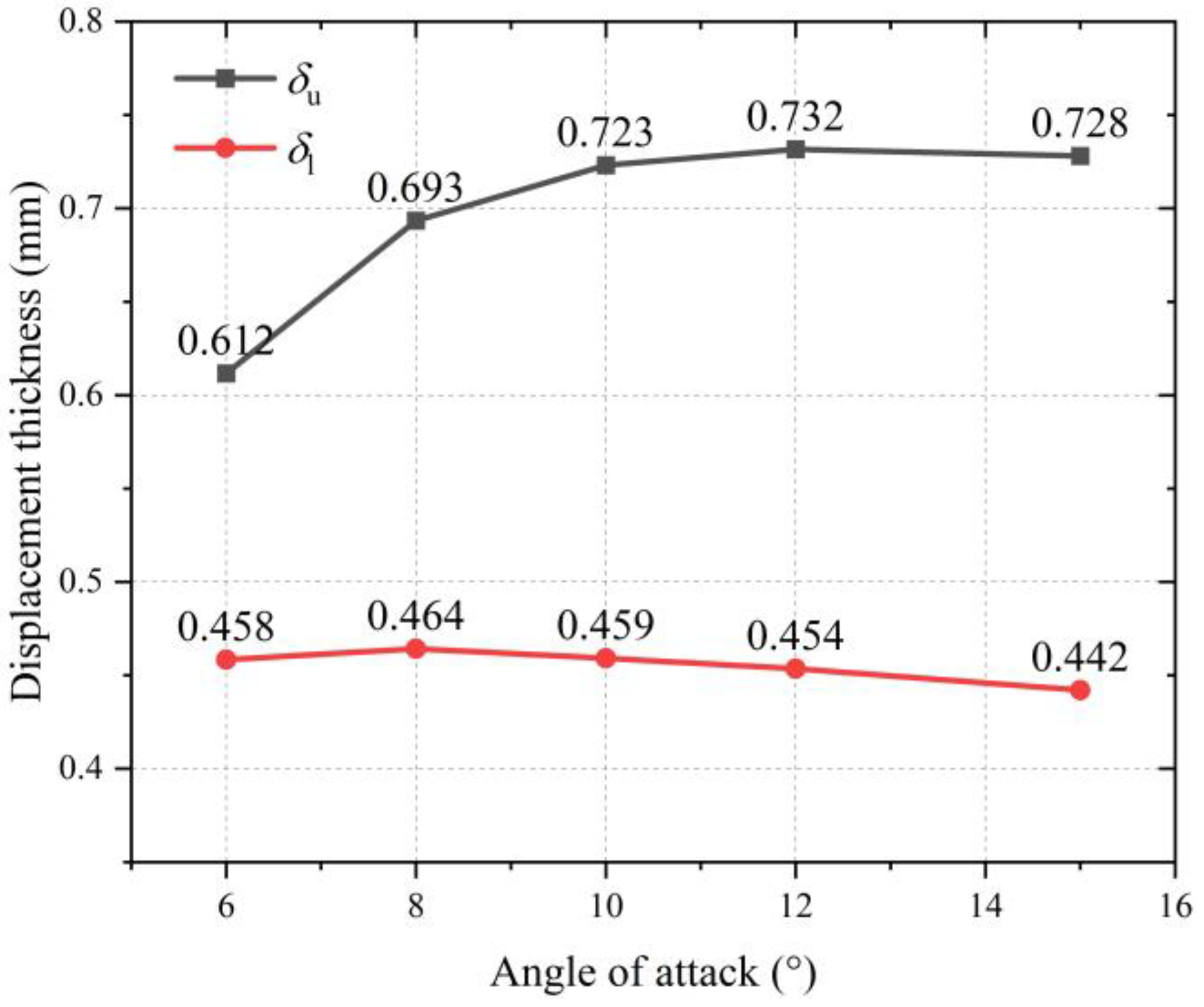
Figure 12.
Pressure distributions of VLPT along the root chord at different AOAs.

Figure 13.
Steady flow fields of VLPT at different AOAs: (a) Pressure distributions and streamlines on the trailing edge section; and (b) streamlines on the upper surface of the fin.
Figure 13.
Steady flow fields of VLPT at different AOAs: (a) Pressure distributions and streamlines on the trailing edge section; and (b) streamlines on the upper surface of the fin.
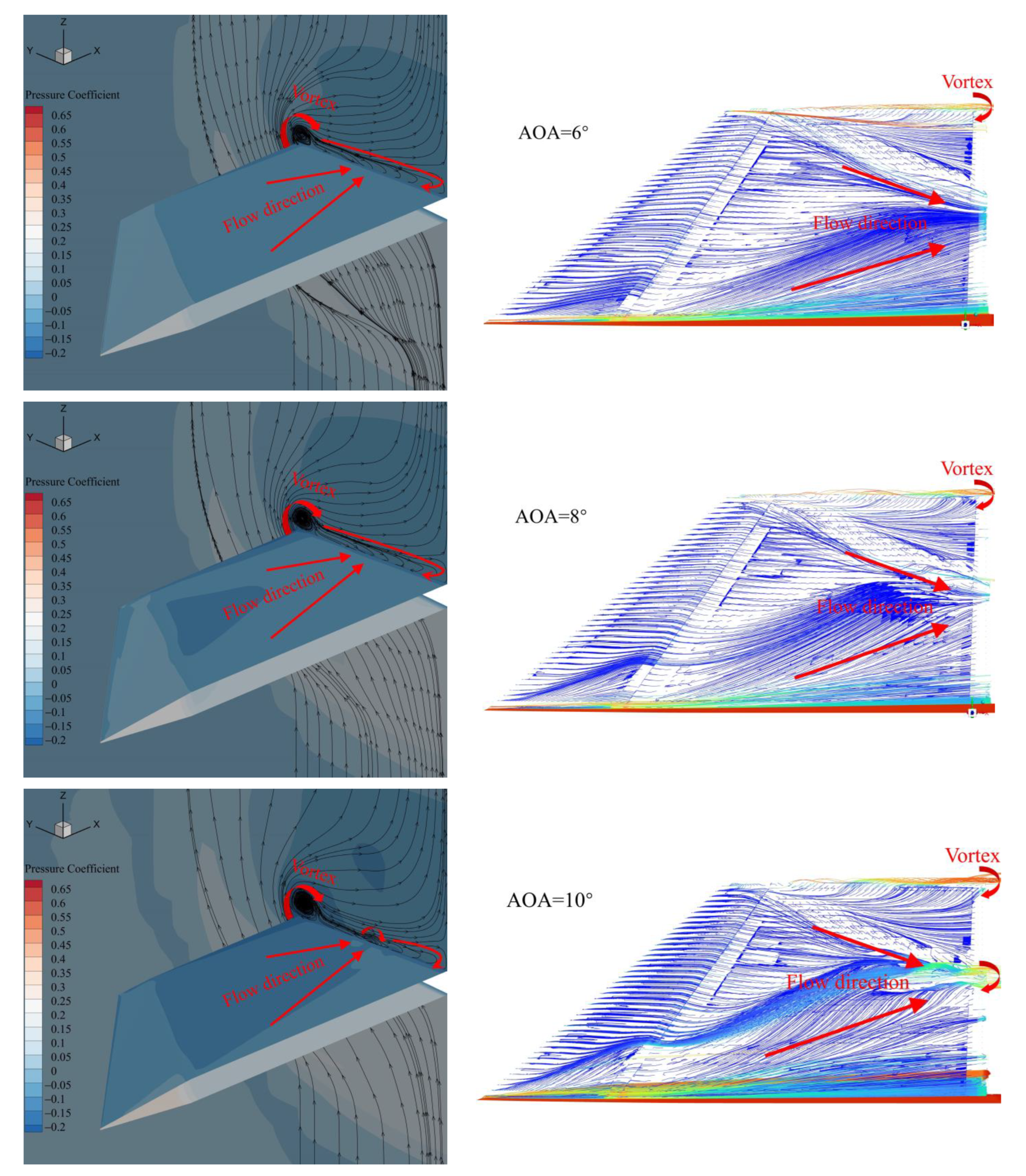
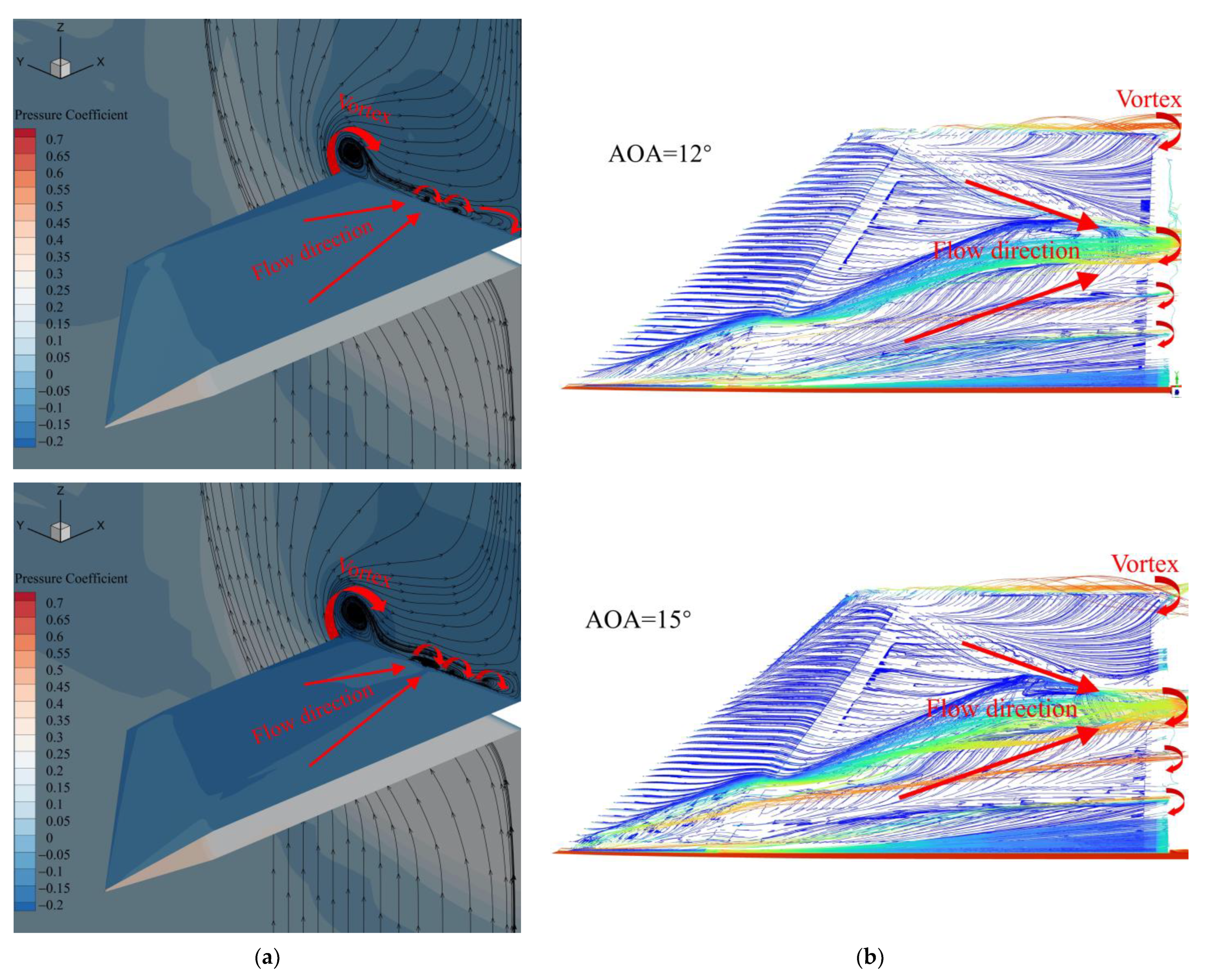
Figure 14.
Flutter diagrams for an AOA of 10° using VLPT: (a) Root locus diagram; (b) V-G diagram; and (c) V-F diagram.
Figure 14.
Flutter diagrams for an AOA of 10° using VLPT: (a) Root locus diagram; (b) V-G diagram; and (c) V-F diagram.

Figure 15.
Flutter comparisons of different methods: (a) Comparison of the flutter speed; and (b) comparison of the flutter frequency.
Figure 15.
Flutter comparisons of different methods: (a) Comparison of the flutter speed; and (b) comparison of the flutter frequency.
Figure 16.
Steady flow fields (pressure distributions and streamlines on the trailing edge section) of LPT: (a) AOA = 6°; and (b) AOA = 15°.
Figure 16.
Steady flow fields (pressure distributions and streamlines on the trailing edge section) of LPT: (a) AOA = 6°; and (b) AOA = 15°.

Table 1.
Mass properties of the test fin.
| Mass (kg) | Center of Mass (mm) | |
|---|---|---|
| X Direction | Y Direction | |
| 2.096 | 14.13 | 26.67 |
Table 2.
Modal properties of the test fin and FE model.
| Order | Frequency (Hz) (Error) | Modal Shape | |
|---|---|---|---|
| Test Model | FE Model | ||
| First torsion | 48.8 | 48.86 (0.12%) |  |
| First bending | 67.8 | 67.77 (−0.04%) |  |
Table 3.
Flutter results of the wind tunnel test.
| AOA (°) | Flutter Dynamic Pressure (kPa) | Equivalent Flutter Speed (m/s) | Flutter Frequency (Hz) |
|---|---|---|---|
| 6 | 71.57 | 341.84 | 59.03 |
| 8 | 68.64 | 334.76 | 59.30 |
| 10 | 67.10 | 330.98 | 58.55 |
| 12 | 67.55 | 332.10 | 59.24 |
| 15 | 66.31 | 329.03 | 59.16 |
Table 4.
Grid independence of three mesh models.
| Mesh Model | Cell Number (Error) | Coefficient (Error) | |
|---|---|---|---|
| Lift | Pitching Moment | ||
| Coarse | 631,056 (26.48%) | 0.2742 (0.36%) | −0.01774 (3.58%) |
| Baseline | 2,383,356 | 0.2733 | −0.01713 |
| Fine | 9,330,400 (391.48%) | 0.2728 (−0.15%) | −0.01690 (−1.34%) |
Table 5.
Flutter results and relative errors of VLPT.
| AOA (°) | Flutter Dynamic Pressure (kPa) | Equivalent Flutter Speed (m/s) | Flutter Frequency (Hz) |
|---|---|---|---|
| 6 | 71.82 (0.35%) | 342.43 (0.17%) | 59.34 (0.53%) |
| 8 | 71.56 (4.25%) | 341.81 (2.10%) | 59.31 (0.02%) |
| 10 | 71.03 (5.86%) | 340.54 (2.89%) | 59.32 (1.32%) |
| 12 | 70.71 (4.68%) | 339.77 (2.31%) | 59.35 (0.19%) |
| 15 | 69.79 (5.25%) | 337.55 (2.59%) | 59.43 (0.46%) |
Table 6.
Flutter results and relative errors of LPT.
| AOA (°) | Flutter Dynamic Pressure (kPa) | Equivalent Flutter Speed (m/s) | Flutter Frequency (Hz) |
|---|---|---|---|
| 6 | 72.28 (0.99%) | 343.52 (0.49%) | 59.34 (0.53%) |
| 8 | 72.27 (5.29%) | 343.50 (2.61%) | 59.38 (0.13%) |
| 10 | 72.19 (7.59%) | 343.31 (3.72%) | 59.44 (1.52%) |
| 12 | 71.99 (6.57%) | 342.83 (3.23%) | 59.51 (0.46%) |
| 15 | 71.65 (8.05%) | 342.02 (3.95%) | 59.65 (0.83%) |
Disclaimer/Publisher’s Note: The statements, opinions and data contained in all publications are solely those of the individual author(s) and contributor(s) and not of MDPI and/or the editor(s). MDPI and/or the editor(s) disclaim responsibility for any injury to people or property resulting from any ideas, methods, instructions or products referred to in the content. |
© 2023 by the authors. Licensee MDPI, Basel, Switzerland. This article is an open access article distributed under the terms and conditions of the Creative Commons Attribution (CC BY) license (https://creativecommons.org/licenses/by/4.0/).
Share and Cite
MDPI and ACS Style
Liu, C.; Xie, C.; Meng, Y.; Bai, L. Experimental and Numerical Flutter Analysis Using Local Piston Theory with Viscous Correction. Aerospace 2023, 10, 870. https://doi.org/10.3390/aerospace10100870
AMA Style
Liu C, Xie C, Meng Y, Bai L. Experimental and Numerical Flutter Analysis Using Local Piston Theory with Viscous Correction. Aerospace. 2023; 10(10):870. https://doi.org/10.3390/aerospace10100870
Chicago/Turabian StyleLiu, Chenyu, Changchuan Xie, Yang Meng, and Liuyue Bai. 2023. "Experimental and Numerical Flutter Analysis Using Local Piston Theory with Viscous Correction" Aerospace 10, no. 10: 870. https://doi.org/10.3390/aerospace10100870
Note that from the first issue of 2016, this journal uses article numbers instead of page numbers. See further details here.