
Multiscale Aeroelastic Optimization Method for Wing Structure and Material

1
School of Aeronautic Science and Engineering, Beihang University, Beijing 100191, China
2
Institute of Unmanned System, Beihang University, Beijing 100191, China
*
Author to whom correspondence should be addressed.
Aerospace 2023, 10(10), 866; https://doi.org/10.3390/aerospace10100866
Submission received: 11 September 2023
/
Revised: 26 September 2023
/
Accepted: 30 September 2023
/
Published: 2 October 2023
(This article belongs to the Special Issue Advanced Aircraft Technology)
Abstract
:Microstructured materials, characterized by their lower weight and multifunctionality, have great application prospects in the aerospace field. Optimization methods play a pivotal role in enhancing the design efficiency of both macrostructural and microstructural topology (MMT) for aircraft. This paper proposes a multiscale aeroelastic optimization method for wing structure and material considering realistic aerodynamic loads for large aspect ratio wings with significant aeroelastic effects. The aerodynamic forces are calculated by potential flow theory and the aeroelastic equilibrium equations are solved through finite element method. The parallel design of the wing MMT is achieved by utilizing the optimization criterion (OC) method based on sensitivity information. The optimization results indicate that wing elastic effects reinforce the outer section of the wing structure compared with the optimization results obtained under rigid aerodynamic forces. As the optimization constraints become more rigorous, the optimization results show that the components with larger loads are strengthened. Furthermore, the method presented in this paper can effectively optimize the wing structure under complex boundary conditions to achieve a reasonable stiffness distribution in the wing.
1. Introduction
Long-endurance vehicles typically use wings with large aspect ratios to achieve superior aerodynamic performance. The wings undergo considerable bending and torsional deformation due to aerodynamic force, resulting in significant aeroelastic effects [1]. In aircraft design, traditional design methods tend to introduce the undertaking of load analysis and the consideration of aeroelasticity effects on the aircraft late in the design process, leading to increased mechanical mass, reduced aerodynamic performance, and wasted resources due to duplicate designs [2]. Therefore, modern design concepts propose fully considering the impact of aeroelasticity during the initial aircraft design stage, maximizing the utilization of structural deformation through optimization methods, and achieving a lighter wing structure. In previous studies, aeroelastic optimization has usually included the design of wing structural stiffness [3], the layout of the aerodynamic shape [4]. With the advancement of computational techniques, topology optimization methods have been widely used in aeroelastic optimization. This more efficient method has become a design tool which aims to improve aircraft performance and reduce weight [5].
Topology optimization methods seek the optimal material layout in the reference domain, in order to satisfy constraints and minimize the objective function. The current topology optimization methods mainly comprise the level-set method (LSM) [6], evolutionary structural optimization (ESO) [7], and solid isotropic material with penalization (SIMP) [8,9]. The LSM provides precise mathematical derivations and a clear description of topological boundaries. Thus it is widely used in academic research [10]. The primary difficulty of the conventional LSM is resolving the “Hamilton–Jacobi equation [11]”. Wang et al. [12] used radial basis functions to interpolate the level-set function. This method is known as the parameterized level-set method (PLSM). By separating the temporal and spatial terms in the level-set function, the partial differential equations (PDEs) in optimal control are transformed into ordinary differential equations. The PLSM has the advantage of being both efficient and accurate.
Optimizing structural topology has the potential to enhance mechanical properties [13]. Based on this concept, researchers have considered designing microstructural topology on the microscopic scale to optimize material properties. Macrostructural topology is formed by stacking and mixing microstructured material to achieve an overall structure with superior properties [14]. Rodrigues [15] pioneered the optimization of structural performance by considering both “structure” and “material”. The first step is to design the macrostructure, followed by optimizing the topological shape of the microstructured material using the density of each finite element as the objective. Jie Gao et al. [16] investigated the issue of multiscale topology optimization for 2D and 3D structures and materials. They utilized SIMP with compliance as the objective function to obtain MMT and provided their concise and efficient Matlab code. The characteristics of microstructured material align well with the rigorous quality requirements of the aerospace industry, leading scientists to explore their potential use in aircraft. An example of this is the work performed by Cramer et al. [17], who utilized an octahedral-shaped microstructured material to create the internal structure of a flexible vehicle. As a result, this vehicle’s mass density was found to be lower than that of a bird-like vehicle. Microstructured material has also been used in commercial aircraft wing structures [18] and hypersonic applications [19], demonstrating favorable characteristics. In addition, Jenett et al. [20] designed two different microstructural topologies, aligned along the span and chord directions of the wing, to realize the stiffness design of the wing. They also performed an aeroelastic analysis. Nevertheless, the microstructural topology is based on empirical design and a fixed topology does not fully exploit the properties of the microstructure material. Wang et al. [21] applied multiscale topology optimization to tackle the internal structure design issue of the hypersonic vehicle rudder in aerospace. They used the SIMP to obtain a hybrid structure with specific stiffness exceeding that of the solid structure. However, the boundary conditions in the study simplify the flight load to a uniformly distributed aerodynamic pressure, which does not accurately reflect the realistic load experienced by the vehicle during flight.
Optimization methods have significant potential to increase the design efficiency of MMT in aircraft. However, the aerodynamic load distribution of the aircraft during flight is complex. The simplified boundary conditions of the optimization make difficulties in applying the designed MMT. This paper presents a method for multiscale aeroelastic optimization of the wing structure and material, in which both rigid and elastic aerodynamic forces are considered separately for the boundary conditions of the optimization problem to investigate the influence of elastic effects. The linearized aerodynamic potential flow theory is used to calculate the rigid aerodynamic forces, and static aeroelastic response equations are employed to calculate the elastic aerodynamic forces. The response equations are solved using finite element method. The MMT is described using the PLSM, and the equivalent elasticity matrix is calculated through the homogenization method, which is then combined with the macrostructure topology to obtain the stiffness matrix. Sensitivity calculations for the optimization problem are performed using numerical methods. The optimization criterion method is used to iterate the design variables, enabling parallel design of the wing’s MMT.
2. Methods
2.1. Homogenization Method
For microstructured material, analyzing boundary problems with a large number of microstructural components is time-consuming and difficult. As a solution, the mechanical properties of these materials are often replaced with an equivalent material model. This process, known as homogenization, is commonly used to simplify analysis [22]. From a mathematical perspective, the theory of homogenization can be viewed as a limit theory that uses asymptotic expansion and the assumption of periodicity to substitute differential equations that have rapidly oscillating coefficients with differential equations whose coefficients are constant or slowly varying in such a way that the solutions are close to the initial equations. Homogenization theory requires two conditions: (1) the microstructure must be significantly smaller than the entire spatial domain, and (2) the material must have a periodic arrangement of the microstructure. To describe all quantities within a microstructured material, two coordinate systems are employed: one on the macroscopic or global coordinates (x), which indicates slow variations, and the other on the microscopic or local coordinates (y), which describes rapid oscillations. Consequently, the displacement field in the macroscopic material can be expressed through the two-scale asymptotic expansion of the theory:
where ε is a small parameter that indicates the ratio between the length of a unit vector in microscopic coordinates and the length of a unit vector in macroscopic coordinates.
According to the principle of virtual work and incorporating (1), the equivalent elastic tensor of the lattice material can be expressed by considering only the first-order expansion terms of the parameters:
where is defined as the area (2D) or volume (3D) of the microstructure, and corresponds to the initial unit test strain fields, and and represent the response strain of the microstructure, which is solved using the elastic balance equation:
where vi is defined as virtual displacement. To solve equation, the microstructure is imposed with the unit test strain fields and the periodicity condition is satisfied [23]. Consequently, the displacement field can be expressed as follows:
where is the periodic fluctuation displacement field. This field is unknown and difficult to solve. Hence, Equation (4) is transformed by the displacement constraint relation satisfied by the corresponding points on the symmetric boundary:
where denotes the length between corresponding points on the symmetric boundary of the microstructure. According to (5), the boundary constraint equations of the microstructure can be added directly. In addition, Equation (5) makes it possible to reduce the linear elastic equilibrium equations and speed up the computational efficiency of finite elements [24].
2.2. Parameterized Level-Set Methods
An LSM is an implicit method for describing structural boundaries [25]. The surface is represented implicitly through a level-set function Φ(x), which is Lipschitz-continuous, and the surface itself is the zero isosurface or zero level-set . In the present level-set-based shape and topology optimization method, the shape and topology of a structure are described by a level-set function Φ(x) defined as:
where is a fixed reference domain in which all admissible shapes Ω (a smooth bounded open set) are included. Γ is denoted as the boundary of the structural topology with level-set function of size 0.
Furthermore, the surface motion can be described by PDEs involving Φ(x). The normal velocity V is used as the advection velocity in the following Hamilton–Jacobi equation:
where t represents the pseudo time of the optimization. Therefore, the direction and distance of the shape boundary movement can be determined by solving Equation (7). However, obtaining analytical solutions for PDEs are difficult. In a Eulerian approach, a numerical procedure for solving the Hamilton–Jacobi PDEs are indispensable. This procedure requires an appropriate choice of upwind schemes, extension velocities and reinitialization algorithms, which may limit the utility of the LSM. In order to solve the above problems, an interpolation function is employed to enhance the accuracy and effectiveness of the LSM. In this work, the compactly supported radial basis function (CSRBF), as presented by Wendland, is adopted [26]:
where r is the radius of support defined in a two-dimensional Euclidean space, as:
where dI denotes the Euclidean distance between the current sample knot and the knot within the whole reference domain. The parameter dmI defines the size of the influence domain of the sample knot. The level-set function is obtained by using a series of CSRBFs with interpolation of N different knots. The parameterized level-set function is denoted as [27]:
where αi is the expansion coefficients of the CSRBF at the ith knot, which is only dependent on time. Thus, (10) can be expressed in the form of a matrix:
where:
The topological control equations based on the CSRBF function can be obtained by bringing the parameterized level-set into Equation (7):
The decoupling of the temporal and spatial terms can be realized through the PLSM. In addition, the time-varying initial value problem is transformed into a relatively simple generalized expansion coefficient initial value interpolation problem. This can greatly improve the optimization efficiency [28].
2.3. Multiscale Aeroelastic Optimization Method for Wing Structure and Material
Mass is a crucial factor in evaluating the performance of a flying vehicle. Topology optimization proves to be an efficient method, enabling the vehicle to fulfill the stiffness requirement while reducing its weight. The aerodynamic loading on a large aspect ratio wing leads to a significant aeroelastic effect. The distribution of aerodynamic loads is influenced by the elastic effect. Therefore, it is necessary to consider the influence of the elastic effect in the multiscale optimization problem of aircraft wings’ structure and material.
In this paper, a multiscale aeroelastic optimization method is established for large aspect ratio wings. The optimization framework is depicted in Figure 1 and consists of three primary steps: finite element model updating, aeroelastic analysis, and optimization iteration.
Finite element model updating occurs in two steps. First, the equivalent elasticity matrix of the microstructured material is computed using the homogenization method based on the microstructure level-set function. Second, the stiffness matrix of the overall structure is obtained based on the level set function of the macrostructure. The mechanical properties of the material are defined by employing the previously obtained equivalent elasticity matrix. For aeroelastic analysis, the linearized aerodynamic potential flow theory is utilized to determine the rigid aerodynamic forces. The static aeroelastic response equations are solved to obtain the elastic aerodynamic force and elastic deformation. From the aeroelastic analysis results, the values for the objective and constraint functions can be determined. Optimization iterations begin with a numerical method to obtain the sensitivity values of the objective and constraint functions to the macro and micro design variables. Next, the OC method is used to iterate the design variables and finally the optimization is stopped until the convergence condition is satisfied.
2.3.1. Macro- and Microstructure Design Variables
The structural and material optimization problem is divided into two problems according to scale. The microscopic scale is used in designing the topology of the microstructure. Different microstructural topologies produce different equivalent elastic matrices and therefore have an impact on the overall stiffness. The macroscopic scale is used in designing the topology of the overall structure and is analogous to traditional structural topology optimization. By filling the reference domain with materials to form a more efficient structure, better objective performance is achieved. The macroscopic scale of the multiscale optimization problem determines the overall structure and defines the existence of microstructure. The microscopic scale determines the microstructural topology and governs the equivalent properties of the microstructured material. During the optimization process, the MMT is iterated simultaneously to approximate optimal objective performance.
The objective of multiscale optimization includes both macrostructural and microstructural topology. Thus, it is necessary to define multiple level-set functions that describe the topology of these structures. The level-set functions are represented as follows:
where ΦM and Φm are the level-set functions of the macrostructural and microstructural topology, respectively. ΩM, ΓM, and DM represent the design domain, structural boundaries, and reference domain of the macrostructure. Ωm, Γm, and Dm represent the design domain, structural boundaries, and reference domain of the microstructure.
The level-set functions are interpolated for the MMT using CSRBFs. The parameterized level-set is interpolated in the following form:
where and represent the CSRBFs and the expansion coefficients of the macrostructure, respectively. and represent the CSRBFs and the expansion coefficients of the microstructure, respectively. The N and n interpolation points have been selected for the macro and micro level-set functions, respectively.
2.3.2. Optimization Model
For static stiffness design, the problem of topology optimization can be described as minimizing the compliance of the structure under a given load, where both the macrostructure and microstructure satisfy the volume constraints. Thus, the minimum compliance problem, which is based on parameterized level-sets, can be expressed as the following mathematical model:
where J represents compliance, which is used as the optimization objective in this paper. GM(ΦM) and Gm(Φm) represent the volume constraints of the macrostructure and microstructure, respectively. The maximum volume allowed in the optimization are indicated by VM, Vm, , and are the expansion coefficients, which are used as design variables. uM and um are the displacement fields for the macrostructure and microstructure, respectively. vM and vm represent the virtual displacement fields. EH refers to the equivalent elastic tensor. The heaviside function H(ΦM) is determined by the level-set function and signifies the presence of material at each point. Equations for linear elastic equilibrium are written in a weakly solved form based on the energy bilinear form a(ΦM, uM, vM, EH) as well as the load linear form l(ΦM, vM). The specific forms are defined as:
where fM and pM represent the body and surface forces, respectively.
The static problem involves constant body and surface forces, resulting in constant boundary conditions throughout the optimization process. In contrast, the aeroelastic optimization problem involves the elastic deformation of the wing structure due to aerodynamic forces, resulting in the redistribution of aerodynamic forces. As the volume constraint decreases, reducing wing stiffness, the elastic effect becomes increasingly pronounced, resulting in a significant distinction between the elastic and rigid aerodynamic forces. The boundary conditions of the optimization problem under realistic flight loads are constantly changing. Equation (18) is transformed into finite element form based on the principle of virtual work. The linear elastic equilibrium equations are expressed under flight loads as:
where K is the stiffness matrix of the structure, FI represents the inertial force load vector, which is generated by the acceleration of the rigid body motion, FA represents the aerodynamic force load vector. The aerodynamic loads include rigid aerodynamic forces and additional aerodynamic forces caused by the elastic deformation of the structure. Hence, according to Equation (19), the static aerodynamic elastic response equation of the aircraft can be obtained as:
where represents the aerodynamic forces caused by the elastic deformation of the structure, represents the aerodynamic forces generated by flight parameters such as the angle or rudder deflection. By solving (20) using finite element method, flight parameters, structural deformation, and elastic aerodynamic force distribution can be obtained.
Rigid aerodynamic computational methods for aeroelastic analysis can be categorized into linear and nonlinear methods. Among these, the surface element method, based on the linearized aerodynamic potential flow theory, is suitable for optimization problems and enables quick calculation of the rigid aerodynamic loads. It follows a specific format:
where is defined as the Mach number and φ represents the perturbation velocity potential. Equation (21) is solved with the doublet-lattice method (DLM), which considers the wing as a plane and divides the mesh. Different fundamental solutions are defined in each mesh and results are obtained for the velocity potential based on the boundary conditions. The velocity potential provides the perturbed velocity, which is then used to solve the pressure distribution through Bernoulli’s equation.
2.3.3. Sensitivity Analysis
In aeroelastic optimization, the first-order derivatives of the objective with respect to the macroscopic expansion coefficients are computed by using the shape derivative, stated as [29,30]:
where δ(ΦM) is the partial derivative of the Heaviside function, namely the Dirac delta function. The specific form of β(uM, EH) is as follows:
Similarly, the first-order derivative of the macroscopic volume constraint with respect to the macroscopic expansion coefficients can be computed in the following form:
The first-order derivative of the objective function with respect to the microscopic expansion coefficients is
where is the first-order derivative of the equivalent elasticity tensor with respect to microscopic expansion coefficients in the following form:
Similarly, the first-order derivatives of the microscopic volume constraint with respect to microscopic expansion coefficients can be computed in the following form:
Here, the OC algorithm is used to update the design variables in the multiscale design. The details for updating the mechanism in the OC method are described in [31]. The update scheme for the microscopic expansion coefficients is shown below:
where represents the value of the ith expansion coefficient of the macrostructure in the (k+1)th step. represents the move limit of the macroscopic design variable, which determines the limit of variation in the level set function. is the damping factor. is the updating factor of the ith design variable of the macrostructure in the kth step, which is denoted as:
where μ is a small value, in order to avoid an updating factor denominator of 0. is the lagrange coefficient of the kth step of the macrostructure. Similarly, an updated iteration scheme for the microscopic expansion coefficients can be obtained.
3. Results
3.1. Cantilever Beam
In this example, the cantilever beam is used to study the efficiency of the proposed multiscale topology optimization method. As displayed in Figure 2, the reference domain for the macrostructure is a rectangular area measuring 100 mm × 50 mm, whereas the reference domain for the microstructure is a square area measuring 1 mm × 1 mm. The left side of the beam has a fixed boundary condition, whereas the right side is subjected to symmetrical load. Steel, with a modulus of elasticity of 7.1 × 10⁴ MPa and Poisson’s ratio of 0.33, is selected as the material for the microstructure.
This example is based on an optimization problem with fixed loads. The objective function is used to minimize the compliance of the structure. The maximum volume constraints VM and Vm are defined as 40% and 30%, respectively. The macrostructure is discretized using 1 × 1 four-node rectangular finite elements, and 0.02 × 0.02 finite elements are used to discretize the microstructures. In the OC method, the move limits and are 0.01 and 0.005, respectively, with a damping factor of 0.3. Macrostructures and microstructures reach the volume constraints after 100 steps.
In addition, the traditional PLSM is utilized to optimize the cantilever beam structure and investigate the similarities and differences between single-scale and multiscale optimization. For single-scale optimization, a volume constraint of 0.12 is imposed to maintain the same mass as multiscale optimization.
The iterations of the objective functions and constraints are displayed in Figure 3. The blue line illustrates the convergence process of the multiscale optimization, and the red line illustrates the convergence process of the single-scale optimization. Figure 3a shows that the multiscale topology optimization requires more steps for convergence than the single-scale topology optimization due to the greater number of design variables. In the first 100 steps of optimization, the objective functions gradually increase as the volume constraints decrease. Once these 100 steps are completed, the volume constraints maintain a constant value, while the objective gradually decreases throughout the iteration. It should be noted that the stiffness of the single-scale topology is greater than that of the multiscale topology for the same mass. It is shown that the stiffness properties of a single type of microstructured material are not as good as those of solid materials, and this conclusion is consistent with the results of [32]. Figure 3b shows the macrostructural volume (MAV) and microstructural volume (MIV) for multiscale optimization as well as the structural volume (MV) for single-scale optimization. The results show that the mass of both multiscale and single-scale optimized structures are significantly reduced in comparison with that of the initial structure.
The optimization results at different steps are demonstrated in Figure 4 and Figure 5, with both multiscale and single-scale methods used. Results indicate similar trends in the optimization iterations for both macrostructures. The final structure exhibits a truss-like design with a thicker top and bottom, and a middle section formed by a connected beam-like structure. The final masses for multiscale and single-scale optimization are equivalent. The multiscale optimization employs less dense microstructured material, resulting in a larger macro volume.
The optimized microstructural topology features two thicker beam-like structures in the X-direction and connects the Y-direction through four rods located at the top and bottom.
The optimized cantilever beam is shown in Figure 6, where the macrostructure consists of microstructured materials.
The stress distribution of the structures obtained through single-scale and multiscale optimization are shown in Figure 7. Shear forces and bending moments act on the cantilever beams, with the upper and lower side beams primarily bearing the tensile and compressive stresses created by the bending moments. These stresses are then transferred to the fixed boundary. In terms of stress levels, the structure experiences significantly lower stress magnitudes when subjected to multiscale optimization in comparison with single-scale optimization. This is demonstrated by the fact that microstructured material can significantly decrease the stress values of a structure, even though it has decreased stiffness properties.
3.2. Multiscale Optimization of Structure and Materials for Wings with Large Aspect Ratios
In this section, the wing of a large aspect ratio aircraft is selected as the object of study, and the model refers to the Global Hawk Unmanned Aerial Vehicle (UAV) [33]. The geometric parameters are presented in Figure 8 with LRN1015 selected as the airfoil of the wing. The half wingspan length is 14.39 m, the wing root chord length is 1.52 m, and the leading edge sweep-back angle is 5.9°. The wing box segment highlighted in green is the reference domain for topology optimization. Different materials are utilized for the skin and internal structure of the wing box. The skin is made of composite material, which mainly maintains the aerodynamic shape of the wing. The internal structure is constructed of a singular microstructured material. Titanium alloy with a modulus of elasticity of 1.09 × 10⁵ Mpa and Poisson’s ratio of 0.31 is chosen for the microstructure. During the optimization, the equivalent mechanical properties of the microstructured material are determined by the microstructure topology. The macrostructure is discretized with 3600 hexahedral elements. The reference domain for microstructure measures 20 mm × 20 mm × 20 mm and significantly smaller than the macrostructure. It is discretized with eight-node hexahedral elements of 1 mm × 1 mm × 1 mm.
A section of the wing is selected to display the initial model, as shown in Figure 9. The profile features a total of six spherical holes, each with a 5 mm radius. In the internal structure, there are a total of 384 such holes. Therefore, the initial macrostructural volume constraint is 0.972. The initial model of microstructure is entirely filled, resulting in the initial microstructural volume constraint of 1.0.
3.2.1. Multiscale Aeroelastic Optimization of Wing Structure and Material under Rigid and Elastic Loading
Here, the proposed method is applied to topologically design a wing with a large aspect ratio through both macrostructural and microstructural parts. The flight speed corresponds to 0.785 Ma at an altitude of 15,000 m and the dynamic pressure is 3051 Pa. The flight angle is 4°. The optimization problem has a macrostructural volume constraint of 0.7 and a microstructural volume constraint of 0.7. In the OC method, the move limits and are 0.002 and 0.05, respectively, with a damping factor of 0.3. The optimization objective is to minimize the compliance of the wing structure. Two boundary conditions for loading are used: elastic and rigid loads. The elastic load considers the effects of elasticity on the aerodynamic force.
The objective functions and the iteration process of the MMT constraints are shown in Figure 10. The first 100 steps decrease the structural stiffness as the volume of the MMT decreases. This leads to an increase in compliance. Once the volume constraints are reached, the compliance gradually decreases. Optimal results for the two distinct boundary conditions are larger for the elastic loading than for the rigid loading. Since the constraint iteration process of the optimization problem under elastic and rigid loading is approximated, the convergence process of the MMT constraints can be represented by the two blue lines. The volume constraints reach the constraints after 100 steps for both the MMT and remains constant.
The aerodynamic force distributions, both elastic and rigid, are presented in Figure 11. It can be observed that the aerodynamic forces, regardless of being elastic or rigid, follow a similar trend along the spanwise direction of the wing. Moreover, the aerodynamic bending moments and shear forces increase from the wing tip to the wing root, and the maximum aerodynamic load is at the wing root. The elastic aerodynamic forces resulting from wing structure deformation are illustrated in Figure 12. Due to the UAV wing’s small sweep-back angle and the outer section’s lower stiffness compared with the inner section, the outer section generates a larger positive torsion under aerodynamic force, thereby increasing the aerodynamic force. It is noteworthy that the elastic aerodynamic force surpasses the rigid aerodynamic force for identical angles, leading to relatively larger optimization results when the elastic effect is taken into account.
The optimized density of elements for the final macrostructure under rigid and elastic boundary conditions is shown in Figure 13. The reference domain is partitioned into five color fields based on the density of elements, with the red region approaching a density of 1.0 and the blue region approaching a density of 0.0. Due to the similarity in load distribution along the wing’s spanwise direction under rigid and elastic aerodynamic forces, the trends in the density of elements exhibit three characteristics: (1) a gradual decrease in density from the wing’s root to its tip, (2) larger density of elements in the upper and lower portions than in the middle portion, and (3) a larger density at the wing box’s front end compared with the density at its back end. Specifically, a density value of 1.0 is distributed primarily at the upper and lower parts of the wing root’s front end. When elastic effects are considered, the density value of elements in the wing’s outer section increases.
The optimized macrostructural topology is displayed in Figure 14a. The red region has a density interval of 0.6–1.0, while the green region has a density of 0.2–0.6, and the blue region has a density of 0.0–0.2. During the solving of static aerodynamic elastic response equation, the density of elements in the macrostructure establishes a threshold value of 0.001. This ensures that the stiffness matrix is nonsingular. However, the display of macrostructural topology does not incorporate the threshold density. Due to the lower load on the outer section of the wing compared to the inner section, the optimization process significantly reduced the structure of the outer section of the wing.
To achieve a macrostructural topology that is useful for engineering realization, this paper conducts a post-processing of the optimized outer segment structure of the wing. Macrostructural elements with wing span positions greater than 11,500 mm were selected and their densities averaged to the designated structural elements on the outside of the wing. The results are shown in Figure 14b.
The compliance of the structure obtained by optimization and post-processing is shown in the Table 1. The objective of the post-processed structure is 11% larger than the optimization structure. The following sections of this paper will outline the post-processing structure, resulting in a more definitive macrostructural topology.
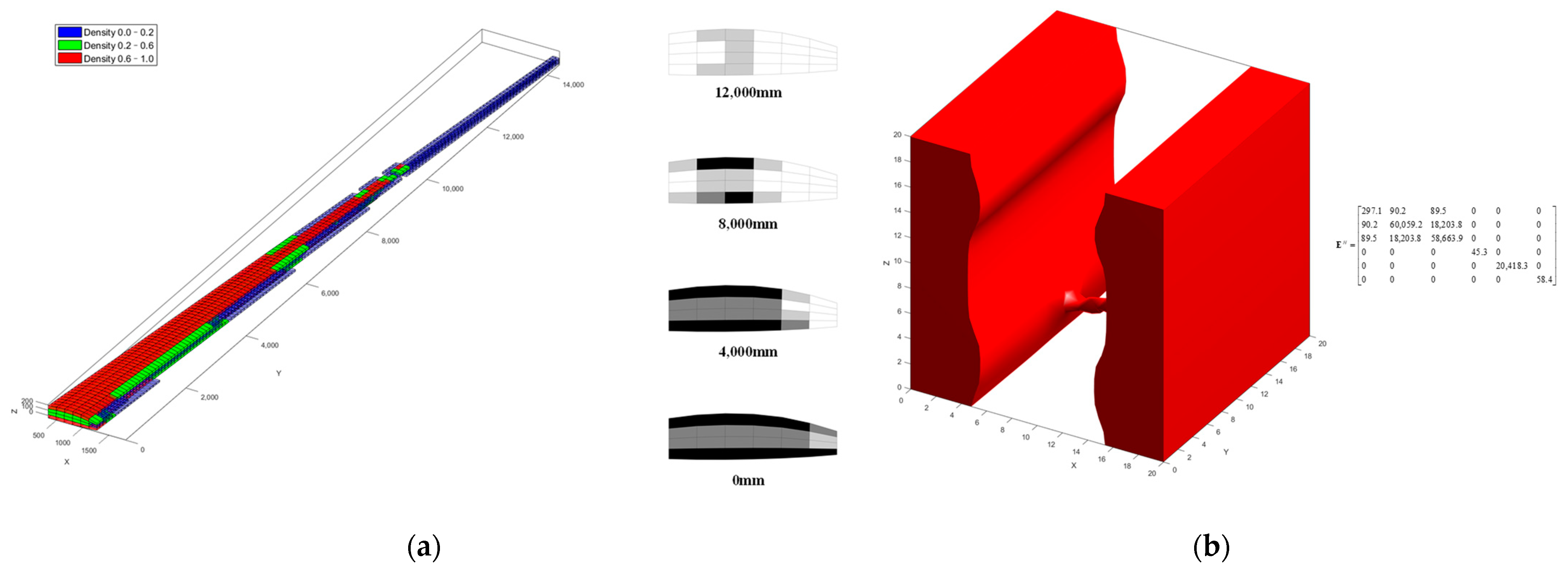
The optimized MMT is displayed in Figure 14, Figure 15 and Figure 16. Results from the optimization problem with two boundary conditions show similar topological. On the macroscopic scale, the wing structure decreases gradually along the Y-direction with the wing root maintaining a more complete structure. Along the Z-direction, the middle region displays a more pronounced weakening, resulting overall in a flanged beam structure. On a microscopic scale, a cylindrical hole is cut out at the center of the square’s structural reference domain along the Y-axis. The elastic matrix of the micromaterial structure demonstrate that the modulus is smaller along the X-axis than in other directions.
Through load analysis, it becomes apparent that the load on the wings outer section is minimal. Consequently, the macrostructure of the optimization problem focuses on weakening the outer section of the structure. The wing structure primarily endures shear force and a bending moment. The shear force causes the wing to require increased stiffness in the Z-direction. Additionally, the bending moment results in the upper and lower portions of the wing structure being subjected to larger tensile and compressive stresses along the Y-direction. Thus, on the macroscopic scale, the optimization problem assigns more structure to the more load-bearing sections, resulting in a layout form similar to the flanged beam. When the sweep-back angle is small, the outer section of the wing experiences positive torsion that results in an increase in aerodynamic forces. Therefore, the optimization outcome under elastic load allocates more structures to the outer section of the wing compared with the rigid load, thus limiting the elastic deformation of the wing. The aeroelastic problem should be considered at the beginning of the vehicle’s stiffness design. The microstructured material will offer more stiffness along the Y and Z directions under aerodynamic loading, which also emanates from the load distribution of the wing.
3.2.2. Multiscale Optimization of Wing Structure and Material with Different Volume Constraints
This section considers the effect of volume constraints on the optimization problem. In an aeroelastic problem, the vehicle is trimmed by accounting for aerodynamic, inertial, and elastic forces. Decreasing the volume constraint will lead to a decrease in the stiffness of the structure. Under loading, the resulting larger bending and torsional deformations have an impact on the aerodynamic loads. The flight conditions in this section align with Section 3.2.1, with a macroscopic volume constraint of 0.4 and a microstructural volume constraint of 0.5.
The wing’s external loads are composed of aerodynamic and inertial forces, distributed as depicted in Figure 17. The MMT volume constraints are 0.7/0.7 abbreviated as Ma_0.7Mi_0.7 and the MMT volume constraints are 0.4/0.5 abbreviated as Ma_0.4Mi_0.5. Load distribution remains constant across different volume constraints. Shear force and bending moment gradually increase from the wing tip to the wing root, with maximum shear force occurring at the wing root. The decrease in volume constraints results in decreased wing structural stiffness, thereby inducing larger elastic aerodynamic force. The flight load for Ma_0.4Mi_0.5 is significantly larger than for Ma_0.7Mi_0.7.
The density distribution of the macrostructure obtained from the optimization problem of Ma_0.4Mi_0.5 is shown in Figure 18a. The overall distribution trend of density is similar to that of the Ma_0.7Mi_0.7 structure. Elements with higher density values are mainly distributed on the upper and lower parts of the wing root. Figure 18b compares the percentage of element volume with total volume at different spanwise stations. In the case of Ma_0.4Mi_0.5, the volume fraction of elements between the 2000 position on the wing span and the wing tip is 61.3%. In Ma_0.7Mi_0.7, the volume fraction is 65.9%. Hence, Ma_0.4Mi_0.5 has a higher percentage of element volume than Ma_0.7Mi_0.7 in the inner section of the wing.
Figure 19 displays the MMT achieved for Ma_0.4Mi_0.5, which still exhibits a structure comparable to that of Ma_0.7Mi_0.7. In addition, cross sections of the optimized macrostructure are given for the four span positions, with the darker shade indicating higher density.
Along the X-direction, the microstructure is reduced, and only a slender rod remains linked to the X-direction. Analysis of the equivalent elasticity matrix of the microstructured material indicates that the modulus is greater in the Y- and Z-directions, but smaller in the X-direction.
Since the inner section of the wing receives greater loads than the outer section, the macroscale weakens the outer section of the wing when the volume constraints decrease. This maintains the structural stiffness of the inner section. Simultaneously, the micro-scale weakens the stiffness in the X-direction to ensure the structural stiffness of the microstructured material in the Y- and Z-directions.
4. Discussion
Cantilever beam, a typical optimization problem, is able to compare the advantages and disadvantages of the algorithms. Single-scale and multiscale optimization methods have both been shown to effectively reduce structural mass. However, the multiscale optimization method necessitates designing two scales of the structure, resulting in a greater number of design variables and an increased demand for computational power. Furthermore, it is crucial to investigate multiscale optimization algorithms for multidisciplinary optimization objectives. This will improve the application of microstructured materials in multidisciplinary fields. Future work will prioritize these aspects.
The results obtained from the multiscale aeroelastic optimization method for wing structure and material under realistic flight loads are shown in Table 2. The results show that this method contributes to reducing the compliance of the structure. Extra elastic aerodynamic forces are caused by the elastic effect for a vehicle with a large aspect ratio, so that the compliance obtained under elastic aerodynamic loading is larger than that for the results obtained under rigid flight loading. In addition, the consideration of elastic effects reinforces the outer section of the wing structure, thereby preventing elastic deformation of the wing.
Considering the effect of constraints on the final outcome, structural reinforcement of the inner section of the wing with higher loads enables better configuration of the wing stiffness. Compared to traditional aircraft design, the manufacturing of microstructured materials needs to be considered, and additive manufacturing technology provides an effective technological tool for the application of microstructured materials.
Multiple microstructured materials or solid structures have the advantage of better stiffness characteristics as compared with a single microstructured material. Therefore, the use of multiple microstructured materials or hybrid microstructure and solid forms for the design of vehicle structures will be further investigated in the future. Microstructured material offers advantages for heat dissipation. The multiscale optimization method shows promising applications in the hypersonic vehicle field. Our research will concentrate on hypersonic vehicles in the future. In addition, thin metal structures are more vulnerable to fatigue, so it is necessary to conduct fatigue studies of the designed wing structure.
5. Conclusions
In this paper, we propose a multiscale aeroelastic optimization method for wing structure and material under flight loads. A multiscale optimization method for the structure and material is first investigated and then applied to a two-dimensional cantilever beam. Compared with topologies obtained based on conventional single-scale optimization methods, the stiffness of the multiscale topology is reduced under the same constraints, but the stress level of the macrostructure is greatly reduced. These results indicate the potential of microstructured material for multidisciplinary applications.
In addition, we investigate a multiscale aeroelastic optimization method for the wing structure and material. The boundary conditions are obtained from the static aeroelastic response equations. The expansion coefficients are iterated using the optimization criterion method based on the derived shape sensitivities, resulting in the achievement of the desired compliance. The study examines how elastic effects impact optimization results for a large aspect ratio wing. When compared with optimizing results under rigid aerodynamic loading, designs produced under elastic aerodynamic loading display more density distribution in the outer section of the wing for macrostructure and similar structuring on the microscopic scale. Additionally, the study investigates the influence of constraints on optimization results. Along with the harshness of constraints, the density fraction of the macrostructure becomes larger in the region bearing larger loads, and the stiffness of the microstructure is distributed in the main load-bearing direction.
Author Contributions
Conceptualization, K.L., C.Y., X.W. and Z.W.; methodology, K.L. and X.W.; software, K.L. and C.L.; validation, K.L.; formal analysis, K.L.; investigation, X.W.; resources, K.L.; data curation, K.L.; writing—original draft preparation, K.L. and C.L.; writing—review and editing, C.Y., X.W. and Z.W.; visualization, K.L. and C.L.; supervision, X.W.; project administration, Z.W.; funding acquisition, C.Y. All authors have read and agreed to the published version of the manuscript.
Funding
This research was funded by Aeronautical Science Foundation of China, No.: 2022Z012051001.
Data Availability Statement
Not applicable.
Conflicts of Interest
The authors declare no conflict of interest.
References
- Kilimtzidis, S.; Kostopoulos, V. Static Aeroelastic Optimization of High-Aspect-Ratio Composite Aircraft Wings via Surrogate Modeling. Aerospace 2023, 10, 251. [Google Scholar] [CrossRef]
- Wang, X.; Wan, Z.; Liu, Z.; Yang, C. Integrated optimization on aerodynamics-structure coupling and flight stability of a large airplane in preliminary design. Chin. J. Aeronaut. 2018, 31, 1258–1272. [Google Scholar] [CrossRef]
- Kafkas, A.; Kilimtzidis, S.; Kotzakolios, A.; Kostopoulos, V.; Lampeas, G. Multi-Fidelity Optimization of a Composite Airliner Wing Subject to Structural and Aeroelastic Constraints. Aerospace 2021, 8, 398. [Google Scholar] [CrossRef]
- Guo, L.; Tao, J.; Wang, C.; Zhang, M.; Sun, G. Fuel efficiency optimization of high-aspect-ratio aircraft via variable camber technology considering aeroelasticity. Proc. Inst. Mech. Eng. Part G J. Aerosp. Eng. 2021, 235, 782–793. [Google Scholar] [CrossRef]
- Wang, X.; Zhang, S.; Wan, Z.; Wang, Z. Aeroelastic Topology Optimization of Wing Structure Based on Moving Boundary Meshfree Method. Symmetry 2022, 14, 1154. [Google Scholar] [CrossRef]
- Otomori, M.; Yamada, T.; Izui, K.; Nishiwaki, S. Matlab code for a level set-based topology optimization method using a reaction diffusion equation. Struct. Multidiscip. Optim. 2014, 51, 1159–1172. [Google Scholar] [CrossRef]
- Xie, Y.M.; Steven, G.P. A simple evolutionary procedure for structural optimization. Comput. Struct. 1993, 49, 885–896. [Google Scholar] [CrossRef]
- Bendsøe, M.; Sigmund, O. Material interpolation schemes in topology optimization. Arch. Appl. Mech. 1999, 69, 635–654. [Google Scholar] [CrossRef]
- Andreassen, E.; Clausen, A.; Schevenels, M.; Lazarov, B.S.; Sigmund, O. Efficient topology optimization in MATLAB using 88 lines of code. Struct. Multidiscip. Optim. 2010, 43, 1–16. [Google Scholar] [CrossRef]
- Allaire, G.; Jouve, F.; Toader, A.-M. Structural optimization using sensitivity analysis and a level-set method. J. Comput. Phys. 2004, 194, 363–393. [Google Scholar] [CrossRef]
- Wang, M.Y.; Wang, X. A level set method for structural topology optimization. Adv. Eng. Softw. 2004, 35, 415–441. [Google Scholar] [CrossRef]
- Wang, S.; Wang, M.Y. Radial basis functions and level set method for structural topology optimization. Int. J. Numer. Methods Eng. 2006, 65, 2060–2090. [Google Scholar] [CrossRef]
- Gao, J.; Li, H.; Luo, Z.; Gao, L.; Li, P. Topology Optimization of Micro-Structured Materials Featured with the Specific Mechanical Properties. Int. J. Comput. Methods 2019, 17, 1850144. [Google Scholar] [CrossRef]
- Zheng, X.Y.; Lee, H.; Weisgraber, T.H.; Shusteff, M.; DeOtte, J.; Duoss, E.B.; Kuntz, J.D.; Biener, M.M.; Ge, Q.; Jackson, J.A.; et al. Ultralight, Ultrastiff Mechanical Metamaterials. Science 2014, 344, 1373–1377. [Google Scholar] [CrossRef] [PubMed]
- Rodrigues, H.; Guedes, J.M.; Bendsoe, M.P. Hierarchical optimization of material and structure. Struct. Multidiscip. Optim. 2002, 24, 1–10. [Google Scholar] [CrossRef]
- Gao, J.; Luo, Z.; Xia, L.; Gao, L. Concurrent topology optimization of multiscale composite structures in Matlab. Struct. Multidiscip. Optim. 2019, 60, 2621–2651. [Google Scholar] [CrossRef]
- Cramer, N.B.; Cellucci, D.W.; Formoso, O.B.; Gregg, C.E.; Jenett, B.E.; Kim, J.H.; Lendraitis, M.; Swei, S.S.; Trinh, G.T.; Trinh, K.V.; et al. Elastic Shape Morphing of Ultralight Structures by Programmable Assembly. Smart Mater. Struct. 2019, 28, 055006. [Google Scholar] [CrossRef]
- Cramer, N.B.; Kim, J.; Jenett, B.; Cheung, K.C.; Swei, S. Simulated Scalability of Discrete Lattice Materials Substructures to Commercial Scale Aircraft. In Proceedings of the Aiaa Aviation 2020 Forum, Virtual Event, 15–19 June 2020. [Google Scholar]
- Queheillalt, D.T.; Carbajal, G.; Peterson, G.P.; Wadley, H.N.G. A multifunctional heat pipe sandwich panel structure. Int. J. Heat Mass Transf. 2008, 51, 312–326. [Google Scholar] [CrossRef]
- Jenett, B.; Calisch, S.; Cellucci, D.; Cramer, N.; Gershenfeld, N.; Swei, S.; Cheung, K.C. Digital Morphing Wing: Active Wing Shaping Concept Using Composite Lattice-Based Cellular Structures. Soft Robot. 2017, 4, 33–48. [Google Scholar] [CrossRef]
- Wang, C.; Zhu, J.; Wu, M.; Hou, J.; Zhou, H.; Meng, L.; Li, C.; Zhang, W. Multi-scale design and optimization for solid-lattice hybrid structures and their application to aerospace vehicle components. Chin. J. Aeronaut. 2021, 34, 386–398. [Google Scholar] [CrossRef]
- Hassani, B.; Hinton, E. A review of homogenization and topology optimization I—Homogenization theory for media with periodic structure. Comput. Struct. 1998, 69, 707–717. [Google Scholar] [CrossRef]
- Xia, Z.; Zhou, C.; Yong, Q.; Wang, X. On selection of repeated unit cell model and application of unified periodic boundary conditions in micro-mechanical analysis of composites. Int. J. Solids Struct. 2006, 43, 266–278. [Google Scholar] [CrossRef]
- Gao, J.; Li, H.; Gao, L.; Xiao, M. Topological shape optimization of 3D micro-structured materials using energy-based homogenization method. Adv. Eng. Softw. 2018, 116, 89–102. [Google Scholar] [CrossRef]
- Osher, S.; Sethian, J.A. Fronts propagating with curvature-dependent speed: Algorithms based on Hamilton-Jacobi formulations. J. Comput. Phys. 1988, 79, 12–49. [Google Scholar] [CrossRef]
- Wendland, H. Piecewise polynomial, positive definite and compactly supported radial functions of minimal degree. Adv. Comput. Math. 1995, 4, 389–396. [Google Scholar] [CrossRef]
- Luo, Z.; Tong, L.; Kang, Z. A level set method for structural shape and topology optimization using radial basis functions. Comput. Struct. 2009, 87, 425–434. [Google Scholar] [CrossRef]
- Li, E.; Zhang, Z.; Chang, C.C.; Liu, G.R.; Li, Q. Numerical homogenization for incompressible materials using selective smoothed finite element method. Compos. Struct. 2015, 123, 216–232. [Google Scholar] [CrossRef]
- Li, H.; Gao, L.; Xiao, M.; Gao, J.; Chen, H.; Zhang, F.; Meng, W. Topological shape optimization design of continuum structures via an effective level set method. Cogent Eng. 2016, 3, 1250430. [Google Scholar] [CrossRef]
- Wang, Y.; Gao, J.; Kang, Z. Level set-based topology optimization with overhang constraint: Towards support-free additive manufacturing. Comput. Methods Appl. Mech. Eng. 2018, 339, 591–614. [Google Scholar] [CrossRef]
- Kim, N.H.; Dong, T.; Weinberg, D.; Dalidd, J. Generalized Optimality Criteria Method for Topology Optimization. Appl. Sci. 2021, 11, 3175. [Google Scholar] [CrossRef]
- Panesar, A.; Abdi, M.; Hickman, D.; Ashcroft, I. Strategies for functionally graded lattice structures derived using topology optimisation for Additive Manufacturing. Addit. Manuf. 2018, 19, 81–94. [Google Scholar] [CrossRef]
- Im, S.; Kim, E.; Park, K.; Lee, D.-H.; Chang, S.; Cho, M. Surrogate Model Considering Trim Condition for Design Optimization of High-Aspect-Ratio Flexible Wing. Int. J. Aeronaut. Space Sci. 2022, 23, 288–302. [Google Scholar] [CrossRef]
Figure 1.
Framework of multiscale aeroelastic optimization method.

Figure 2.
Macrostructural and microstructural reference domains. Dimension are shown in millimeters: (a) schematic of the cantilever beam; (b) the reference domains of the microstructure.
Figure 2.
Macrostructural and microstructural reference domains. Dimension are shown in millimeters: (a) schematic of the cantilever beam; (b) the reference domains of the microstructure.
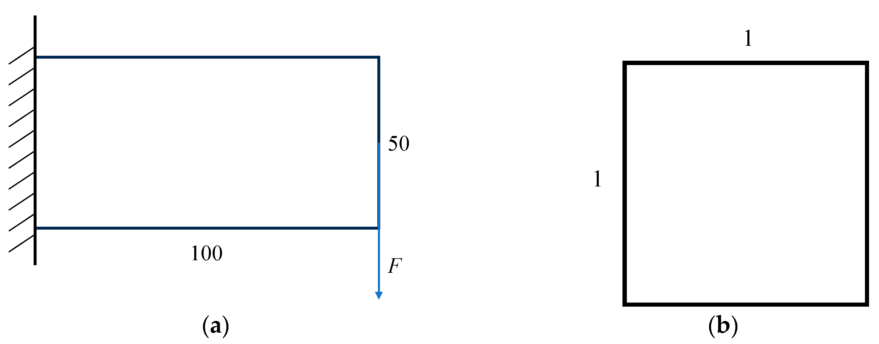
Figure 3.
Optimization convergence diagram of algorithms: (a) the objective function; (b) the volume constraint.
Figure 3.
Optimization convergence diagram of algorithms: (a) the objective function; (b) the volume constraint.
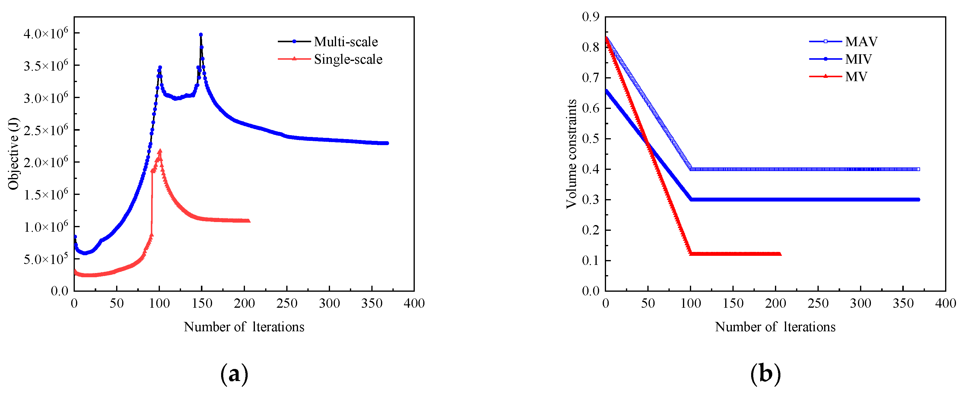
Figure 4.
Topology iteration for multiscale optimization: (a) macrostructural topology for multiscale optimization; (b) microstructural topology for multiscale optimization. n is number of iterations.
Figure 4.
Topology iteration for multiscale optimization: (a) macrostructural topology for multiscale optimization; (b) microstructural topology for multiscale optimization. n is number of iterations.

Figure 5.
Topology iteration for single-scale optimization. n is the number of iterations.
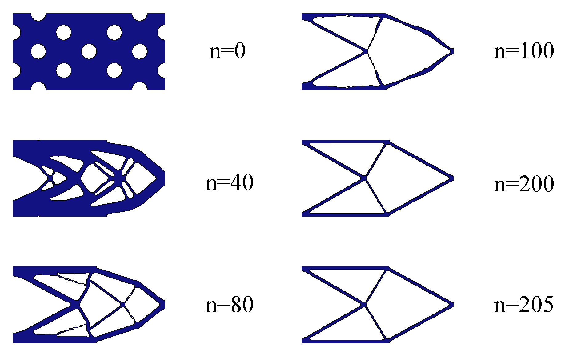
Figure 6.
Porous cantilever beam.
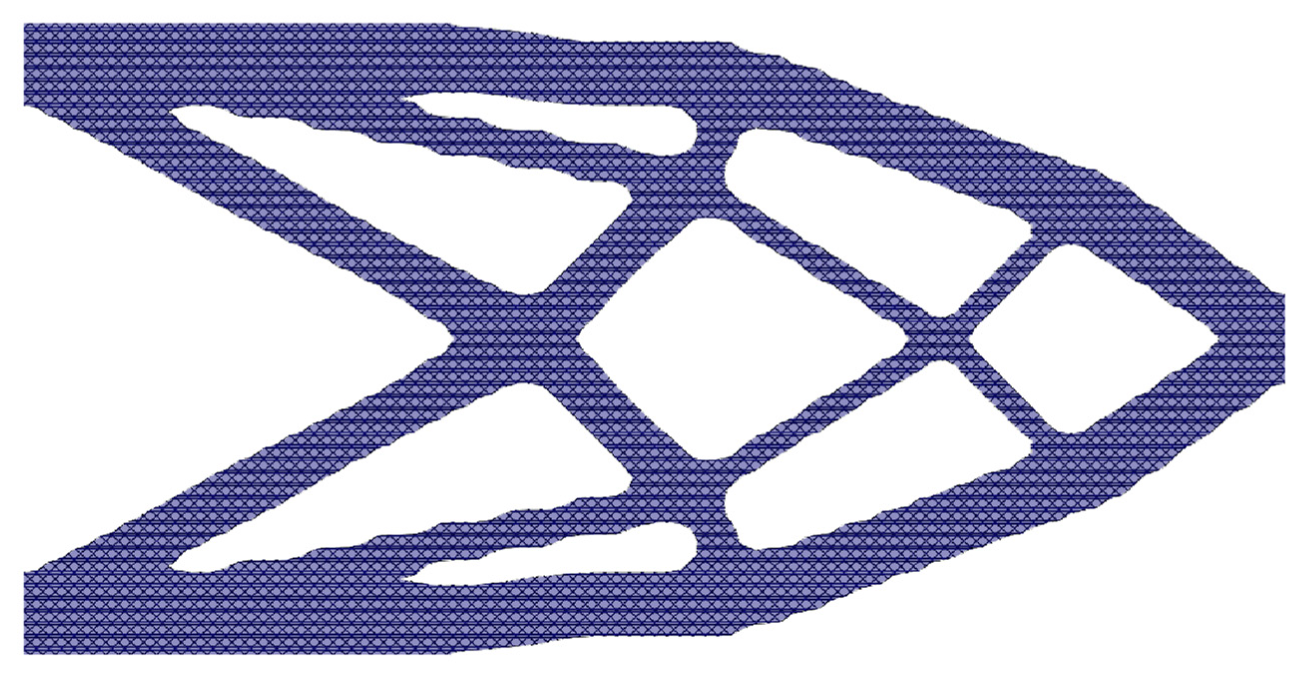
Figure 7.
The stress distribution of the structures obtained from: (a) multiscale optimization; (b) single-scale optimization.
Figure 7.
The stress distribution of the structures obtained from: (a) multiscale optimization; (b) single-scale optimization.
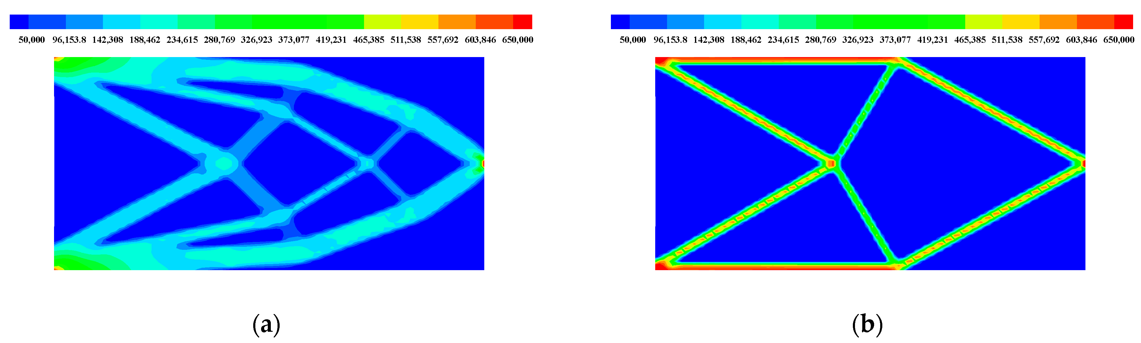
Figure 8.
Global Hawk UAV wing models: (a) geometry model of wing; (b) finite element model of wing.
Figure 8.
Global Hawk UAV wing models: (a) geometry model of wing; (b) finite element model of wing.
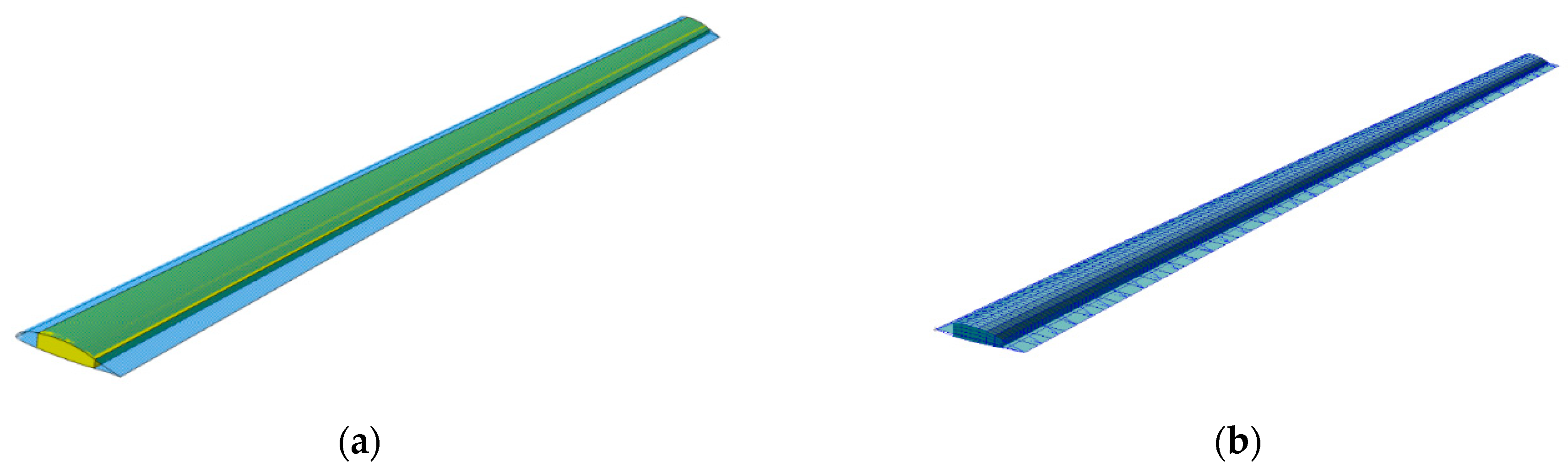
Figure 9.
Location of the initial spherical hole.
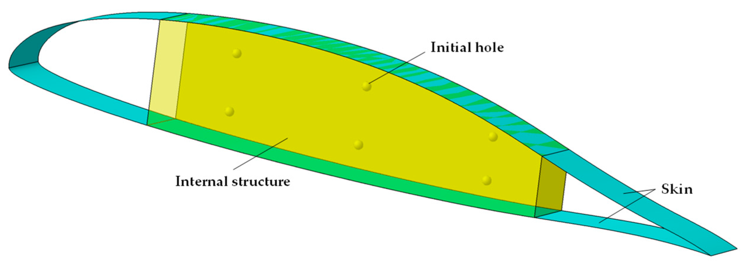
Figure 10.
Optimizing convergence diagram of algorithms: (a) the objective function; (b) the volume constraint.
Figure 10.
Optimizing convergence diagram of algorithms: (a) the objective function; (b) the volume constraint.
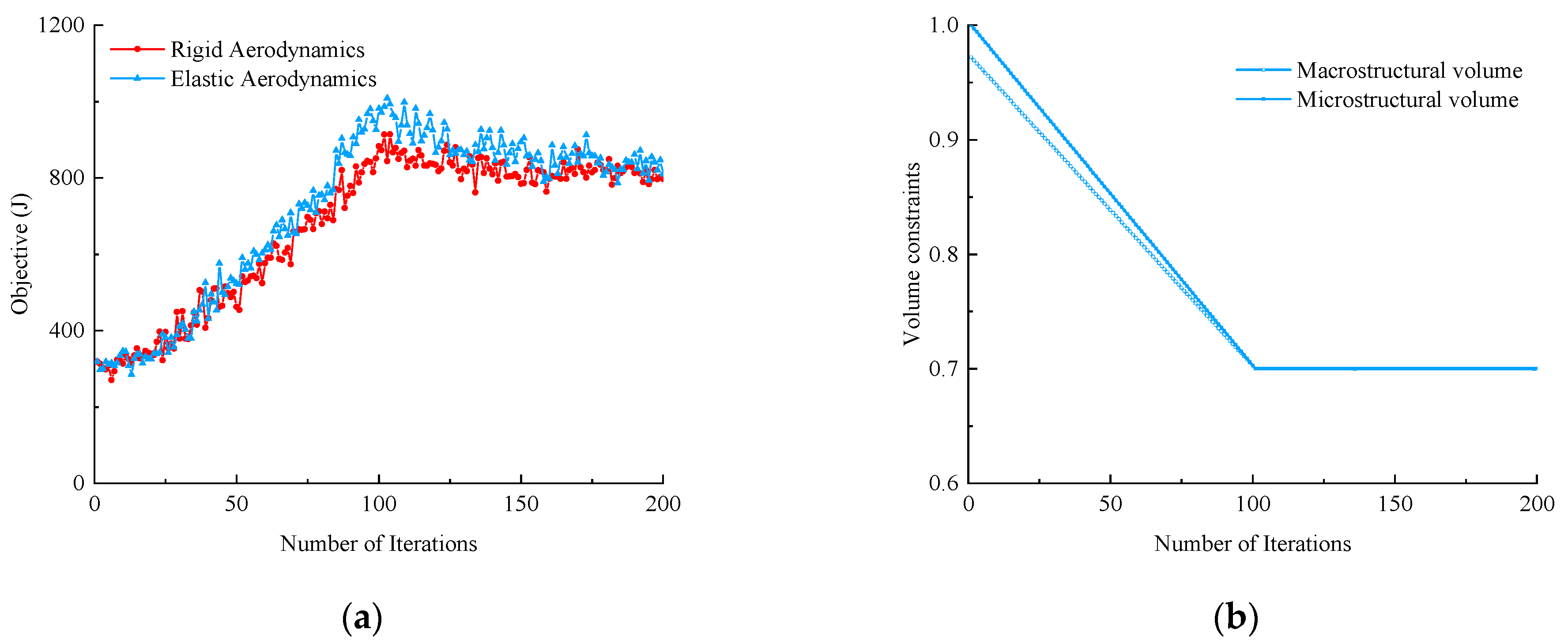
Figure 11.
Aerodynamic load distribution of the wing: (a) shear force distribution under aerodynamic load; (b) bending moment distribution under aerodynamic load.
Figure 11.
Aerodynamic load distribution of the wing: (a) shear force distribution under aerodynamic load; (b) bending moment distribution under aerodynamic load.
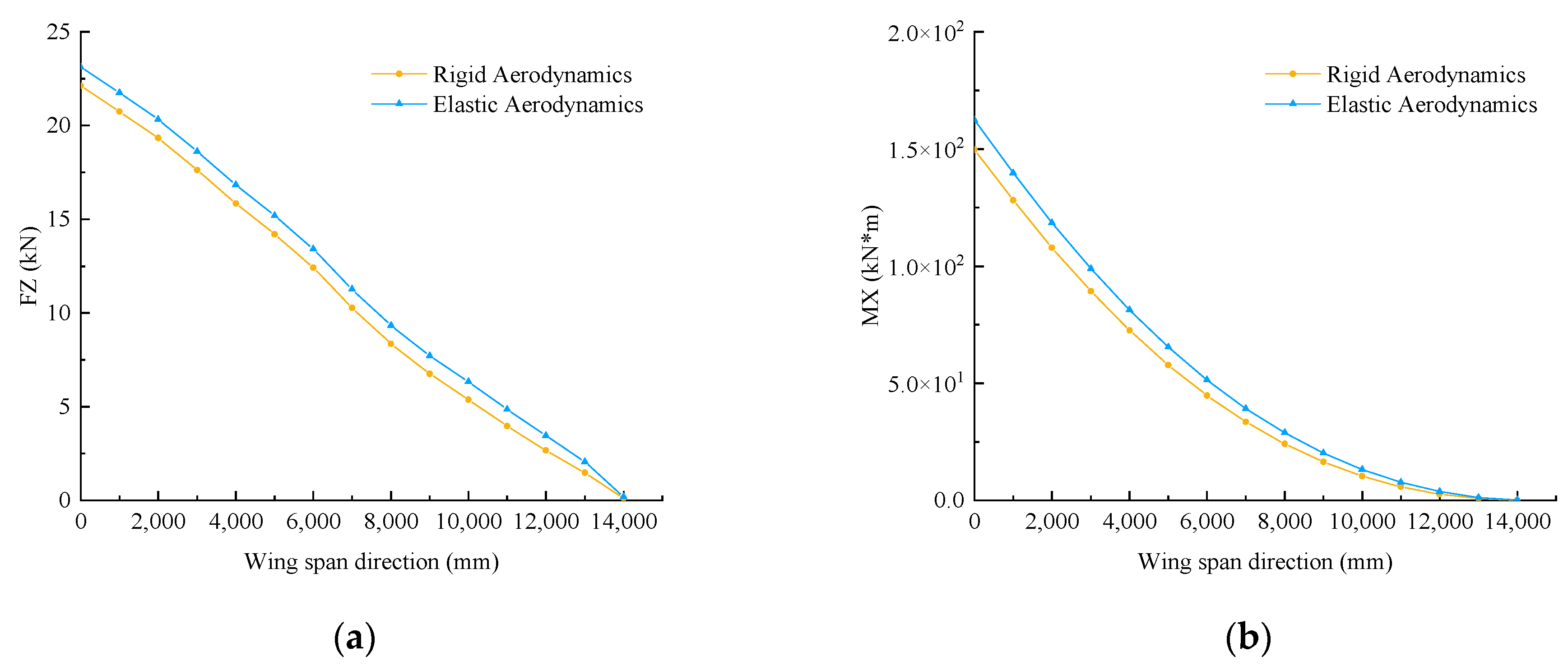
Figure 12.
Elastic component of aeroelastic forces.
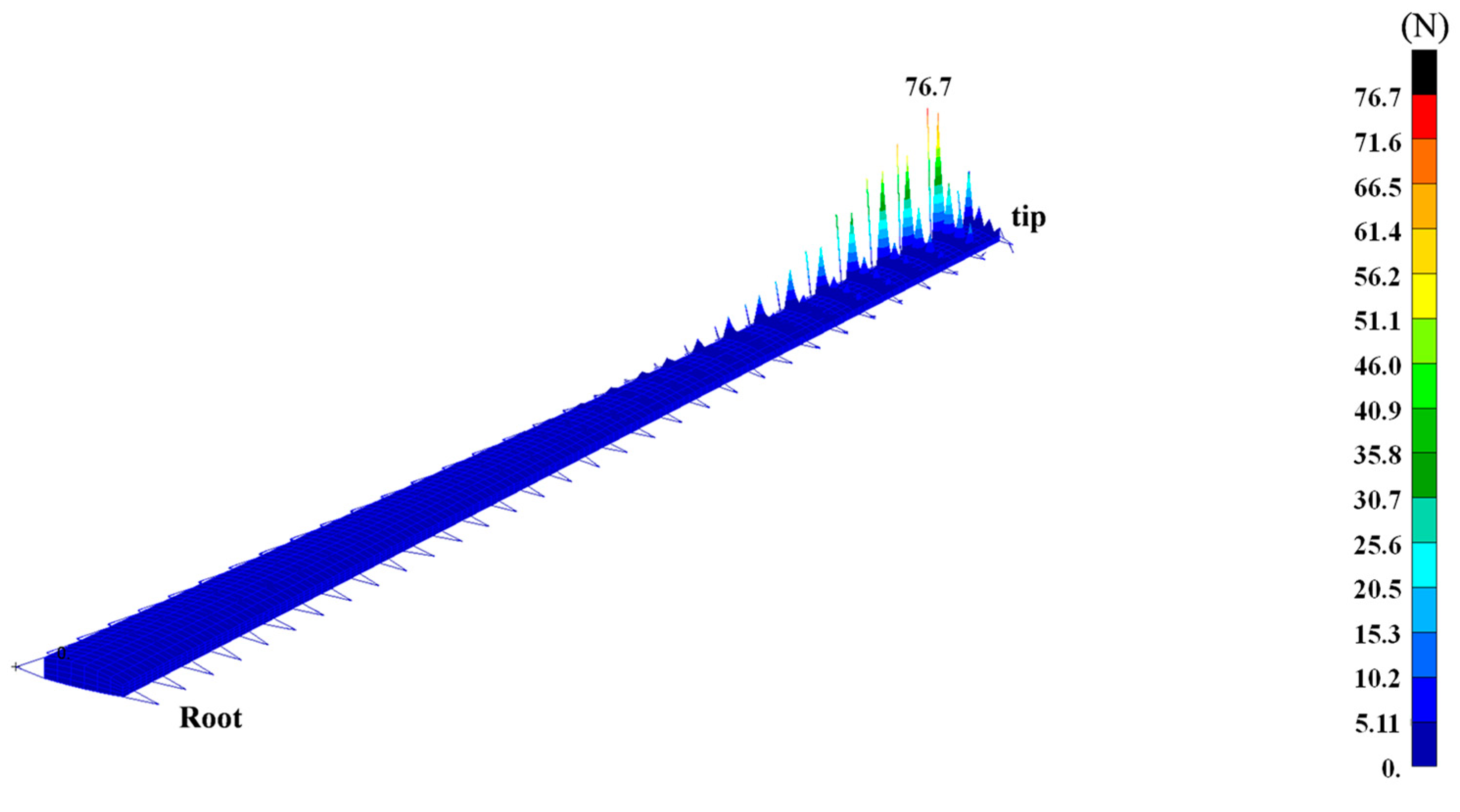
Figure 13.
Density of elements for the final macrostructure: (a) density of elements for the final macrostructure under rigid aerodynamic force; (b) density of elements for the final macrostructure under elastic aerodynamic force.
Figure 13.
Density of elements for the final macrostructure: (a) density of elements for the final macrostructure under rigid aerodynamic force; (b) density of elements for the final macrostructure under elastic aerodynamic force.
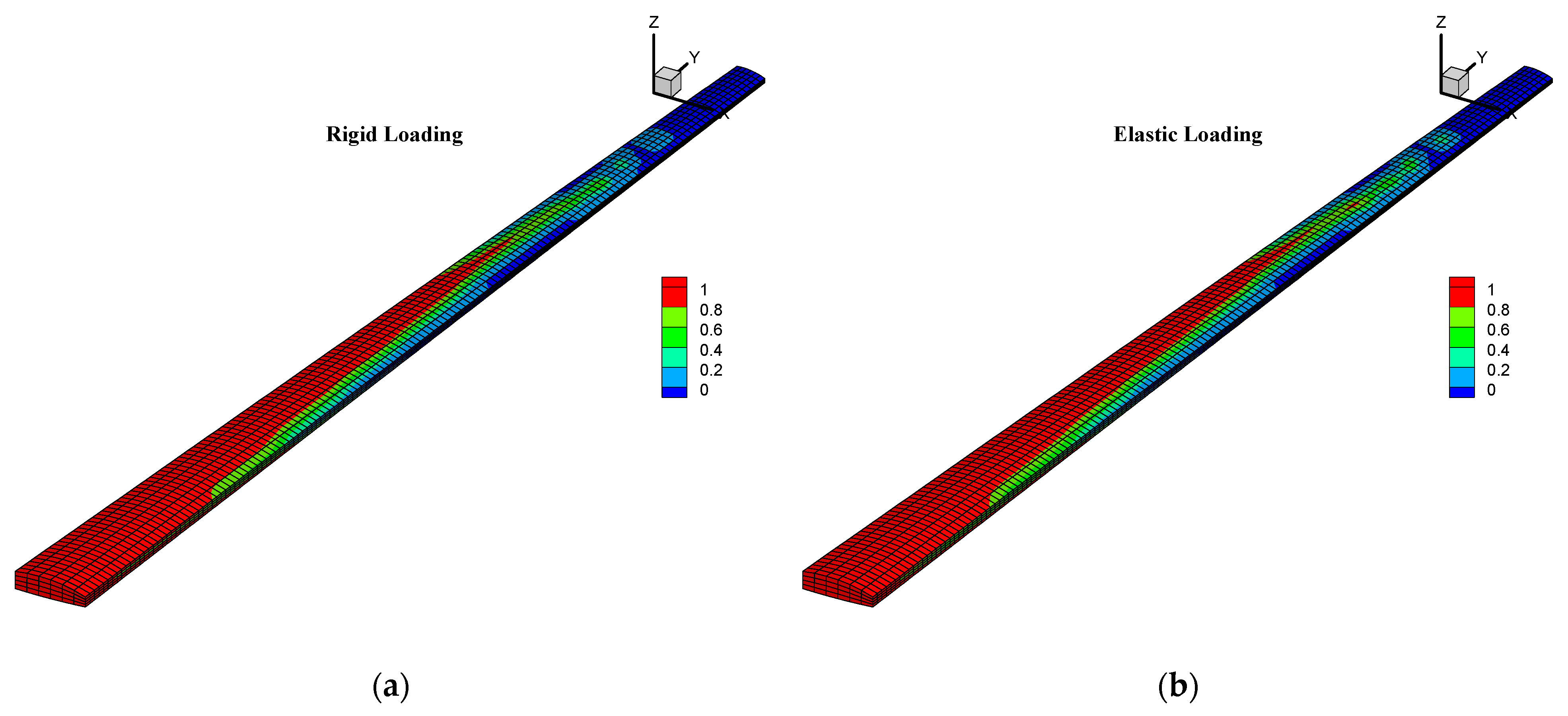
Figure 14.
Macrostructural topology under rigid loading: (a) macrostructural topology of optimization; (b) macrostructural topology of post-processing.
Figure 14.
Macrostructural topology under rigid loading: (a) macrostructural topology of optimization; (b) macrostructural topology of post-processing.
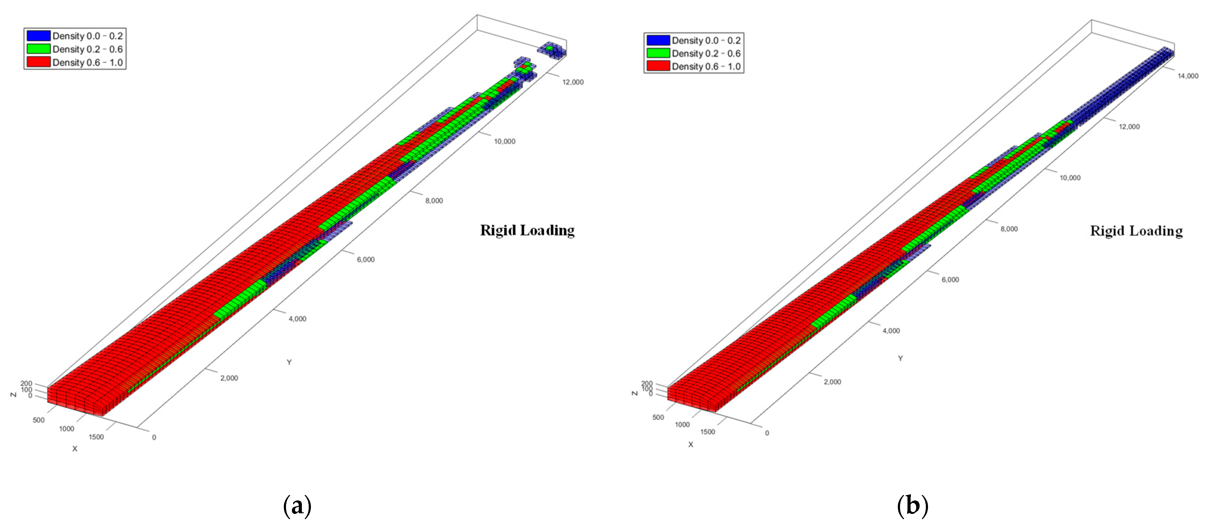
Figure 15.
The optimized microstructural structures under rigid loading.
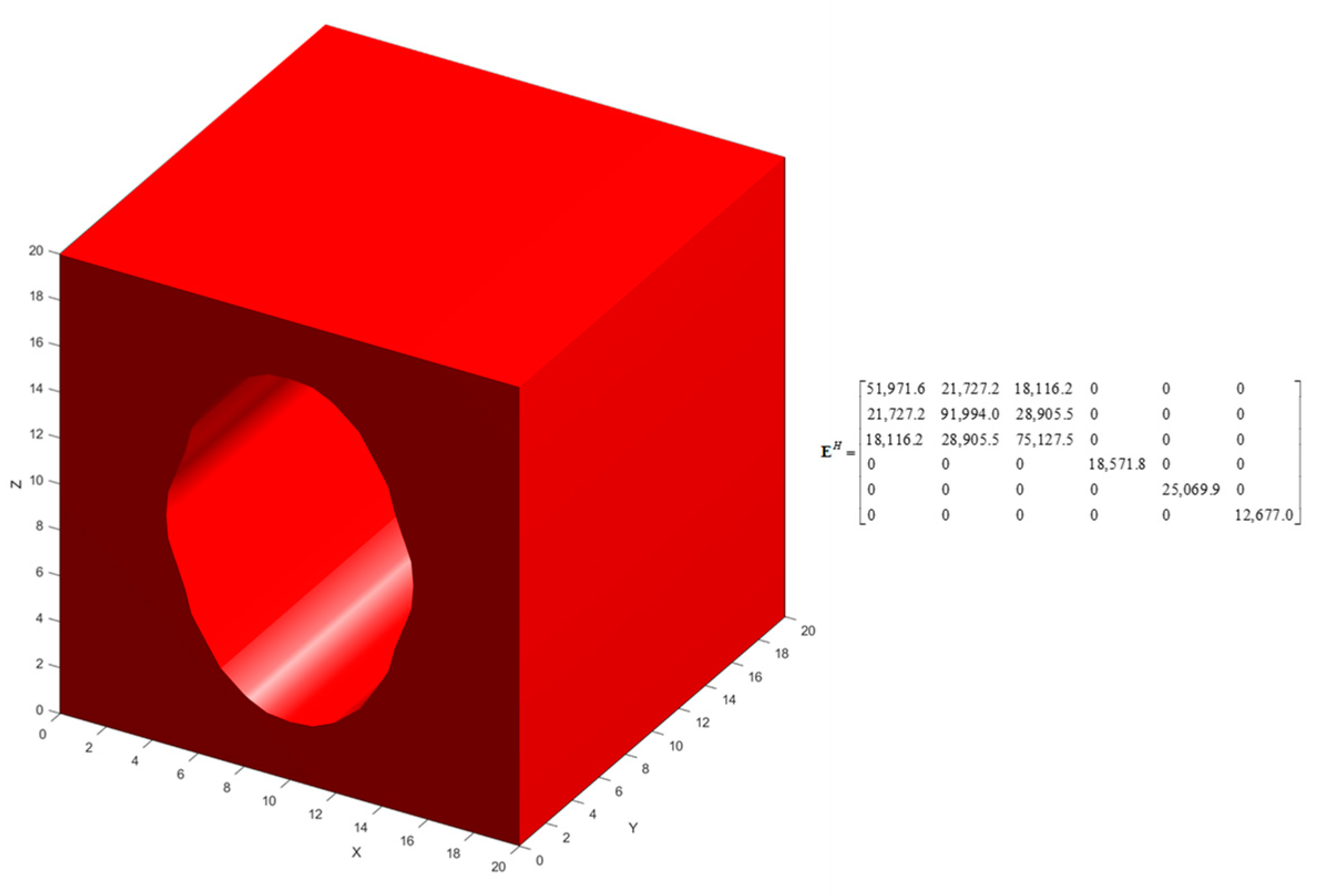
Figure 16.
The optimized macroscopic and microstructural structures: (a) macrostructural topology under elastic loading; (b) microstructural topology under elastic loading.
Figure 16.
The optimized macroscopic and microstructural structures: (a) macrostructural topology under elastic loading; (b) microstructural topology under elastic loading.
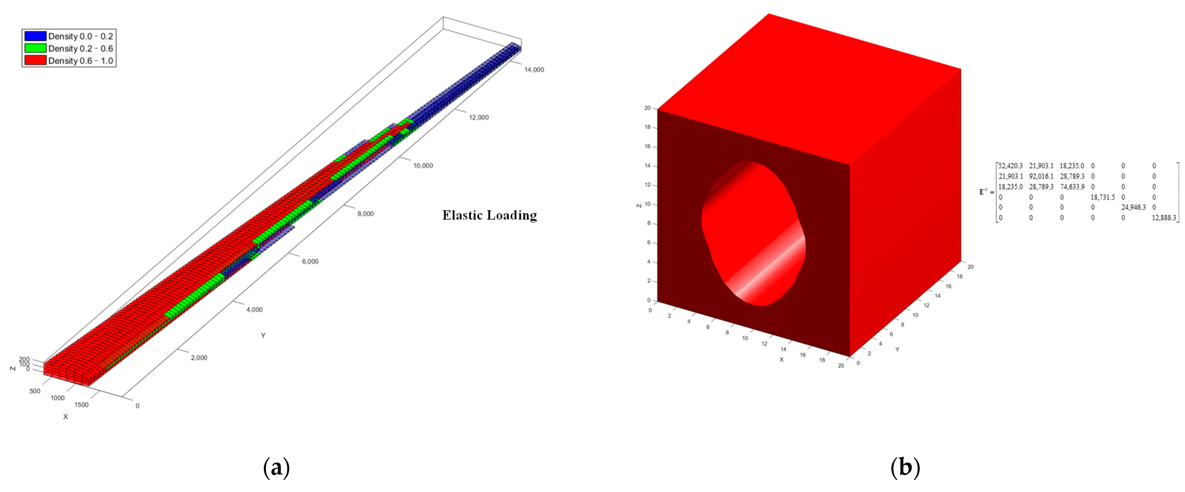
Figure 17.
Load distribution in the wing: (a) shear force distribution in the wing; (b) bending moment distribution in the wing.
Figure 17.
Load distribution in the wing: (a) shear force distribution in the wing; (b) bending moment distribution in the wing.
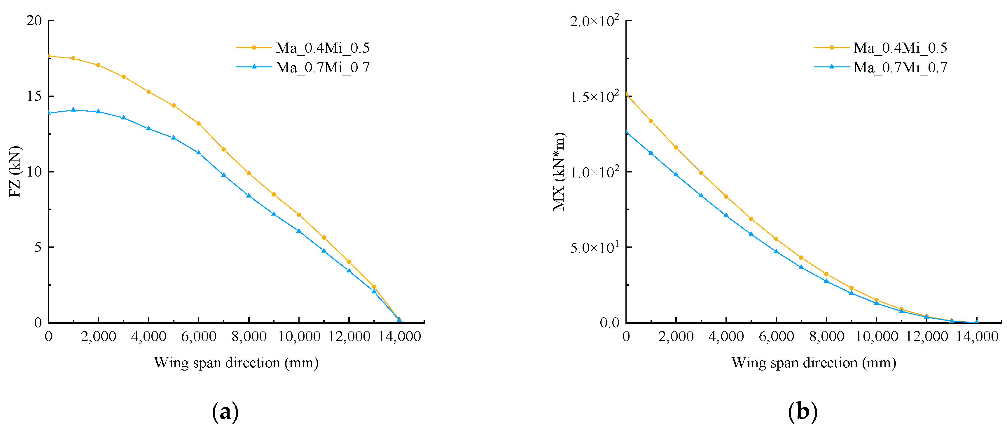
Figure 18.
Element density distribution in the wing: (a) density of elements in the final macrostructure; (b) ratio of percentage of element volume to total volume at different spanwise stations.
Figure 18.
Element density distribution in the wing: (a) density of elements in the final macrostructure; (b) ratio of percentage of element volume to total volume at different spanwise stations.
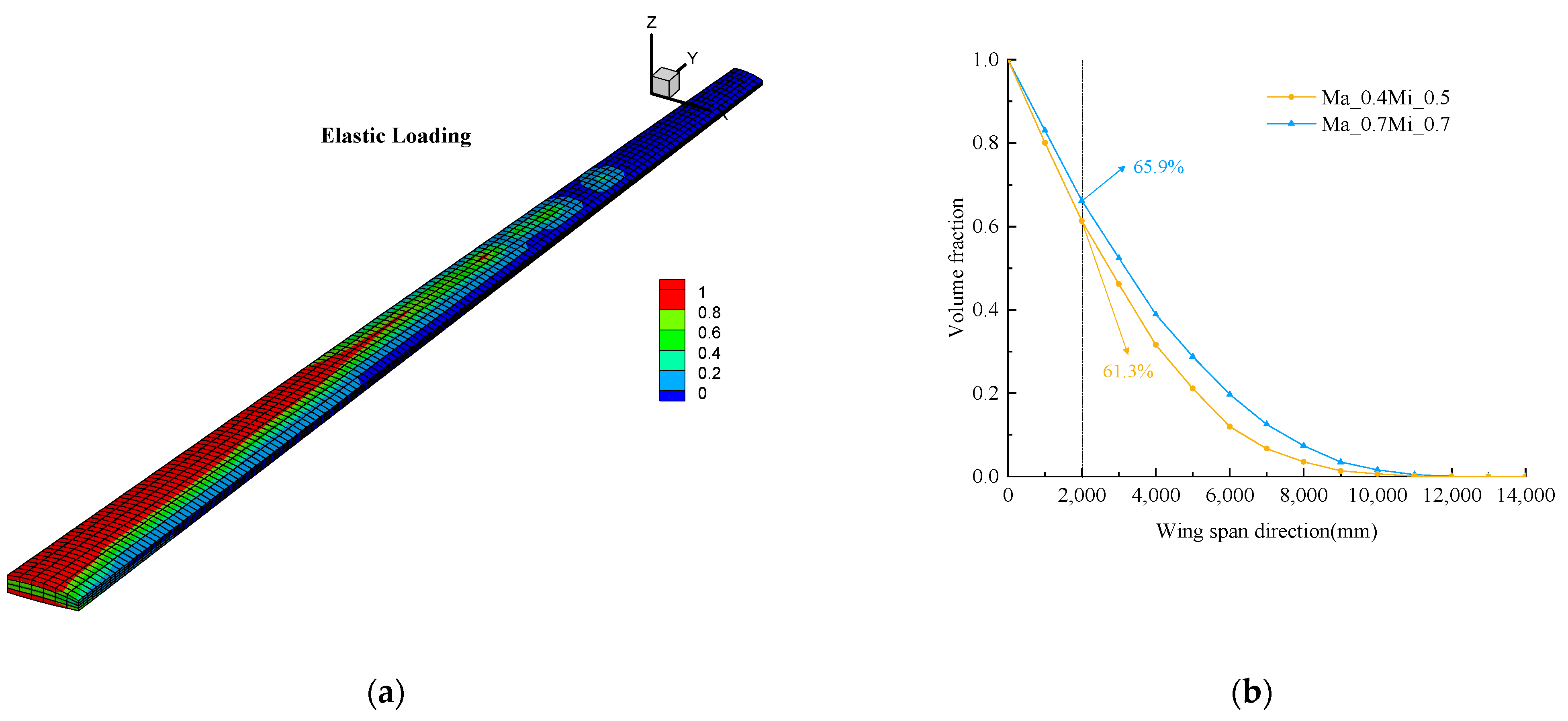
Figure 19.
The optimized macroscopic and microstructural structures: (a) macrostructural topology for Ma_0.4Mi_0.5; (b) microstructural topology for Ma_0.4Mi_0.5.
Figure 19.
The optimized macroscopic and microstructural structures: (a) macrostructural topology for Ma_0.4Mi_0.5; (b) microstructural topology for Ma_0.4Mi_0.5.

Table 1.
Optimization and post-processing results.
| Optimization Structure | Post-Processing Structure | |
|---|---|---|
| Compliance (J) | 7.62 × 10² | 8.47 × 10² |
| Mass ratio | 49% | 49% |
Table 2.
Optimization results.
| Ma_0.7Mi_0.7 (Rigid) | Ma_0.7Mi_0.7 (Elastic) | Ma_0.4Mi_0.5 (Elastic) | |
|---|---|---|---|
| Compliance (J) | 7.62 × 10² | 7.87 × 10² | 1.54 × 10³ |
| Mass ratio | 49% | 49% | 20% |
Disclaimer/Publisher’s Note: The statements, opinions and data contained in all publications are solely those of the individual author(s) and contributor(s) and not of MDPI and/or the editor(s). MDPI and/or the editor(s) disclaim responsibility for any injury to people or property resulting from any ideas, methods, instructions or products referred to in the content. |
© 2023 by the authors. Licensee MDPI, Basel, Switzerland. This article is an open access article distributed under the terms and conditions of the Creative Commons Attribution (CC BY) license (https://creativecommons.org/licenses/by/4.0/).
Share and Cite
MDPI and ACS Style
Li, K.; Yang, C.; Wang, X.; Wan, Z.; Li, C. Multiscale Aeroelastic Optimization Method for Wing Structure and Material. Aerospace 2023, 10, 866. https://doi.org/10.3390/aerospace10100866
AMA Style
Li K, Yang C, Wang X, Wan Z, Li C. Multiscale Aeroelastic Optimization Method for Wing Structure and Material. Aerospace. 2023; 10(10):866. https://doi.org/10.3390/aerospace10100866
Chicago/Turabian StyleLi, Keyu, Chao Yang, Xiaozhe Wang, Zhiqiang Wan, and Chang Li. 2023. "Multiscale Aeroelastic Optimization Method for Wing Structure and Material" Aerospace 10, no. 10: 866. https://doi.org/10.3390/aerospace10100866
Note that from the first issue of 2016, this journal uses article numbers instead of page numbers. See further details here.