A Proposed Exogenous Cause of the Global Temperature Hiatus

540 First Avenue West, Qualicum Beach, BC V9K 1J8, Canada
Climate 2019, 7(2), 31; https://doi.org/10.3390/cli7020031
Submission received: 10 January 2019
/
Accepted: 30 January 2019
/
Published: 3 February 2019
Abstract
:Since 1850, the rise in global mean surface temperatures (GMSTs) from increasing atmospheric concentrations of greenhouse gases (GHGs) has exhibited three ~30-year hiatus (surface cooling) episodes. The current hiatus is often thought to be generated by similar cooling episodes in Pacific or Atlantic ocean basins. However, GMSTs as well as reconstructed Atlantic and Pacific ocean basin surface temperatures show the presence of similar multidecadal components generated from a three-dimensional analysis of differential gravitational (tidal) forcing from the sun and moon. This paper hypothesizes that these episodes are all caused by external tidal forcing that generates alternating ~30-year zonal and meridional circulation regimes, which respectively increase and decrease GMSTs through tidal effects on sequestration (deep ocean heat storage) and energy redistribution. Hiatus episodes consequently coincide with meridional regimes. The current meridional regime affecting GMSTs is predicted to continue to the mid-2030s but have limited tendency to decrease GMSTs from sequestration because of continuing increases in radiative forcing from increasing atmospheric GHGs. The tidal formulation also generates bidecadal oscillations, which may generate shorter ~12-year hiatus periods in global and ocean basin temperatures. The formulation appears to assimilate findings from disciplines as disparate as geophysics and biology.
1. Introduction
1.1. Background
Variability in mean global surface temperatures (GMSTs) has generated varying and controversial claims about the attribution and interpretation of a ‘pause’ or ‘hiatus’ or ‘slowdown’ in temperatures that began around 1998 [1,2,3]. Fundamental questions include whether the phenomenon is real and meaningful. If it is real and statistically meaningful, then does it have a physical explanation? Is it forced or unforced? If forced, is it driven from within or by forces external to the climate system? Is it a singular or a repeated event? If repeated, then is it in principle predictable? Also and related to the hiatus, has global warming slowed or varied from modelled behaviour? If the hiatus is real and statistically meaningful and there is no widely accepted explanation for this suspension in temperature rise from anthropogenic global warming (AGW), then how can the scientific consensus concerning AGW be sustained? This paper offers an hypothesis involving exogenous forcing that may provide some clarity to this debate.
In the forefront of explanations for the hiatus is that it is an ocean surface phenomenon manifesting energy redistribution and heat uptake to the deeper ocean [2,3,4,5] but the mechanisms of heat redistribution vary for each basin [3,5]. On the basis of models of observed contemporaneous surface cooling patterns for particular ocean basins, energy redistribution during the episode has been suggested to originate from: the equatorial Pacific [6,7,8] and specifically the Interdecadal Pacific Oscillation (IPO) or Pacific Decadal Oscillation (PDO) [2,3,9]; the subpolar North Atlantic and specifically the North Atlantic Oscillation (NAO) [9]; and the subtropical Indian or Southern Oceans [5]. Yao et al. [10] proposed that the hiatus is a natural product of interplay between secular warming from GHGs and internal cooling by the cool phase of a quasi-60-year oscillation that is associated with the Atlantic Multidecadal Oscillation (AMO) and Pacific Decadal Oscillation (PDO). Kosaka and Xie [6] applied the Pacific Ocean-Global Atmosphere (POGA) experimental design to simulate the global warming hiatus, showing that global teleconnections were implicated in ocean circulation changes associated with the hiatus.
Physical simulations have met difficulty in reproducing the hiatus. Of 34 climate models in CMIP5 (the Coupled Model Intercomparison Project Phase 5), almost all were in accord with the established idea that subdecadal variability is associated with El Niño Southern-Oscillation (ENSO) activity but most models underestimated and gave different answers as to the cause of, the interdecadal variability that includes the hiatus [11]. The North Atlantic did not stand out as being particularly influential and models tended to attribute the cause to variability in the Pacific or Indian or Southern Oceans. Only ten of 262 model simulations with the Coupled Model Intercomparison Project Phase 5 (CMIP5) produced the early-2000s hiatus in global surface temperature rise from the decadal modulation associated with an IPO negative (cool) phase [12]. These results may indicate that an important factor is missing from the modelling.
1.2. Repeated Hiatus Periods from a 60-year Oscillation
The suggested post-1998 hiatus may be only the latest of several similar episodes. A cool episode in the 1940s was first suggested by Kincer [13]. Northern Hemisphere cool periods were documented from the late 1880s to 1910 and from about 1940 to 1970, with some limited support for the episodes from data over parts of the rest of the globe (in Wigley et al. [14] and the editors’ volume summary). It has been suggested that multi-year hiatus periods in global temperature can arise from the natural stochastic variability accompanying temperature increases through radiative forcing from atmospheric concentrations of greenhouse gases [15,16], a possibility acknowledged in the United Nations Intergovernmental Panel on Climate Change Fifth Assessment Report (IPCC AR5). That there have been more than one hiatus in GMSTs is often recognized (e.g. England et al. [17]), the sequence of hiatus periods being described as a GMST ‘staircase’ [7,9].
Some contrarians have suggested that global warming has stopped, by attributing the hiatus-punctuated rise in GMSTs to a combination of natural components that includes a repeated ~60-year oscillation. However, several studies (e.g. [18,19]) find a ~60-year oscillation in GMSTs after detrending the effects of increasing atmospheric concentrations of anthropogenic greenhouse gases.
Klyashtorin [20] associated a ~60-year oscillation found in the atmospheric circulation index (ACI) with alternating ~30-year zonal and meridional regime “epochs.” (A zonal flow occurs along a latitudinal or west-east direction and a meridional flow occurs along a longitudinal or north-south direction.) The ~60-year oscillation had a presence in the extent of ocean vertical advection (upwelling or downwelling) and of fish abundance; some species of fish respond to the cooler surface waters of meridional regimes while other species prefer the warmer surface waters of zonal regimes. Klyashtorin discussed the relationship between fluctuations in the earth’s rotation and the effects of changing velocities and latitudinal shifts of the winds during zonal and meridional atmospheric circulation regimes, this resulting in ~60-year oscillations in the length of day (LOD) and atmospheric angular momentum (AAM). Reviews [21,22] of temporal similarities between these multidecadal oscillations and indices of ocean basin variability have emphasized the distinction between zonal and meridional regimes each of about 30 years’ duration, with GMST cooling episodes occurring during meridional regimes.
In a 1400-year model of the AMO [23], the similarity of the simulated variability for a 70–120 year period to that for an observed 65 year period and the range of periods derived from paleodata, implied that “the AMO is a genuine quasi-periodic cycle of internal climate variability lasting many centuries and is related to variability in the oceanic thermohaline circulation.” Evidence for a ~70-year cycle has been found in Atlantic sea surface temperatures (SSTs) back to 1650 [24,25]. A ~60-year oscillation has been found in sea levels in every ocean basin during the 20th century but with different phases in different basins [26]. It has been found in a Labrador sea algae proxy for AMO SSTs since 1365 [27] and in LOD, AAM, ACI and fish catch as referenced previously.
From seven climate proxy records, including five Arctic ice-core records from Greenland and Canada and two tropical records (a lacustrine record from the Yucatan peninsula and a marine record from the Cariaco Basin), Knudsen et al. [28] found a 55- to 70-year component in 8000-year AMO proxy data and also detected an infrequent ~88-year component tentatively identified as the solar Gleissberg cycle. Separately, in two Holocene solar activity reconstructions they found a Gleissberg cycle but no ~60 year cycle and discounted the possibility of a solar source for AMO variability. An hypothesis presented in the next section will provide a possible alternative source for this ~88-year component. Kilbourne et al. [29] noted multi-century recurrences of a ~60-year oscillation, including a Puerto Rican δ18O coral proxy for Caribbean SSTs. The rising part of the δ18O proxy curve coincided with increasing upwelling of the planktonic foraminifer G. bulloides and with the timing of zonal regimes in Klyashtorin’s ACI.
These multiple sources of evidence for a repeated natural ~60-year oscillation suggest that this oscillation is a proximate cause of the hiatus periods. The larger question is of course to ask what the ultimate cause of this oscillation is. That there should be a similar oscillation with disparate geophysical, ocean, atmospheric and biological parameters seem at first mysterious. However, ocean upwelling is associated with variations in fish abundance [20] and with the ~60-year oscillation in the Puerto Rican coral proxy. Perhaps the major manifestation of ocean upwelling is to be found in the Atlantic Meridional Overturning Circulation (AMOC). In the introduction to their important review of the processes driving the AMOC, Kuhlbrodt et al. [30] state that the AMOC is a key player in the earth’s climate by virtue of its control on the distribution of water masses, heat transport and cycling of chemical species such as carbon dioxide and that "Ultimately, the influence of the Sun and Moon is responsible for oceanic and atmospheric circulations on Earth." These observations require an explanation for the ~60-year oscillation, the common zonal/meridional factor influencing geophysical and other parameters noted above and, in the present context, the hiatus. An hypothesis is described in the following section.
1.3. A Parameterization of Tidal Forces
Tidal forces derive from the differential gravitational force acting on a body that results from its varying distance from the gravitational source. The effects of tidal forcing on the oceans and on climate have followed a path benefiting from pioneering work by Doodson [31] and Cartwright and Taylor [32] among others. The tidal cycles derived reflect the intervals between similar orbital states of the sun or moon with respect to the earth. Doodson derived six fundamental astronomical frequencies ranging from a lunar day to nearly 21,000 years and developed further tidal frequencies f by adding or subtracting these frequencies or their harmonics, for example, f1 + 2f2 − f3. Doodson’s frequencies most relevant to explaining annual-to-multidecadal climate processes are those with fundamental periods 1, 8.847 and 18.613 years.
Keeling and Whorf [33,34] suggested that tidal forcing had climate effects through the periodic upwelling of water and resulting variation in sea surface temperatures (SSTs). Munk and Wunsch [35] investigated possible sources of ocean upwelling and found that the meridional overturning circulation may be mainly affected by the relatively small power of vertical mixing available. The winds and tides accounted for most of the abyssal mixing and the tidal power available from the sun and moon is 3.7 TW, more than half the power needed for vertical mixing in the ocean. A major focus of the present paper is to outline the sequence of steps by which tidally-generated oscillations may reproduce the surface temperatures that result in the hiatus phenomenon.
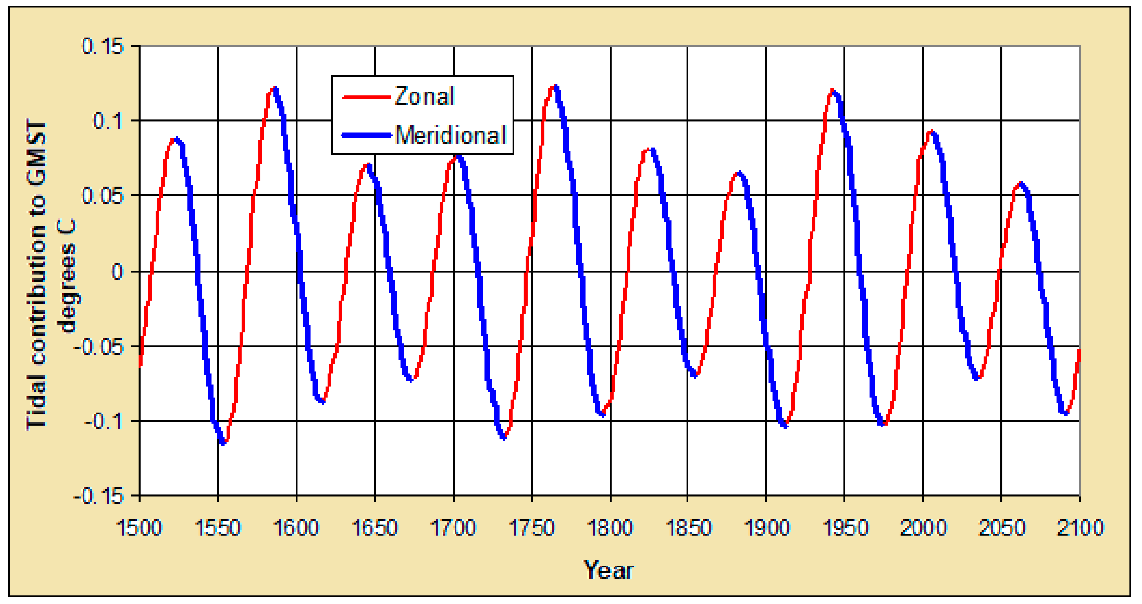
The tidal potential depends on the distances and directions of the sun and moon in relation to the earth. These distances and directions for a given time can now be calculated from astronomical polynomial algorithms, accurate over several centuries, from which we can obtain the separate mass/distance3 contributions from the sun and moon that capture the combined tidal forcing. In a 2002 paper by Treloar ([36], hereinafter T02), tidal forcing from the sun and moon was evaluated in three dimensions in order to include an accounting for the inclination of the (non-coplanar) orbital paths of the sun and moon as seen from earth. Tidal forces were then generated for orthogonal (essentially zonal and meridional) moments, with tidal oscillations derived in both orthogonal senses. Independently devising a “beating” procedure similar to that contemporaneously discussed by Keeling and Whorf [33], the initial high frequency tidal oscillations generated “beats” with tidal maxima at four lower-frequency components (T02), the components having major beats at intervals of 59.75, 86.81, 186.0 and (an irregular) 5.778 years.
Lorentzian envelopes for the three multidecadal components derived in T02 are shown in Figure 1, adapted from a 2017 paper by Treloar ([37], hereinafter T17). Tidal maxima for these beats coincided with a particular orbital orientation: when new moon coincided with unusually small perigee distances. The first (59.75-year) multidecadal component is zonal and the other two (with periods 86.81 and 186.0 years) are meridional in nature and analysis indicated relative amplitudes of 1700, 500 and 160 respectively. T17 described the three components (59.75-, 86.81- and 186-year) as ‘parents’ of the smaller ‘daughter’ components surrounding them, the latter having periods of 14.94, 21.70 and 18.60 years respectively (see Figure 1). The general maxima in these three sets can be given, in terms of near-contemporary dates or “reference dates,” as 2039.96 + nP1, 2039.96 + nP2 and 1918.20 + nP3 respectively, where n is a positive or negative integer and the P parameters refer to the respective periods. The tidal components were proposed to be related to climate oscillations as cosine forms cos[2π(t − 2039.96)/P] or cos[2π(t − 1918.20)/P], so that tidal and cosine extrema coincide.
It should be noted that the tidal parameterization in T02 and its zonal and meridional perspective, was developed without being aware of the zonal/meridional approach to the ACI by Klyashtorin [20]. Subsequently, his accumulation procedure was adopted in T17: the amplitude difference between multidecadal zonal and meridional forcing (Z–M) was accumulated over time to find the turning points between zonal and meridional regimes. In the tidal case, the accumulated difference was found between multidecadal zonal (59.75-year) and the major meridional (86.81-year) tidal component derived in T02. The result was a slightly irregular ~60-year oscillation produced by the modulation of the zonal by the meridional component and this oscillation was almost exactly in phase with the accumulated Z–M difference in Klyashtorin’s ACI. The timing of GMST hiatus periods was identified with the ~30-year regimes when the meridional component dominates the zonal as from the 1940s to 1970s; notable increases in GMSTs occur during ~30-year zonally-dominant regimes, as from the 1970s to around 2000. The δ18O coral multi-century proxy for Caribbean sea surface temperatures [29] also appeared to be in phase with the GMST tidal simulation in T17 Figure 2.
The three-dimensional analysis in T02 generated tidal periodicities infrequently mentioned in the literature, one exception being Wood [38]. The orthogonal formulation of the regime oscillations is unorthodox and may be unique, even though the analysis is underpinned by the standard physics inverse-cube relationship for tidal forces. T17 derived several further, mostly shorter-period, tidal oscillations from harmonics and frequency combinations of the T02 oscillations that were hypothesized to contribute to global mean surface temperatures.
T17 associated meridional tidal components with meridional ocean oscillations such as the AMO, IPO and PDO, while zonal tidal components were associated with zonal tropical oscillations such as the Oceanic Niño Index and Quasi-Biennial Oscillation. The proposition that exogenous tidal forcing generates both zonal and meridional oscillations means that we do not have to find a cause for each of the two sets of oscillations; tidal forcing parsimoniously simplifies the explanation. In the same vein, GMSTs were deconstructed in T17 to show that they could be simulated by combining the tidal ~60-year oscillation (and tidal frequency combinations and harmonics) with a curvilinear rise in global temperature, simulated by a power function, similar to the temperature response in published GHG emission scenarios. Apart from this combination of only two independent parameters (tidal forcing and the curvilinear rise), there appeared to be no evidence of contributions from 11- or 22-year solar cycles or from aerosols; there did, however, seem to be evidence for minor contributions from volcanic eruptions. This paper starts with the three multidecadal tidal components derived in T02 and the way they combine with the curvilinear rise from GHG-driven radiative forcing to create hiatus episodes in global temperatures. The paper then shows a link, through the tidal formulation, between global and ocean basin temperatures and further suggests that temperatures may also show evidence of shorter, decade-length hiatus periods.
2. Materials and Methods
This paper includes an update of the tidal hypothesis developed in T02 and T17 as it relates to GMST variability (particularly hiatus periods) and to surface temperature variability in the Pacific (reconstructions of the IPO and PDO) and Atlantic (reconstructions of the NAO) ocean basins.
The IPO is a pattern of ocean-atmosphere variability in trans-equatorial Pacific basin waters. The IPO exhibits decadal-scale warm (positive) and cool (negative) phases, referring to the temperature status of the eastern Pacific waters bordering the west coast of northern North America; during these phases, waters in the western north Pacific have the opposite temperature characteristics (cool and warm respectively). The PDO is a pattern of ocean-atmosphere variability, monitoring Pacific basin waters north of 20° N; it may be considered a northern cousin of the IPO. The PDO experiences similar decadal-scale warm (positive) and cool (negative) phases, with geographic patterns similar to the IPO. Eight reconstructions of these Pacific basin oscillations will be statistically compared with the three multidecadal tidal components and two of the reconstructions (one IPO, one PDO) will be examined in more detail.
The NAO is an irregular fluctuation measured by normalized surface level pressure difference between subtropical Azores (at the Azores High) and subpolar Iceland (at the Icelandic Low). The phases of the NAO are associated with significant modulations of zonal and meridional transport of heat and moisture. Low pressure over Iceland and high pressure over the Azores define positive phase of the NAO, which results in warm and wet winters in Europe and cold and dry winters in Northern Canada and Greenland. When the two pressures are weak, this represents the negative phase of the NAO and tends to produce cold temperatures in Europe and the US east coast. Five reconstructions of the NAO are statistically compared with the three multidecadal tidal components.
Testing the tidal hypothesis depends crucially on the timing of extrema (maxima or minima) in the tidal components, which depend on their various phases or, as characterized here, on their reference dates. The function used to test the presence of a component in a chosen global or basin oscillation is cos[2π(t − t0)/P], where P is the tidal component period in years, t is the decimal year at the oscillation datum and t0 is a reference date which is normally the time of a tidal maximum for the component in question. The temperature time series for an oscillation can then be regressed against tidal oscillation cosine functions to test the degree of correlation.
In the course of exploring the tidal formulation in the Results section, strong evidence will be presented to show that individual ‘parent’ (59.75-, 86.81 and 186.0-year) and respective ‘daughter’ (14.94-, 21.70- and 18.60-year) tidal components are present in the climate oscillations examined. This indicates that the tidal formulation generates ‘building blocks’ for understanding some of the dynamics of the climate system and the tidal components in Figure 1 are the threads that tie together all hiatus, ocean basin and global surface temperature results in this paper.
Results for the tidal hypothesis are developed in five sections:
(i) A simulation of the ~60-year GMST oscillation
A ~60-year oscillation in global temperatures is simulated by the modulation of the 59.75-year component by 86.81- and 186.0-year tidal components. The accumulated Z–M difference used in T17 to generate the ~60-year component in GMSTs is shown in Section 3.1 to be conveniently computed in an integrated form involving sine components and the formulation is expanded to include the 186.0-year component. The updated deconstruction of the ~60-year component in GMSTs, including components ranging down to subdecadal periodicities, is shown to be remarkably similar to a deconstruction by Schlesinger [39]. The bidecadal component in Schlesinger’s deconstruction is virtually identical to the bidecadal component generated in T17 by adding 21.70- and 14.94-year tidal components. The two deconstructions are consistent with the presence of three regularly spaced ~60-year GMST oscillations and accompanying hiatus periods in the historical temperature record.
(ii) On the timing and duration of the recent hiatus
The timing and duration of the recent GMST hiatus has been disputed, with differences of several years in various estimates of start and finish times; 40 different assessments of the starting and finishing years have been compiled [1] and the assessments compared to the tidal formulation. Since the ~60-year tidal component in global temperatures is simulated by the modulation of the 59.75-year component by 86.81- and 186.0-year tidal components, it necessarily implies the presence of the latter two tidal components in global or ocean temperatures. This proposition is examined in the following subsections.
(iii) An Interdecadal Pacific Oscillation (IPO) reconstruction from an Antarctic ice core
In contrast to the ~60-year oscillation component in GMSTs, this IPO reconstruction shows lower frequency oscillations, manifesting the presence of the 86.81- and 186.0-year tidal components.
(iv) A Pacific Decadal Oscillation (PDO) reconstruction
This reconstruction of the PDO incorporated principal components analysis to elicit three eigenmodes. Two of them are virtually identical to the 86.81- and 18.60-year tidal components in period and phase. The third component may be related to the tidal 21.70-year component but the correspondence may have been weakened by the inconsistent structure of the PDO over time.
(v) Multidecadal correlation patterns in ocean basin oscillations
Regression analysis on thirteen ocean basin oscillations for the presence of 59.75-, 86.81- and 186.0-year oscillations show a generally similar pattern in correlation signs of +, − and + respectively. The opposite signs for the first two, higher amplitude, components are consistent with the idea that zonal and meridional forces are essentially opposed or may not equally coexist and support the zonal-meridional (Z–M) difference adopted in Klyashtorin’s [20] original formulation for the atmospheric circulation index (ACI) and the similar tidal Z–M approach in T17 that led to simulating the ~60-year GMST oscillation.
3. Results
3.1. A Simulation of the ~60-year GMST Oscillation
The ratios of the 59.75- to 86.81- to 186.0-year amplitudes in Figure 1 are 1700:500:160 or more simply 3.4:1:0.32. Cosine relationships for the accumulated Z–M parameter over time t (in decimal years) were derived in T17 for the most significant 59.75-and 86.81-year components. Updating to include the 186.0-year component, a similar Z–M calculation involves accumulating the expression for the untreated, actual Z–M difference:
3.4cos[2π(t − 2047.96)/59.75] − cos[2π(t − 2047.96)/86.81] + 0.32cos[2π(t − 1926.20)/186.0]
The procedure in T17 for approximating the Z–M accumulation was needlessly complicated; the same result is obtained much more easily, since the accumulation over time is simply an integration. Accumulating this Z–M cosine expression and expanding to include the 186-year component, is equivalent to the simple sine expression:
3.4sin[2π(t − 2047.96)/59.75] − sin[2π(t − 2047.96)/86.81] + 0.32sin[2π(t − 1926.20)/186.0]
This expression provides a ~60-year oscillation amplitude for any decimal year t. The Z–M expression would lead one to expect negative signs for both meridional components and the positive sign for the 186.0 term will be explained below in Section 3.5.
The T02- and T17-defined dates of 2039.96 and 1918.20 are taken to apply to tidal responses at the ocean surface. In order to simulate the ~60-year oscillation in GMSTs in equations (1) and (2), the reference dates (2047.96 and 1926.20) adopted (T17) for the above three multidecadal components incorporate an empirical 8-year lag in relation to the T02-defined dates. The 8-year lag in the ~60-year oscillation was found to simulate GMST anomalies when accompanied by a curvilinear rise resembling responses to radiative forcing in GHG emission scenarios (T17). An important contribution to this rise is that the increase in atmospheric water vapor triggered by an initial warming due to rising carbon dioxide concentrations then acts to amplify the warming through the greenhouse properties of water vapor [40,41].
It was speculated in T17 that rising ocean temperatures during tropical zonal regimes acted to outgas GHGs at the ocean surface (perhaps promoted by tidal upwelling) and that increased global radiative forcing followed after an ~8-year migration of the GHGs to the upper atmosphere. This speculation was supported by:
- (a)
- a coupled model study by Huang et al. [42] that showed an increase in global AAM from an acceleration of zonal mean zonal wind in the tropical-subtropical troposphere;
- (b)
- AAM increases from the redistribution of mass when evaporation occurs over the oceans;
- (c)
- GMST rise is faster in zonal than in meridional regimes;
- (d)
- the appearance of similar 60-year cycles in the AAM, LOD, ACI and the multidecadal tidal oscillation, sometimes with small time lags between them, referenced above;
- (e)
- (f)
- striking similarities in the interannual variation in GMST anomalies, atmospheric carbon dioxide concentrations and proposed tidal oscillations (T17).
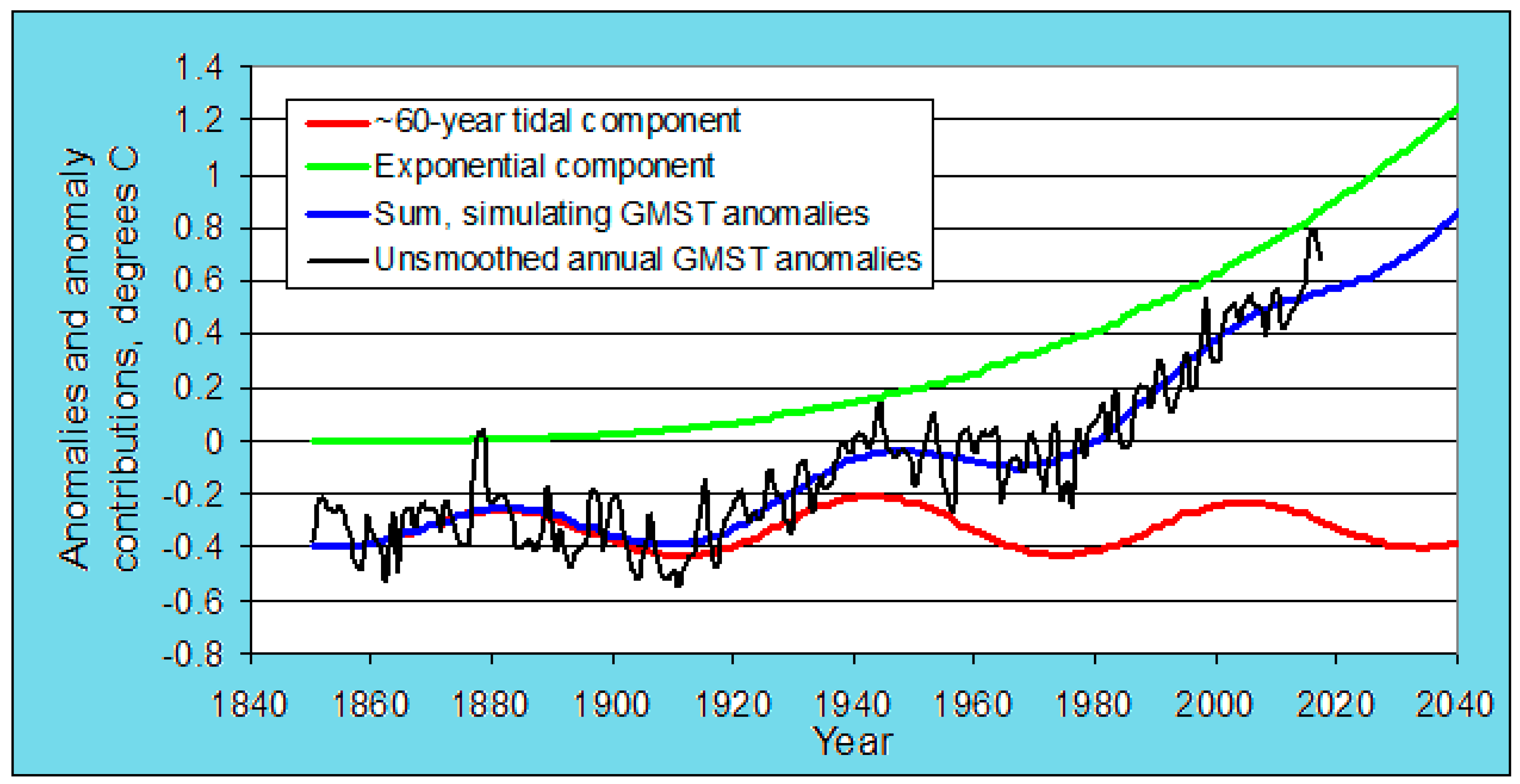
The ~60-year oscillation generated from the multidecadal tidal components can now be updated using the sine expression (2). With the iterative method in T17 including the annual GMST mean to 2017 from the Hadley Centre Climate Research Unit version 4 data set (HadCRUT4) [45], the tidal contribution to GMST anomalies is a multiple of 0.0265 times the sine expression (2) and the curvilinear rise in GMSTs ascribed to radiative forcing from atmospheric concentrations of GHGs is approximated by a power function relationship:
c (t − 1851.5)d where c = 3.65 × 10⁻⁷ and d = 2.87
The updated GMST simulation is shown in Figure 2.
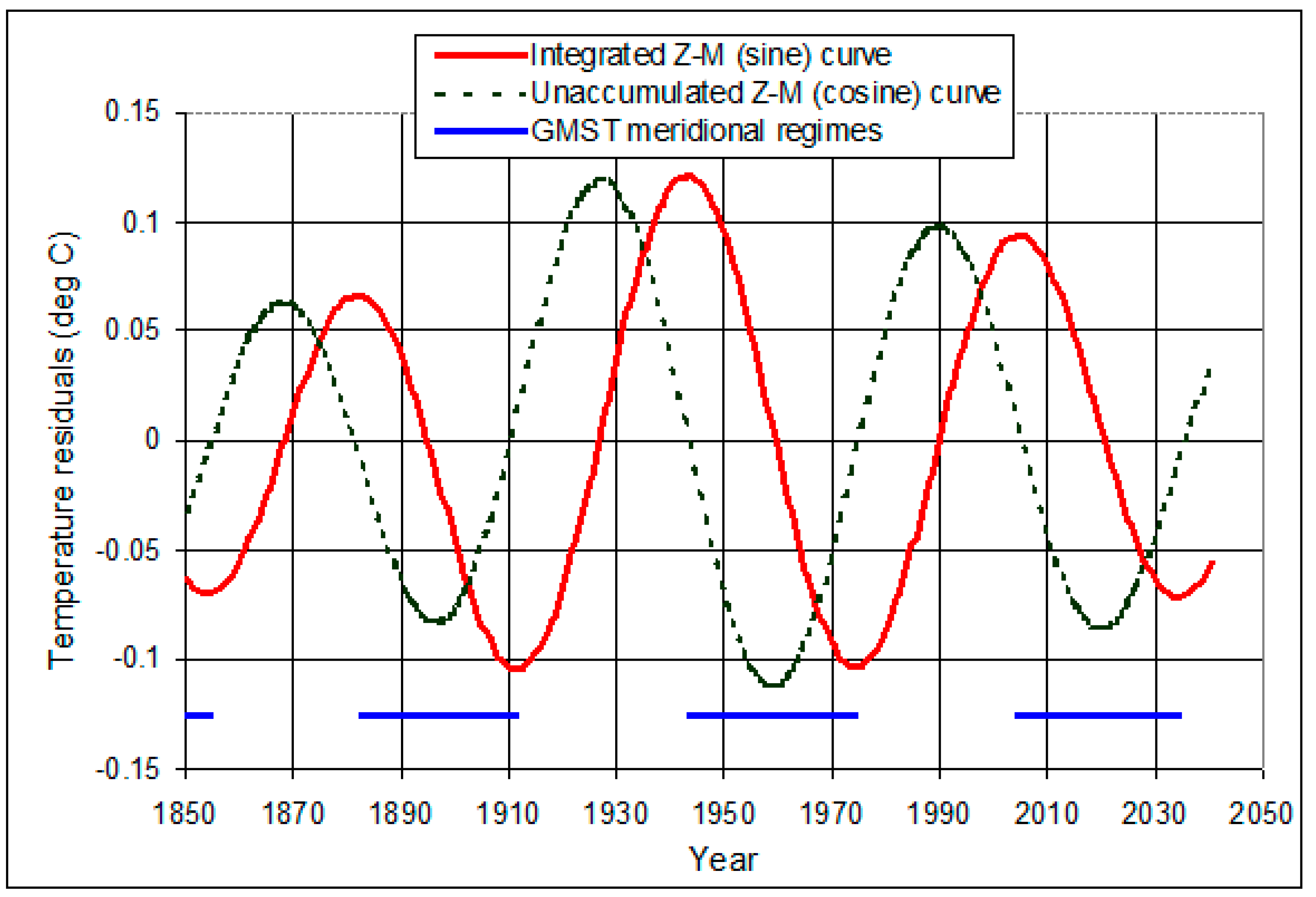
The ~60-year multidecadal tidal component is also shown in Figure 3 as the Z–M solid sine curve. Also shown is the corresponding (but here unaccumulated) cosine curve (dashed, from expression (1) above), which gives a measure of the rate of change in the tidal contribution. When Z > M, surface temperature is increasing, the dashed cosine curve is positive and the solid sine curve rises; when Z < M, surface temperature is falling, the dashed curve is negative and the solid curve falls. A rising solid sine curve segment indicates a zonal regime; a falling segment indicates a meridional regime. The curves are extrapolated to 2040.
The solid curve represents the multidecadal tidal modulation influencing the rise in the GMST response to increasing atmospheric GHG concentrations and the falling (meridional) segments of the curve since about 1850 are proposed to represent the timing of tidally-generated hiatus periods in GMSTs. The curve suggests a multidecadal-scale response to tidally-forced energy redistribution and transfer between the surface and the deep ocean. Figure 4 shows the expanded sine curve after the updating described. The parameterization shows turning points in years 1523, 1554, 1585, 1616, 1645, 1674, 1702, 1732, 1764, 1795, 1825, 1854, 1882, 1911, 1943, 1974, 2004, 2034, 2061 and 2090. The curve is very similar to AMO proxies (note Section 1.2 and the multi-century recurrences of a ~60-year oscillation in a Puerto Rican δ18O coral proxy for Caribbean SSTs and the AMO [29]). Inclusion of the 186.0-year component in the sine function makes only a small change in amplitudes and turning points from the T17 two-component ~60-year oscillation (RMS change ~0.01 °C). The alternating ~30 year rising (zonal) and falling (meridional) segments of Figure 4 are coloured red and blue respectively to emphasize a connection with warming and cooling contributions to GMSTs.
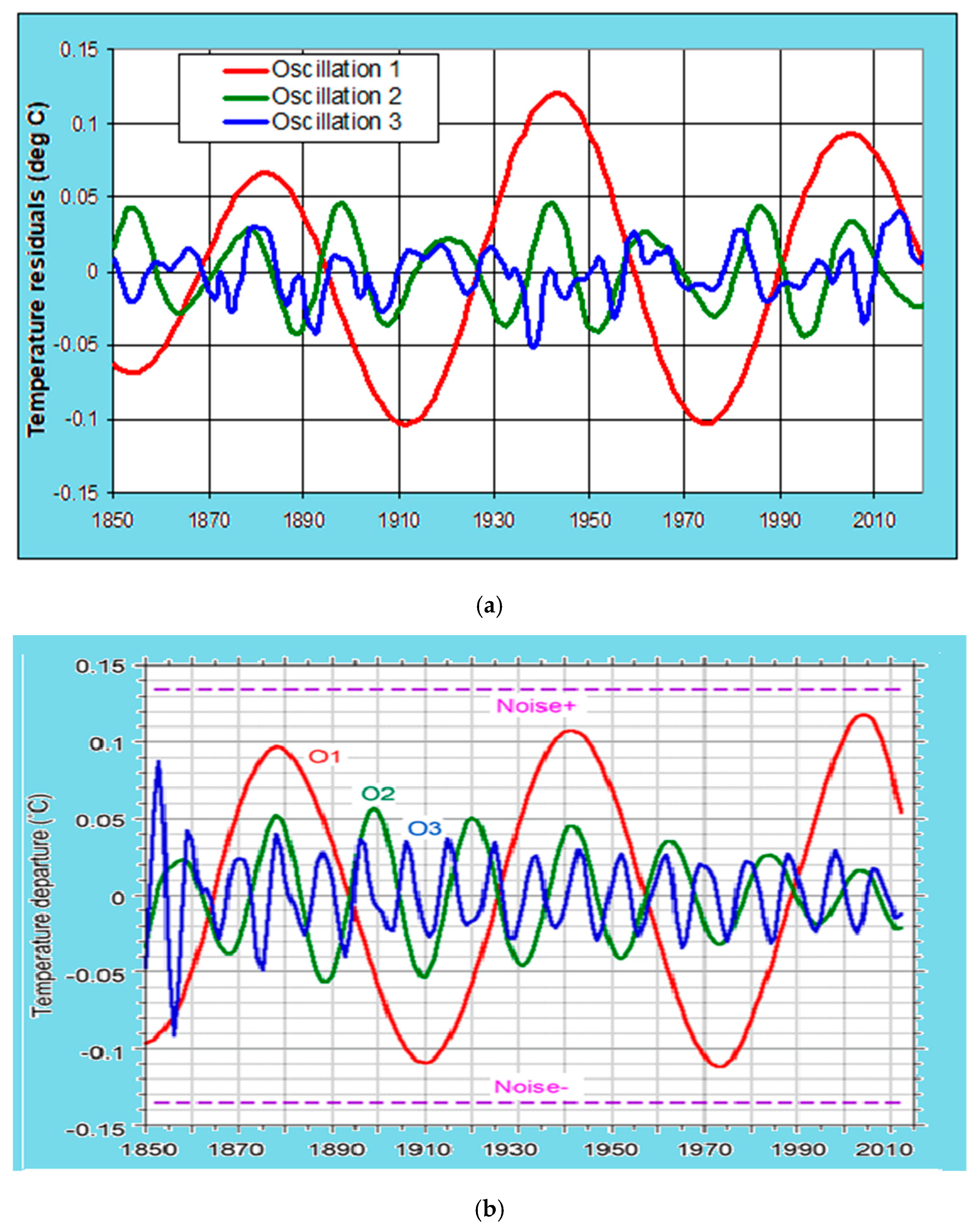
The multidecadal tidal ~60-year oscillation is shown as Oscillation 1 in Figure 5a. Higher-frequency harmonic and combination tidal components from T17 are also shown, to capture three timescales of variability (multidecadal, bidecadal and subdecadal) that contribute to the tidal simulation of GMSTs. Figure 5a was drawn to compare with a three-component sinusoidal deconstruction of GMSTs by Schlesinger ([39], Figure 5b). The two deconstructions are strikingly similar.
In Figure 5a: Oscillation 1 is a segment of the sine curves in Figure 3 and Figure 4. When the oscillation decreases, the result is a ~30-year meridional regime and a hiatus in GMSTs. The 2004 turning point represents the timing of the beginning of the recent hiatus from the tidal approach and the Figure by Schlesinger [39] seems to agrees with that timing.
Oscillation 2 is the sum of two bidecadal-to-decadal tidal components (the 14.94- and 21.70-year quarter-period ‘daughters’ of the 59.75- and 86.81-year ‘parent’ components) in T17 Figure 5; the two daughters can be seen in Figure 1 of the present paper.
Oscillation 3 is obtained by subtracting the above bidecadal-to-decadal variability from the six-component bidecadal-to-subdecadal variability in Figure 6 in the same source, in order to remove the duplicated bidecadal-to-decadal components. This generates the irregular subdecadal temperature response in Oscillation 3 because the bidecadal-to-subdecadal component amplitudes change between zonal and meridional regimes.
3.2. On the Timing and Duration of the Recent Hiatus
Lewandowsky et al. [1] compiled 40 different assessments of the beginning and end of the recent hiatus. Some of the assessed start and finish years were slightly ambiguous but the years centred on a few particular ones. Starting years for the hiatus ranged from 1993 to 2003, with the ‘most favoured’ years being 1998 and 2000 (representing a total of about half of the assessed starting years), followed by 2001; the other years had a much smaller representation. End years for the recent hiatus in the compilation ranged from 2008 to 2013, with 15 of 40 of those years assessed to be 2012, followed by 9 for 2013, then decreasing numbers for 2010, 2009 and 2008. The median beginning and end years were 2000 and 2012, giving a 12-year duration. However, the tidal hypothesis indicates (Section 3.1) that the present meridional regime began in 2004 and will continue until 2034, consistent with the ~30-year meridional timescale.
It seems there is no currently agreed, expected or theoretical duration for a hiatus. The ~30-year durations for three hiatus episodes are consistent in the Schlesinger and Treloar deconstructions, each episode representing the cooling half of a ~60-year oscillation. If a generally recognized hiatus is found to have a 12-year duration and this is taken as the cooling half of a higher-frequency oscillation, then that oscillation would have a period around 24 years. Interestingly, the bidecadal component (Oscillation 2) in Figure 5a has a mean period of 21.7 years, since it is dominated by the 21.70-year meridional ‘daughter.’ The minimum and maximum in that curve corresponding to the medians in the Lewandowsky et al. compilation occur during 2005 and 2019. A conceivable explanation for the discrepancy between the two sets of results may lie in the difficulty of characterizing a decadal-scale hiatus in GMSTs in the presence of an accompanying ~60-year oscillation and a rising background from radiative forcing due to atmospheric GHGs. However, the possibility exists that we may encounter a combination of both ~30- and ~11-year hiatus periods (the latter from bidecadal oscillations) in global and ocean basin temperatures.
The possibility that El Niño events influence estimates of the timing of hiatus episodes is examined in the Discussion section. However, tidal forcing is exogenous and essentially deterministic and should not generate the hiatus as a stochastic process. Consequently, it should provide no uncertainty about the hiatus start and finish if identified with times when the ~60-year curve enters and leaves its meridional phase; the tidal turning points are consequently defined.
An interesting question is whether cooling from tidally-forced ocean energy redistribution and heat uptake during the regime can now overcome the curvilinear temperature increase by radiative forcing from increasing atmospheric concentrations of GHGs. Updating the T17 iteration procedure as mentioned in the last section, the power function expression representing the curvilinear response to the radiative forcing from increasing atmospheric GHG concentrations is amended to 3.65 × 10⁻⁷ × (t − 1851.5)2.87, where t is the decimal year at a post-1851.5 time. The annual increase in the power function expression at time t is the gradient, equal to about 1.05 × 10⁻⁶ × (t − 1851.5)1.87 and the decadal change is ten times that. Mid-meridional regime times in Figure 3 and Figure 5a are 1896.5, 1958.5 and 2019.0, which therefore imply respective decadal temperature increases from the curvilinear rise to be 0.013, 0.065 and 0.151 degrees C. In contrast, the mid-meridional regime decadal temperature decreases in the solid curve in Figure 3 are in the range 0.08 to 0.1 degrees C. It is therefore clear that, while the first two meridional regimes do produce a ~30-year cooling episode on this parameterization, the third and subsequent meridional regimes would not (assuming GHG concentrations continue to increase); the rise in radiative forcing from atmospheric GHG increases will override that cooling. The cooling segments in Oscillation 2 of Figure 5a, representing a near-bidecadal contribution to GMSTs (from 14.94- and 21.70-year tidal components), are also of a magnitude that would be overridden in future by the background curvilinear increase from GHG atmospheric concentrations.
GMSTs since 1850 have been simulated as the summation of (a) a power function expression for the radiative forcing from atmospheric GHGs and (b) a three-fold recurrence of the ~60-year oscillation derived from a parameterization of tidal forcing (the latter being essentially deterministic). This is inconsistent with a view that the hiatus is generated stochastically. However, stochastic natural fluctuations in sea surface temperatures may be important locally.
It has been noted (Section 1.1) that the recent GMST hiatus has been linked to contemporaneous cool episodes in ocean basin oscillations such as the IPO, PDO and NAO. If the tidal approach to GMSTs invokes the three multidecadal (59.75-, 86.81- and 186.0-year) components to explain the hiatus, then the same three components should also be found in ocean basin oscillations. Each of these is expected to include the 8-year lag associated with hypothesized zonal regime evaporation and subsequent atmospheric rise of GHGs (Section 3.1). This is explored in the next sections.
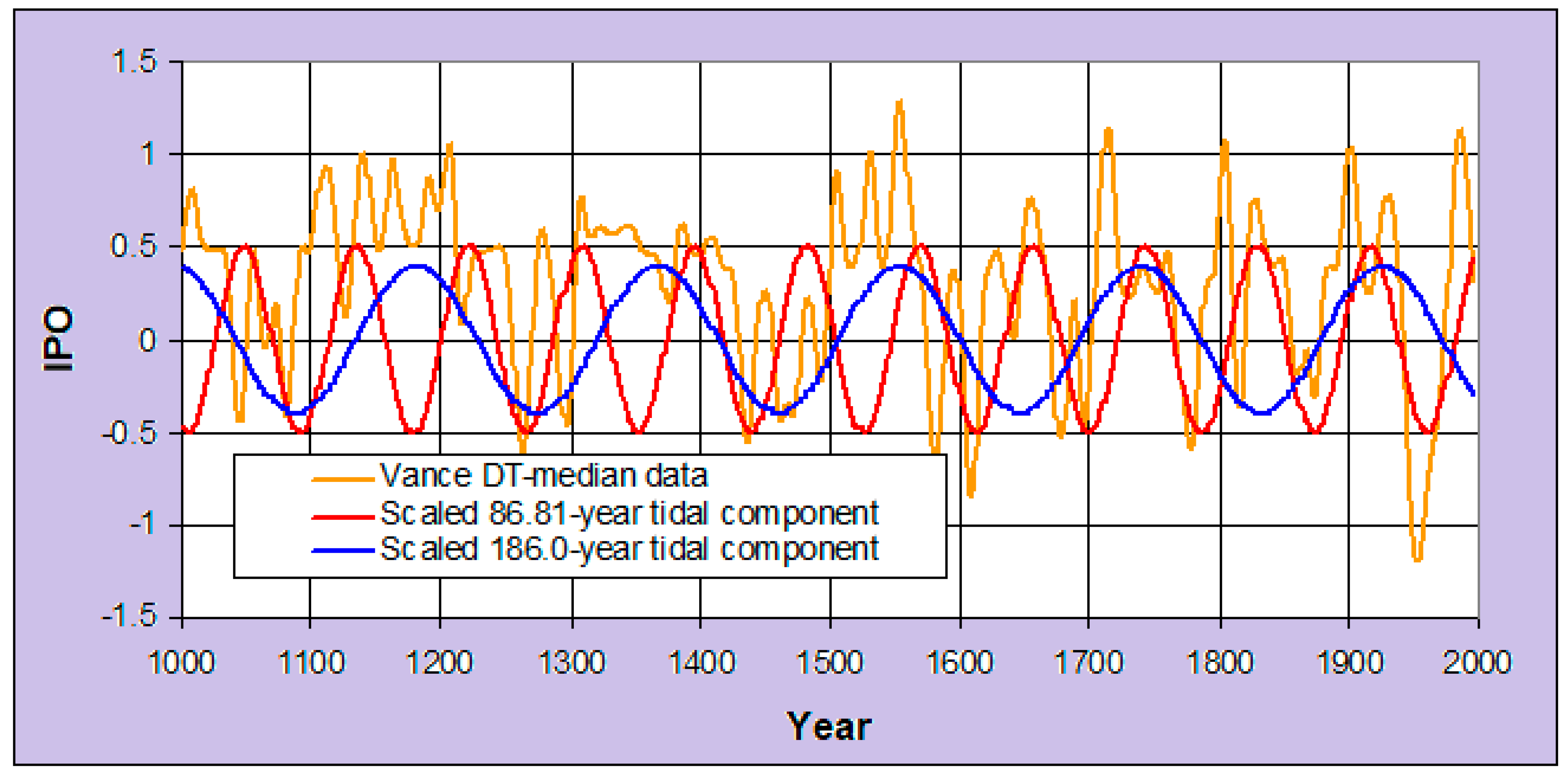
3.3. An Interdecadal Pacific Oscillation (IPO) Reconstruction from an Antarctic Ice Core
Using piece-wise linear fit (PLF) and decision tree (DT) reconstruction methods, Vance et al. [46] generated a near-1000-year IPO reconstruction from sea salt content in an ice core from the Law Dome site in the Antarctic. With the timing of tidal maxima (2047.96 + 59.75n for the 59.75-year component, 2047.96 + 86.81n for the 86.81-year component and 1926.20 + 186.0n for the 186.0-year component, where n is a negative or positive integer), regression shows a significant zonal 59.75-year component but much more significant meridional 86.81- and 186.0-year components, the latter with probability p values of 5.4 × 10⁻²² and 10.9 × 10⁻²⁶ and with t statistics of −9.9 and +10.9 respectively. The DT-median reconstruction is shown in Figure 6, with vertically scaled contributions from the meridional components. Consistent with the Z–M formulation and equation (1), the sign of the cosine function for the meridional 86.81-year component is negative and that for the meridional 186.0-year cosine function is positive.
Figure 6 shows no notable presence of ~60-year oscillations. Rather, it suggests longer duration changes in temperature, produced by the mix of meridional 86.81- and 186.0-year oscillations. The curve suggests a transition around 1600 between the relative contributions of the two components. If real, the transition may be related to the time of an abrupt 10 ppm decrease in greenhouse gas content as recorded [47] in an ice core from (again) Law Dome. The high southern latitude (−66.8° S) of the Law Dome site may help to explain the dominance of meridional contributions. The roughly equal vertical scaling for the two components in Figure 6 varies from the previously calculated relative amplitudes of 1:0.32 and the reason may be a region- or latitude-dependent one.
The two meridional components are anti-correlated in relation to their tidal maxima (as evidenced by the signs of the t statistics) and this will be observed for results in ocean basins in following subsections. The reason for this anti-correlation is unclear but the pattern in the signs for cosine functions is explored in a broader context in Table 1 below.
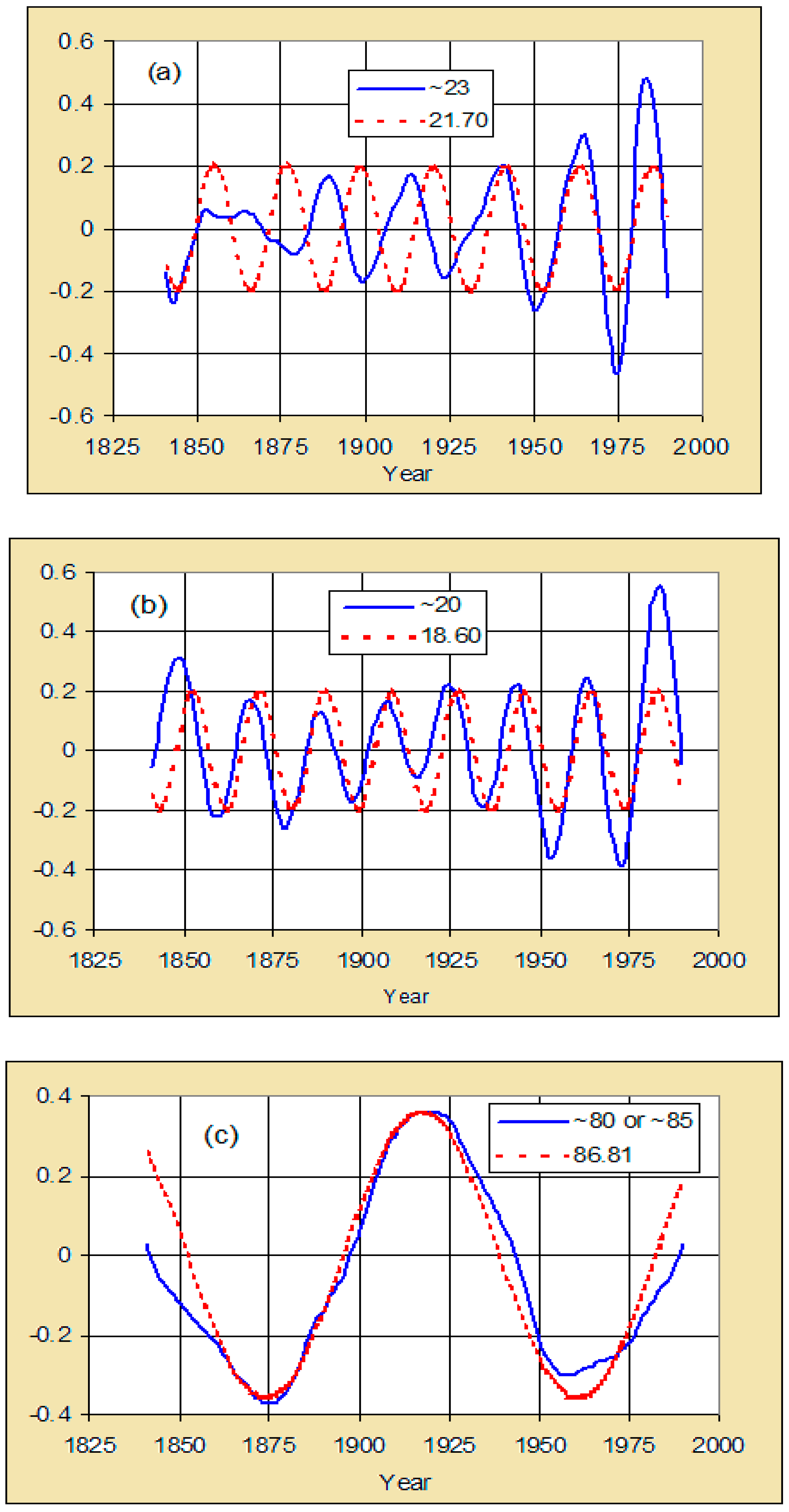
3.4. A Pacific Decadal Oscillation (PDO) Reconstruction
Gedalof et al. [48] used principal components analysis to find common modes of variance in five climate reconstructions around the North Pacific Basin that link to extratropical interdecadal variability. Using singular spectrum analysis, three eigenvectors were extracted, producing PDO components with periods of around 23, 20 and 80–85 years. These components are shown in Figure 7a–c, overlapped with vertically scaled tidal components with periods 21.70, 18.60 and 86.81 years with their respective defined phases. The respective expressions for the components are: −0.2 cos[2π(t − 2039.96)/21.70], −0.2 cos[2π(t − 1918.20)/18.60] and −0.36 cos[2π(t − 2047.96)/86.81]. The latter component incorporates the 8-year lag derived for the three multidecadal components in T17, to account for the time for GHGs to migrate to the upper atmosphere. The first two, like all other components derived in T02 and T17, are assumed to act at the ocean surface and assigned a zero lag time. See Section 3.1 above.
The scaling in these Figures incorporates sign-reversal for all three tidal cosine components. This implies that maxima in tidal forcing (times when close perigee tends to occur at new moon) correspond to lower temperatures and perhaps greatest upwelling. The reference date for the 86.81-year meridional component was 2047.96, which incorporates an 8-year lag (with respect to 2039.96); the 18.60- and 21.70-year components have reference dates of 1918.20 and 2039.96, therefore with no lag time, for reasons given earlier. In sum, the Gedalof et al. curves can be represented by the 21.70- and 18.60-year ‘daughters’ of the 86.81- and 186.0-year meridional ‘parents’ (Figure 1), along with the meridional 86.81-year component itself.
The last two sets of curves (Figure 7b,c) are in close accord; the correspondence in 7c is rather stunning and supports the eight-year lag for the three multidecadal tidal oscillations (see Section 3.1). However, the first set (7a) has poor agreement and Gedalof et al. [48] remarked on the weakness of the ~23-year mode prior to 1875 when the five proxies correlated poorly, commenting that the PDO has not been a coherent structure over time. A discrepancy in low frequency behaviour between PDO proxies has also been noted by Kipfmueller et al. [49]. Multidecadal changes in their PDO proxy were noted by MacDonald and Case [50] and changes were also observed in the Law Dome PDO proxy above.
3.5. Multidecadal Correlation Patterns in Ocean Basin Oscillations
In spite of the inconsistencies reported above, correlations of the three multidecadal tidal components (186.0-, 86.81- and 59.75-year) with multiple spatially-diverse proxies in the Pacific and Atlantic basins show a generally similar pattern (Table 1). Several data sets in Table 1 have durations too short in relation to the lengths of the tidal periods to expect consistent results but there is nevertheless a tendency toward a probability p-value pattern of 186.0 positive, 86.81 negative and 59.75 positive. Gedalof et al. [48] noted that paleo-proxy networks capture large-scale ocean-atmosphere interactions better than spatially restricted single proxies and the pattern emerging from this suite of regression results may support that finding.
Table 1 shows a fairly consistent correlation pattern of +, − and +; the respective matches in the signs for the three components are 10, 11 and 11 out of 13 and the respective number of matched and significant correlations (double signs or more) are 6, 8 and 9 or 10 out of 13. As discussed in Section 3.1, the opposite signs for the two major components in the GMST analysis (the zonal 59.75-year and meridional 86.81-year components) are consistent with the zonal-meridional (Z–M) difference in Klyashtorin’s [20] formulation for the atmospheric circulation index. As stated earlier and clear from Table 1, there is a general but unexpected sign difference between the 86.81- and 186.0-year meridional components. This finding is the subject of current research. It is worth noting the relative consistency in correlation patterns for the different ocean basin data sets, in spite of variations in timescale, proxy sources and statistical methods.
The regression results in Table 1 show that the zonal 59.75-year component is not as prominent as expected from the 3.4:1:0.32 ratios given earlier, though multiple pieces of evidence for prominent ~60-year oscillations were noted in Section 1.2. The reason may be that the oscillations listed in Table 1 are generally meridional in character (mid-or high-latitude oscillations incorporating longitudinal circulation), implying a tendency for greater contributions from meridional components. Also, the three singular spectrum analysis components of the PDO deduced by Gedalof et al. [48] could all be associated with meridional tidal components and they included two at bidecadal periodicities. Further analysis is required to resolve the question of why the zonal component has relatively less significance in these basin oscillations. The frequent practice of detrending ocean basin data is a possible cause and is discussed below.
4. Discussion
This paper has developed first from a parameterization of tidal forcing [36]. This was followed by an expansion of the approach to characterize tidal components over a range of timescales, which were hypothesized to contribute (accompanied by radiative forcing from GHG emissions) to GMSTs and which to contribute to variability in ocean and atmospheric oscillations [37]. In its focus on the controversial issue of the hiatus, this paper shows that a statistical relationship exists between GMSTs and ocean basin temperatures and that these temperature oscillations and three GMST hiatus periods can also be related to exogenous tidal forcing.
If a hiatus-punctuated rise in GMSTs can be simulated by a GHG emission scenario component and a component derived from exogenous forcing, then it suggests that the hiatus phenomenon is not likely to be an artefact. From this viewpoint, there is no contradiction between the presence of hiatus periods and the continuing influence of global warming.
A parameterization of tidal forcing (T02), with solar and lunar orientations generated from astronomical algorithms, led to orthogonal (zonal and meridional) multidecadal tidal components with defined periods, phases and relative amplitudes; small amendments to those periods and phases were made in T17. The initial response to this forcing is proposed to be alternating meridional and zonal circulation regimes in the atmosphere and ocean. The atmospheric result is to produce a latitudinal difference in atmospheric mass distribution between the two regime types, resulting in ~60-year oscillations in AAM and LOD. The oceanic result is expected to involve regime-dependent vertical advection (upwelling and downwelling), sequestration (deep ocean heat storage), energy redistribution, heat uptake and evaporation of greenhouse gases almost the same processes cited by Kuhlbrodt et al. [30] (Section 1.2) as distinguishing characteristics of the Atlantic Meridional Overturning Circulation. In conjunction with a rising curve representing the increasing radiative forcing, the ~60-year Oscillation 1 formed by the combination of these tidal components simulates multidecadal variability in GMST anomalies over the instrumental record, including hiatus periods.
The apparent success of the treatment presented here depended on the recognition by Klyashtorin [20] that climatic, biological and geophysical factors such as atmospheric circulation, fish catch, upwelling, length of day and atmospheric angular momentum appeared to be related to directional differences in atmospheric circulation and the accumulation of those differences over time. The zonal/meridional distinction in the tidal T02 parameterization was developed without knowledge of Klyashtorin’s prior and parallel ACI work but the virtually matching ~60-year tidal oscillation reported in T17 flowed from that T02 analysis.
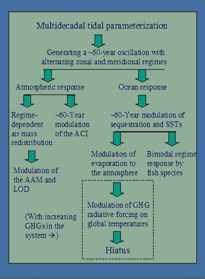
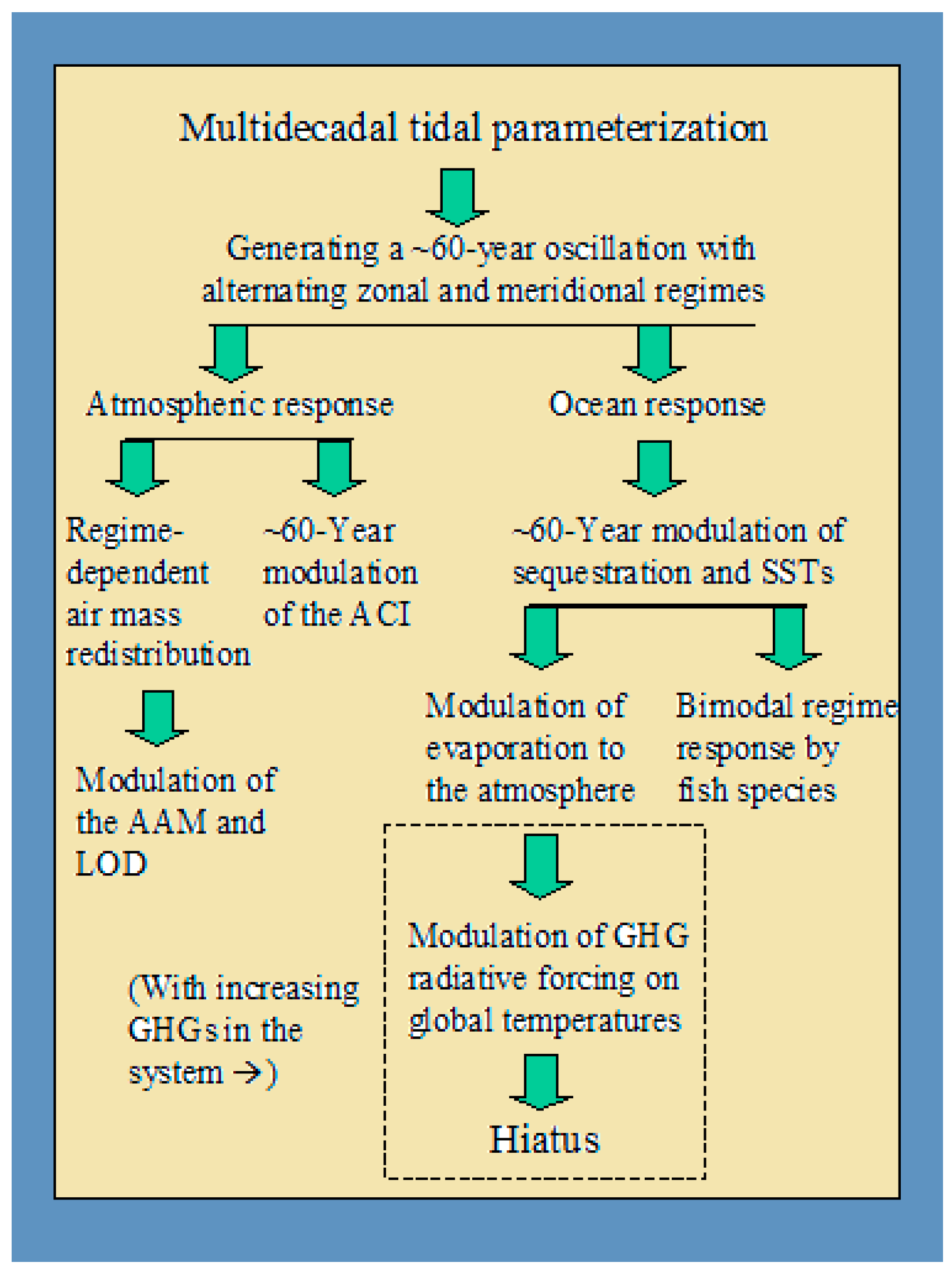
Controversy has surrounded some of these issues in climate, geophysics and fisheries biology including the hiatus, the issue at the focus of this paper. As mentioned at the end of Section 1.2, this may be largely due to a need for some physical agent to drive the process. Figure 8 is a schematic amplification of part of a figure in T17, collating the suggested multidecadal scale physical linkages proposed in this paper.
Figure 8 outlines the progression of the tidal treatment to an explanation of the hiatus and other climate-related phenomena. With the exception of the items in the dashed box, the Figure shows components that are hypothesized to be modulated by a ~60-year oscillation, in the absence of increasing amounts of atmospheric greenhouse gases. This is intended to describe the background result of tidal forcing with mid-19th century levels of GHGs, for a preliminary general circulation model (GCM) test of temporal variability. Adding increasing GHGs (in the box) to the system is then hypothesized to produce the hiatus periods when temporal variability is tested with a GCM.
The need for a thorough-going analysis of these implied dynamics was emphasized by Treloar [37]-which was beyond both the scope of that paper and the tools available to the author. There are a limited number of such GCMs incorporating tidal forcing and (to the author’s knowledge) apparently with oscillations only on semidiurnal and diurnal (for example [61] and [62]) rather than multidecadal timescales. It is hoped that a GCM test of the parameterization would examine as much as possible of the causal chain suggested in Figure 8 and in the text and determine if the relevant atmosphere and ocean data on the multidecadal scale can be reproduced.
This paper suggests that the tidal multidecadal components identified in T02, with their defined periods and phases, are present in Pacific and Atlantic ocean basins as well as simulating hiatus periods in the GMST Oscillation 1 component. This supports the linkage between the GMST hiatus phenomenon and cool episodes in these ocean basins noted by previous workers and is consistent with the hypothesis that exogenous tidal forcing is a common ultimate cause. Evidence of bidecadal and shorter period tidal components in ocean oscillations noted above and in T17 suggests the future possibility of a clearer higher frequency characterization of those oscillations. The tidal formulations suggest that bidecadal components would generate hiatus periods with durations around 11 years and contribute, with ~30-year hiatus periods from the ~60-year component, to global and ocean basin temperature temporal variability.
A note of caution might be added about detrended oscillations in ocean basin temperature data. If ocean basin data treatment includes the detrending (implicitly or explicitly) of global warming since approximately 1850, that process may include removing the ~60-year oscillation. It seems likely that most of the multi-century paleoclimate data discussed in this paper would not have been warming-detrended but data treated with dipole/tripole or principal components analysis (such as by Gedalof et al. [48]) and ocean basin data sets beginning from about 1850, may have been. The relatively small contribution of the zonal 59.75-year component in regression analyses of ocean basins noted above may be due not only to the basin oscillations’ general meridional character but also to partial removal of ~60-year oscillations by detrending. In order to delineate the physical parameters underlying ocean basin surface temperature variability, there may be a case for preferring the analysis of unfiltered and undetrended temperature data.
Nevertheless, multidecadal components from the tidal parameterization may be a missing factor in the climate modelling of (a) hiatus periods in the instrumental record of global temperatures and (b) the presence and timing of cool episodes in ocean basins. In this tidal hypothesis, the ~60-year GMST oscillation and ~30-year hiatus periods are a result of a dominant 59.75-year zonal tidal oscillation that is modulated by lower-amplitude 86.81- and 186.0-year meridional components. However, the IPO proxy record of Vance et al. [46] and the variation in significance between the three multidecadal tidal components over different ocean basins indicate that the timing and duration of warmer and cooler periods may depend on latitude or at least on region; ~30-year hiatus periods would not be expected in basins where the 59.75-year zonal component does not dominate.
Many of the articles reviewed by Lewandosky [1] assumed the recent hiatus to commence around 1998, the occasion of a strong El Niño. It seems noteworthy that the review reported no cases with hiatus end dates of 2011 or 2014, perhaps reflecting the presence of El Niños in 2009/10 and 2014/15/16. At time of writing (January 2019) there is a prospect of another developing El Niño [63]. It seems likely that these assignments of hiatus onset, termination and duration have been significantly influenced by the timing of El Niño events and it may be misleading to assess features such as the hiatus in terms of ENSO-scale events unless there is a physical reason to associate the latter with the beginning or end of the former. As this paper was being revised, a new paper [64] examined the most recent fluctuation and concluded that the reality of this pause is unsupported by robust statistical analysis. As above, that analysis noted the effect of ENSO events blurring the identification, timing and substantiation of the hiatus. As also noted above, rising temperatures from radiative forcing from increasing atmospheric GHGs inevitably tend to obscure a hiatus episode in the noise. However, the present paper is not chiefly focused on the current (or recent) hiatus but rather on outlining a possible mechanism to explain that hiatus in the context of two previous occurrences. The tidal parameterization suggests that hiatus periods in GMSTs do not imply that GHG radiative response has been discontinuous but rather that a steady rise in the radiative effect of GHG forcing has been accompanied by a natural oscillation that has added hiatus periods to that steady rise.
It is proposed (Section 3.2) that the current meridional epoch will last until 2034. The years following the anticipated 2018/19 El Niño will determine whether GMSTs show a resumption of the hiatus or be overridden by the continuing increase in radiative forcing from rising atmospheric GHG concentrations. In any event, it is likely that the latter process will ensure that future meridional circulation regimes will fail to correspond to GMST cooling intervals (similar to a point made by Kosaka and Xie [6]) but that those regimes would nevertheless show smaller GMST increases than the zonal regimes that would follow.
Funding
This research received no external funding.
Acknowledgments
Grateful thanks are offered to Ze’ev Gedalof for allowing the use of his SSA analysis of PDO proxy data and to the Department of Atmospheric Sciences at the University of Illinois at Urbana-Champagne, on behalf of the late Michael Schlesinger, for permission to reproduce Schlesinger’s figure as 2b in the text. This paper appears due to support and encouragement from Greg McKeon AM, to whom much is owed.
Conflicts of Interest
The author declares no conflict of interest.
Abbreviations
Glossary of acronyms and symbols used in this paper:
| AAM | atmospheric angular momentum |
| ACI | atmospheric circulation index (Klyashtorin [20]) |
| AMO | Atlantic Multidecadal Oscillation |
| AGW | anthropogenic global warming |
| AMOC | Atlantic Meridional Overturning Oscillation |
| CMIP5 | the Coupled Model Intercomparison Project Phase 5 |
| δ18O | a measure of the ratio of oxygen-18 and oxygen-16 isotopes |
| DT | decision tree (Vance et al.), an independent nonlinear multivariate regression technique |
| ENSO | El Niño-Southern Oscillation |
| GCM | general circulation model |
| GHG | greenhouse gas |
| GMST | global mean surface temperature |
| HadCRUT4 | Hadley Centre Climate Research Unit version 4 global temperature data set |
| IPCC AR5 | United Nations Intergovernmental Panel on Climate Change Fifth Assessment Report |
| IPO | Interdecadal Pacific Oscillation |
| LOD | length of day |
| NAO | North Atlantic Oscillation |
| PDO | Pacific Decadal Oscillation |
| PLF | piece-wise linear fit (Vance et al.), an independent nonlinear multivariate regression technique |
| POGA | Pacific Ocean-Global Atmosphere experiment |
| SST | sea surface temperature |
| T02 | Treloar 2002 paper [36] |
| T17 | Treloar 2017 paper [37] |
| TW | terawatts |
| Z–M | zonal minus meridional (calculation), after Klyashtorin [20] |
References
- Lewandowsky, S.; Risbey, J.S.; Oreskes, N. On the definition and identifiability of the alleged “hiatus” in global warming. Sci. Rep. 2015. [Google Scholar] [CrossRef] [PubMed]
- Trenberth, K.E.; Fasullo, T. An apparent hiatus in global warming? Earth’s Future 2013, 1, 19–32. [Google Scholar] [CrossRef] [Green Version]
- Meehl, G.A.; Arblaster, J.M.; Fasullo, J.T.; Hu, A.; Trenberth, K.E. Model-based evidence of deep-ocean heat uptake during surface temperature hiatus periods. Nat. Clim. Chang. 2011, 1, 360–364. [Google Scholar] [CrossRef]
- Yan, X.-H.; Boyer, T.; Trenberth, K.; Karl, T.R.; Xie, S.-P.; Nieves, V.; Tung, K.-K.; Roemmich, D. The global warming hiatus: Slowdown or redistribution? Earth’s Future 2016, 4, 472–482. [Google Scholar] [CrossRef] [Green Version]
- Drijfhout, S.S.; Blaker, A.T.; Josey, S.A.; Nurser, A.J.G.; Sinha, B.; Balmaseda, M.A. Surface warming hiatus caused by increased heat uptake across multiple ocean basins. Geophys. Res. Lett. 2014, 41, 7868–7874. [Google Scholar] [CrossRef] [Green Version]
- Kosaka, Y.; Xie, S.-P. Recent global warming hiatus tied to equatorial Pacific surface cooling. Nature 2013, 501, 403–407. [Google Scholar] [CrossRef] [PubMed]
- Kosaka, Y.; Xie, S.-P. The tropical Pacific as a key pacemaker of the variable rates of global warming. Nat. Geosci. 2016, 9, 669–673. [Google Scholar] [CrossRef]
- von Känel, L.; Fröhlicher, T.L.; Gruber, N. Hiatus-like decades in the absence of equatorial Pacific cooling and accelerated global ocean uptake. Geophy. Res. Lett. 2017, 44, 7909–7918. [Google Scholar] [CrossRef]
- Trenberth, K.E. Has there been a hiatus? Science 2015, 349, 691–692. [Google Scholar] [CrossRef] [Green Version]
- Yao, S.-L.; Huang, G.; Wu, R.-G.; Qu, X. The global warming hiatus–A natural product of interactions of a secular warming trend and a multi-decadal oscillation. Theor. Appl. Climatol. 2016, 123, 349–360. [Google Scholar] [CrossRef]
- Brown, P.T.; Li, W.; Xie, S.P. Regions of significant influence on unforced global mean surface air temperature variability in climate models. J. Geophys. Res. Atmos. 2014, 120, 480–494. [Google Scholar] [CrossRef]
- Meehl, G.A.; Arblaster, J.M.; Bitz, C.M.; Chung, T.Y.; Teng, H. Antarctic sea-ice expansion between 2000 and 2014 driven by tropical Pacific decadal climate variability. Nat. Geosci. 2016, 9, 590–595. [Google Scholar] [CrossRef]
- Kincer, J.B. Our changing climate. Eos Trans. AGU 1946, 27, 342–347. [Google Scholar] [CrossRef]
- Wigley, T.M.L.; Angell, J.K.; Jones, P.D. Analysis of the temperature record. In Detecting the Climatic Effects of Increasing Carbon Dioxide; MacCracken, M.C., Luther, F.M., Eds.; (DOE/ER-0235); U.S. Department of Energy, Carbon Dioxide Research Division: Washington, DC, USA, 1985; pp. 55–90. [Google Scholar]
- Easterling, D.R.; Wehner, M.F. Is the climate warming or cooling? Geophys. Res. Lett. 2009, 36. [Google Scholar] [CrossRef] [Green Version]
- Lovejoy, S. Return periods of global climate fluctuations and the pause. Geophys. Res. Lett. 2014, 41. [Google Scholar] [CrossRef]
- England, M.H.; McGregor, S.; Spence, P.; Meehl, G.A.; Timmerman, A.; Cai, W.; Gupta, A.S.; McPhaden, M.J.; Purich, A.; Santoso, A. Recent intensification of wind-driven circulation in the Pacific and the ongoing warming hiatus. Nat. Clim. Chang. 2014, 4, 222–227. [Google Scholar] [CrossRef] [Green Version]
- Schlesinger, M.E.; Ramankutty, N. An oscillation in the global climate system of period 65–70 years. Nature 1994, 367, 723–726. [Google Scholar] [CrossRef]
- Schlesinger, M.E.; Lindner, D.; Ring, M.J.; Cross, E.F. A simple deconstruction of the HADCRU global-mean near-surface temperature observations. Atmos. Clim. Sci. 2013, 3, 348–354. [Google Scholar] [CrossRef]
- Klyashtorin, L.B. Climate Change and Long-Term Fluctuations of Commercial Catches: The Possibility of Forecasting; UN FAO Fisheries Technical Paper 410; Food and Agriculture Organization of the United Nations: Rome, Italy, 2001. [Google Scholar]
- Mann, K.; Lazier, J.R.N. Variability in ocean circulation: Its biological consequences. In Dynamics of Marine Ecosystems: Biological-Physical Interactions in the Oceans, 3rd ed.; Wiley-Blackwell: Hoboken, NJ, USA, 2006. [Google Scholar]
- Oviatt, C.; Smith, L.; McManus, M.C.; Hyde, K. Decadal patterns of westerly winds, temperatures, ocean gyre circulations and fish abundance: A review. Climate 2015, 3, 833–857. [Google Scholar] [CrossRef]
- Knight, J.R.; Allan, R.J.; Folland, C.K.; Vellinga, M.; Mann, M.E. A signature of persistent natural thermohaline circulation cycles in observed climate. Geophys. Res. Lett. 2005, 32, 475–480. [Google Scholar] [CrossRef]
- Mann, M.E.; Bradley, R.S.; Hughes, M.K. Global-scale temperature patterns and climate forcing over the last six centuries. Nature 1998, 392, 779–787. [Google Scholar] [CrossRef]
- Delworth, T.L.; Mann, M.E. Observed and simulated multidecadal variability in the Northern Hemisphere. Clim. Dyn. 2000, 16, 661–676. [Google Scholar] [CrossRef]
- Chambers, D.P.; Merrifield, M.A.; Nerem, R.S. Is there a 60-year oscillation in global sea level? Geophys. Res. Lett. 2012, 39, L18607. [Google Scholar] [CrossRef]
- Moore, G.W.K.; Halfar, J.; Majeed, H.; Adey, W.; Kronz, A. Amplification of the Atlantic Multidecadal Oscillation associated with the onset of the industrial-era warming. Nat. Sci. Rep. 2017, 7. [Google Scholar] [CrossRef] [PubMed]
- Knudsen, M.F.; Seidenkrantz, M.-S.; Jacobsen, B.H.; Kuijpers, A. Tracking the Atlantic Multidecadal Oscillation through the last 8000 years. Nat. Commun. 2011, 2. [Google Scholar] [CrossRef]
- Kilbourne, K.H.; Quinn, T.M.; Webb, R.; Guilderson, T.; Nyberg, J. Paleoclimate proxy perspective on Caribbean climate since the year 1751: Evidence of cooler temperatures and multidecadal variability. Paleoceanography 2008, 23, PA3220. [Google Scholar] [CrossRef]
- Kuhlbrodt, T.; Griesel, A.; Montoya, M.; Levermann, A.; Hofmann, M.; Rahmstorf, S. On the driving processes of the Atlantic Meridional Overturning Circulation. Rev. Geophys. 2007, 45. [Google Scholar] [CrossRef]
- Doodson, A.T. The harmonic development of the tide-generating potential. Proc. R. Soc. A Math. Phys. Eng. Sci. 1921, 100, 305–329. [Google Scholar] [CrossRef]
- Cartwright, D.E.; Taylor, R.J. New computations of the tide generating potential. Geophys. J. R. Astron. Soc. 1971, 23, 45–74. [Google Scholar] [CrossRef]
- Keeling, C.D.; Whorf, T.P. Possible forcing of global temperatures by the oceanic tides. Proc. Natl. Acad. Sci. USA 1997, 94, 8321–8328. [Google Scholar] [CrossRef]
- Keeling, C.D.; Whorf, T.P. The 1800-year oceanic tidal cycle: A possible cause of rapid climate change. Proc. Natl. Acad. Sci. USA 2000, 97, 3814–3819. [Google Scholar] [CrossRef] [PubMed]
- Munk, W.H.; Wunsch, C. Abyssal recipes II: Energetics of tidal and wind mixing. Deep Sea Res. I 1998, 45, 1977–2010. [Google Scholar] [CrossRef]
- Treloar, N.C. Luni-solar influences on climate variability. Int. J. Climatol. 2002, 22, 1527–1542. [Google Scholar] [CrossRef]
- Treloar, N.C. Deconstructing global temperature anomalies: An hypothesis. Climate 2017, 5, 83. [Google Scholar] [CrossRef]
- Wood, F.J. Tidal Dynamics: Coastal Flooding, and Cycles of Gravitational Force; D. Reidel: Norwell, MA, USA, 1996. [Google Scholar]
- Schlesinger, M.E. 2016 evaluation of Fair Plan 3: Outlook for global temperature change throughout the 21st century. J. Environ. Prot. 2017, 8, 426–435. [Google Scholar] [CrossRef]
- U.S. Climate Change Science Program. Scenarios of Greenhouse Gas Emissions and Atmospheric Concentrations; U.S. Climate Change Science Program: Washington, DC, USA, 2007.
- Lacis, A.A.; Schmidt, G.A.; Rind, D.; Ruedy, R.A. Atmospheric CO2: Principal control knob governing Earth’s temperature. Science 2010, 330, 356–359. [Google Scholar]
- Huang, H.P.; Weickmann, K.M.; Hsu, C.J. Trend in atmospheric angular momentum in a transient climate change simulation with greenhouse gas and aerosol forcing. J. Clim. 2001, 14, 1525–1534. [Google Scholar] [CrossRef]
- Philander, S.G.H. El Niño and the Southern Oscillation; Academic Press: New York, NY, USA, 1990. [Google Scholar]
- Hide, D.; Dickey, J.O. Earth’s variable rotation. Science 1991, 253, 629–637. [Google Scholar] [CrossRef]
- Morice, C.P.; Kennedy, J.J.; Rayner, N.A.; Jones, P.D. Quantifying uncertainties in global and regional temperature change using an ensemble of observational estimates: The HadCRUT4 dataset. J. Geophys. Res. 2012, 117, D08101. [Google Scholar] [CrossRef]
- Vance, T.R.; Roberts, J.L.; Plummer, C.T.; Kiem, A.S.; van Ommen, T.D. Interdecadal Pacific variability and eastern Australian megadroughts over the last millennium. Geophys. Res. Lett. 2014, 42, 129–137. [Google Scholar] [CrossRef]
- MacFarling Meure, C.; Etheridge, D.; Trudinger, C.; Steele, P.; Langenfelds, R.; van Ommen, T.; Smith, A.; Elkins, J. Law Dome CO2, CH4 and N2O ice core record extended to 2000 years BP. Geophys. Res. Lett. 2006, 33, L14810. [Google Scholar] [CrossRef]
- Gedalof, Z.; Mantua, N.; Peterson, D.L. A multi-century perspective of variability in the Pacific Decadal Oscillation: New insights from tree rings and coral. Geophys. Res. Lett. 2002, 29, 2204. [Google Scholar] [CrossRef]
- Kipfmueller, K.F.; Larson, E.R.; St. George, S. Does proxy uncertainty affect the relations inferred between the Pacific Decadal Oscillation and wildfire activity in the western United States? Geophys. Res. Lett. 2012, 39. [Google Scholar] [CrossRef] [Green Version]
- MacDonald, G.M.; Case, R.A. Variations in the Pacific Decadal Oscillation over the past millennium. Geophys. Res. Lett. 2005, 32, L08703. [Google Scholar] [CrossRef]
- Shen, C.; Wang, W.-C.; Gong, W.; Hao, Z. A Pacific Decadal Oscillation record since 1470 AD reconstructed from proxy data of summer rainfall over eastern China. Geophys. Res. Lett. 2006, 33, L03702. [Google Scholar] [CrossRef]
- Henley, B.J.; Gergis, J.; Karoly, D.J.; Power, S.B.; Kennedy, J.; Folland, C.K. A tripole index for the Interdecadal Pacific Oscillation. Clim. Dyn. 2015, 45, 3077–3090. [Google Scholar] [CrossRef]
- National Oceanic and Atmospheric Administration (NOAA). National Centers for Environmental Information (NCEI, formerly National Climatic Data Center, NCDC) PDO Data. Available online: https://www.ncdc.noaa.gov/teleconnections/pdo/data.csv (accessed on 13 December 2018).
- Biondi, F.; Gershunov, A.; Cayan, D.R. North Pacific decadal climate variability since 1661. J. Clim. 2001, 14, 5–10. [Google Scholar] [CrossRef]
- Gedalof, Z.; Smith, D.J. Interdecadal climate variability and regime-scale shifts in Pacific North America. Geophys. Res. Lett. 2001, 28, 1515–1518. [Google Scholar] [CrossRef] [Green Version]
- Jones, P.D.; Jonsson, T.; Wheeler, D.A. Extension to the North Atlantic Oscillation using early instrumental pressure observations from Gibraltar and South-West Iceland. Int. J. Climatol. 1997, 17, 1433–1450. [Google Scholar] [CrossRef]
- Vinther, B.M.; Johnsen, S.J.; Andersen, K.K.; Clausen, H.B.; Hansen, A.W. NAO signal recorded in the stable isotopes of Greenland ice cores. Geophys. Res. Lett. 2003, 30, 1387. [Google Scholar] [CrossRef]
- Luterbacher, J.; Xoplaki, E.; Dietrich, D.; Jones, P.D.; Davies, T.D.; Portis, D.; Gonzalez-Rouco, J.F.; von Storch, H.; Gyalistras, D.; Casty, C.; Wanner, H. Extending North Atlantic Oscillation reconstructions back to 1500. Atmos. Sci. Lett. 2002, 2, 114–124. [Google Scholar] [CrossRef]
- Glueck, M.F.; Stockton, C.W. Reconstruction of the North Atlantic Oscillation, 1429–1983. Int. J. Climatol. 2001, 12, 1453–1465. [Google Scholar] [CrossRef]
- Cook, E.R.; D’Arrigo, R.D.; Mann, M.E. Well Verified Winter North Atlantic Oscillation Index Reconstruction; IGBP PAGES/World Data Center for Paleoclimatology Data Contribution Series #2002-059; NOAA/NGDC Paleoclimatology Program: Boulder CO, USA, 2002.
- Schiller, A.; Fiedler, R. Explicit tidal forcing in an ocean general circulation model. Geophys. Res. Lett. 2007, 34. [Google Scholar] [CrossRef] [Green Version]
- Yu, Y.; Liu, H.; Lan, J. The influence of explicit tidal forcing in a climate circulation model. Acta Oceanol. Sin. 2016, 35, 42–50. [Google Scholar] [CrossRef]
- National Oceanic and Atmospheric Administration (NOAA); National Centers for Environmental Information (NCEI). Global Climate Report for October 2018. Published Online November 2018. Available online: https://www.ncdc.noaa.gov/sotc/global/201810 (accessed on 12 December 2018).
- Lewandowsky, S.; Cowtan, K.; Risbey, J.S.; Mann, M.E.; Steinman, B.A.; Oreskes, N.; Rahmstorf, S. The ‘pause’ in global warming in historical context: (II). Comparing models to observations. Environ. Res. Lett. 2018, 13, 123007. [Google Scholar] [CrossRef]
Figure 1.
Relative contributions of the three multidecadal tidal components, a composite of the three components in T17. The amplitude of the 59.75-year component is 1700 on this scale.
Figure 1.
Relative contributions of the three multidecadal tidal components, a composite of the three components in T17. The amplitude of the 59.75-year component is 1700 on this scale.

Figure 2.
Adding tidal and curvilinear components to simulate annual unsmoothed HadcRUT4 global mean surface temperature (GMST) anomalies, the curves projected to 2040.
Figure 2.
Adding tidal and curvilinear components to simulate annual unsmoothed HadcRUT4 global mean surface temperature (GMST) anomalies, the curves projected to 2040.

Figure 3.
The Z–M sine curve representing tidal contributions to GMST anomalies, with the corresponding cosine curve showing the timing of positive and negative intervals of Z–M values. GMST meridional regimes and hiatus periods are proposed to be defined by falling temperatures in the solid sine curve and by negative segments of the dashed cosine curve.

Figure 4.
Hypothesized multidecadal tidal contribution to GMSTs, according to the variation in the integrated zonal-meridional difference in the tidal parameterization.
Figure 4.
Hypothesized multidecadal tidal contribution to GMSTs, according to the variation in the integrated zonal-meridional difference in the tidal parameterization.

Figure 5.
(a) Three hypothesized tidal oscillations present in GMST anomalies at successively higher frequencies; (b) An equivalent deconstruction by Schlesinger [39], reprinted by kind permission of the Department of Atmospheric Sciences at the University of Illinois at Urbana-Champagne on behalf of the late Michael Schlesinger.

Figure 6.
Comparing the IPO proxy of Vance et al. [46] with two vertically-scaled meridional tidal oscillations.
Figure 6.
Comparing the IPO proxy of Vance et al. [46] with two vertically-scaled meridional tidal oscillations.

Figure 7.
A comparison of derived PDO and tidal components. Blue: PDO eigenvector modes found by Gedalof et al. [48]. Red: Tidal components derived in T02 and T17, vertically scaled. The figures compare respective eigenvector modes and tidal curves having periods: (a) ~23 and 21.70 years; (b) ~20 and 18.60 years; and (c) ~80 or ~85 and 86.81 years. SSA data for the three modes are used by kind permission of Prof. Gedalof.

Figure 8.
Schematic diagram of suggested relationships between some issues in climate, geophysics and fisheries biology that may be interrelated through an exogenous causal agent, tidal forcing.
Figure 8.
Schematic diagram of suggested relationships between some issues in climate, geophysics and fisheries biology that may be interrelated through an exogenous causal agent, tidal forcing.


Table 1.
The probability p-value pattern for the 186.0-, 86.81- and 59.75-year tidal components in regressions of temperature variability in Pacific and Atlantic ocean basins and including the sense (positive or negative) of the correlation. Key: quadruple sign (+ or −), p < 10−10; triple sign, p < 10−5; double sign, p < 0.05; single sign, correlation not significant. N.B. the proxy data for Shen et al. [51] and for MacDonald and Case [50] were linearly detrended before regression.
| Oscillation | Data Source | Data Length (yr), Frequency | 186.0 yr | 86.81 yr | 59.75 yr |
|---|---|---|---|---|---|
| IPO | Vance et al. PLF [DT-median] [46] | 998, yearly | + + + + [+ + + + ] | – – – [– – – –] | + [+ +] |
| IPO-TPI | Henley et al. [52] | 141, monthly | + + | – – – – | + |
| PDO | NOAA / NCEI [53] | 163, monthly | + + | – – | + + + |
| PDO | Shen et al. [51] | 529, yearly | – | + + | + + |
| PDO | Biondi et al. [54] | 331, yearly | – | – | + + |
| PDO | Gedalof et al. [48] | 157, yearly | + + | – – – | + + |
| PDO | Gedalof and Smith [55] | 385, yearly | – | – | – |
| PDO | MacDonald and Case [50] | 1004, yearly | + + | + | + + |
| NAO | Jones et al. [56] | 177, yearly | + | – – – – | + + + |
| NAO | Vinther et al. [57] | 726, yearly | + | – | + + |
| NAO | Luterbacher et al. [58] | 491, yearly | + + | – – | + + |
| NAO | Glueck and Stockton [59] | 525, yearly | + | – – – – | + + |
| NAO | Cook et al. [60] | 580, yearly | + | – – | – |
© 2019 by the author. Licensee MDPI, Basel, Switzerland. This article is an open access article distributed under the terms and conditions of the Creative Commons Attribution (CC BY) license (http://creativecommons.org/licenses/by/4.0/).
Share and Cite
MDPI and ACS Style
Treloar, N.C. A Proposed Exogenous Cause of the Global Temperature Hiatus. Climate 2019, 7, 31. https://doi.org/10.3390/cli7020031
AMA Style
Treloar NC. A Proposed Exogenous Cause of the Global Temperature Hiatus. Climate. 2019; 7(2):31. https://doi.org/10.3390/cli7020031
Chicago/Turabian StyleTreloar, Norman C. 2019. "A Proposed Exogenous Cause of the Global Temperature Hiatus" Climate 7, no. 2: 31. https://doi.org/10.3390/cli7020031
Note that from the first issue of 2016, this journal uses article numbers instead of page numbers. See further details here.