Precipitation Trends over the Indus Basin

Abstract

A large population relies on water input to the Indus basin, yet basinwide precipitation amounts and trends are not well quantified. Gridded precipitation data sets covering different time periods and based on either station observations, satellite remote sensing, or reanalysis were compared with available station observations and analyzed for basinwide precipitation trends. Compared to observations, some data sets tended to greatly underestimate precipitation, while others overestimate it. Additionally, the discrepancies between data set and station precipitation showed significant time trends in many cases, suggesting that the precipitation trends of those data sets were not consistent with station data. Among the data sets considered, the station-based Global Precipitation Climatology Centre (GPCC) gridded data set showed good agreement with observations in terms of mean amount, trend, and spatial and temporal pattern. GPCC had average precipitation of about 500 mm per year over the basin and an increase in mean precipitation of about 15% between 1891 and 2016. For the more recent past, since 1958 or 1979, no significant precipitation trend was seen. Among the remote sensing based data sets, the Tropical Rainfall Measuring Mission Multi-Satellite Precipitation Analysis (TMPA) compared best to station observations and, though available for a shorter time period than station-based data sets such as GPCC, may be especially valuable for parts of the basin without station data. The reanalyses tended to have substantial biases in precipitation mean amount or trend relative to the station data. This assessment of precipitation data set quality and precipitation trends over the Indus basin may be helpful for water planning and management.

1. Introduction

The Indus is the westernmost of the major rivers of South Asia. It has a total length of 3200 km and drains parts of China, India, Afghanistan and Pakistan [1], in particular providing Pakistan’s main water source. The Indus basin’s water resources have been estimated to support 215 million people with an average per capita annual water availability of 1329 m${}^3$ [2]. The Indus originates from Tibetan Plateau and drains into the Arabian Sea, and the basin as a whole covers a latitude range of about 24${}^{\circ }$ to 37${}^{\circ }$ N and longitude range of about 66${}^{\circ }$ to 82${}^{\circ }$ E (Figure 1). The northern or upper part of the basin includes high mountains of the Himalaya, Karakoram, and Hindu Kush mountain ranges, whereas much of its southern or lower part is flat lowland. Temperatures range from below freezing at high elevations to above 40 ${}^{\circ }$C in spring and summer at low elevations. Located at the margin of the South Asia Summer Monsoon region, much of the Indus basin is relatively arid. Particularly the upper part of the basin receives a substantial share of precipitation in winter, during westerly disturbances [3,4,5]. Some 85% of the Indus’ flow is in the summer, when both monsoon rain and mountain glacier melt peak [1,6].

Quantifying historic precipitation change is key for understanding variability and change in the water budget over the Indus basin. Climate model simulations mostly project that anthropogenic global warming would lead to increased precipitation in the region over the coming decades, but decreased snowfall at high elevations in winter and increased evaporation, which could lead to reduced reliability of water resources [7,8]. Moreover, there is high uncertainty owing to divergent behavior of climate models and limited ground observations [9,10,11]. Sparsity and discontinuity of climate and hydrologic observations make it difficult to evaluate the accuracy of hydrologic and climate models and create gaps in the scientific understanding needed to provide evidence for policy decisions [12,13]. Globally, there is recognition of an increased need for employing statistical analyses to provide better information about long-term changes and variability of precipitation as a result of the changing climate and consequent greater exposure to risks such as droughts and floods [14].

Most previous work on precipitation trends in the Indus basin has focused only on portions of the basin, defined by political or hydrologic boundaries. For example, Archer and Fowler [15] examined precipitation records of varying lengths from 17 stations in the Upper Indus basin, and found no significant precipitation trend from 1895–1999 overall, but increases in some stations over the most recent decades of 1961–1999. Bhutiyani et al. [16] examined station precipitation at three stations in Jammu and Kashmir and Himachal Pradesh states, India, finding negative trends in precipitation over 1866–2006. Khattak et al. [17] found no definite pattern in precipitation over the period 1967–2005 over 20 stations in Pakistan’s portion of the Upper Indus basin. Similarly, investigations of station precipitation records in Pakistan’s lower and middle Indus basin [18] and Swat river subbasin [19] found insignificant trends over 40–50 year periods. A study of 53 meteorological stations over the China–Pakistan Economic Corridor during 1980–2016 found mixed trends by season and altitude, with little change in mean precipitation overall and most of the seasonal changes not showing statistical significance [20]. Chevuturi et al. [21] studied trends in precipitation based on station measurements and different gridded data sets at one location, Leh, Jammu and Kashmir, India. Iqbal et al. [22] found no trend in annual precipitation over northern Pakistan using the Asian Precipitation–Highly Resolved Observational Data Integration Towards Evaluation of Water Resources (APHRODITE) gridded precipitation data set for 1951–2007. Using Global Precipitation Climatology Centre (GPCC) gridded data over Pakistan for 1961–2010, Ahmed et al. [23] found that many grid cells over the northern part of the country had increasing trends, but that fewer grid cells had significant increases after adjusting for temporal autocorrelation. Trends in heavy summer monsoon precipitation were also investigated in relation to the devastating 2010 floods in Pakistan [24]. Multi-century hydroclimate variations have been assessed for parts of South Asia using tree-ring and other proxies [25,26]. In the Upper Indus basin, tree rings were used to reconstruct streamflow for the period 1452–2008, showing that flows over the recent 1988–2008 period were historically high and that multi-decade periods of particularly low flow occurred in the 16th and 17th Centuries [27]. Hunt, K.M.R. et al. [28] argued based on simulations with an ensemble of climate models that low winter solar insolation in the mid-Holocene led to smaller meridional temperature gradients, a less intense subtropical westerly jet in the midlatitude winter troposphere, and therefore less frequent and intense westerly disturbances over the Indus basin and less winter precipitation, along with more summer precipitation.

In the present work, the main goal is to estimate precipitation amounts and trends over the Indus basin based on available station data. To achieve this, we compared current versions of different global or regional precipitation data sets that cover the basin with generally incomplete available station records within the basin on the monthly timescale. Attention was paid to each data set’s accuracy in representing precipitation totals, seasonal distribution, and interannual variability. In particular, we assessed whether a data set’s precipitation trend is inconsistent with the station measurements, which could manifest as a time-varying bias between the two data sets. Two main timescales were considered for trend estimation: the past 100–150 years, over which station observations have been made, and the past ∼40–60 years, roughly corresponding to the availability of information on precipitation from satellite remote sensing and from global weather observations. Our hypothesis is that careful comparison with available station observations can narrow the range in precipitation amount and trend from that found in different data sets and thus provide more reliable information for assessing climatic change and its hydrologic impacts. The methods developed could also be applied to study trends either in more detail over parts of the Indus basin or in other basins where there is currently high uncertainty.

2. Methods

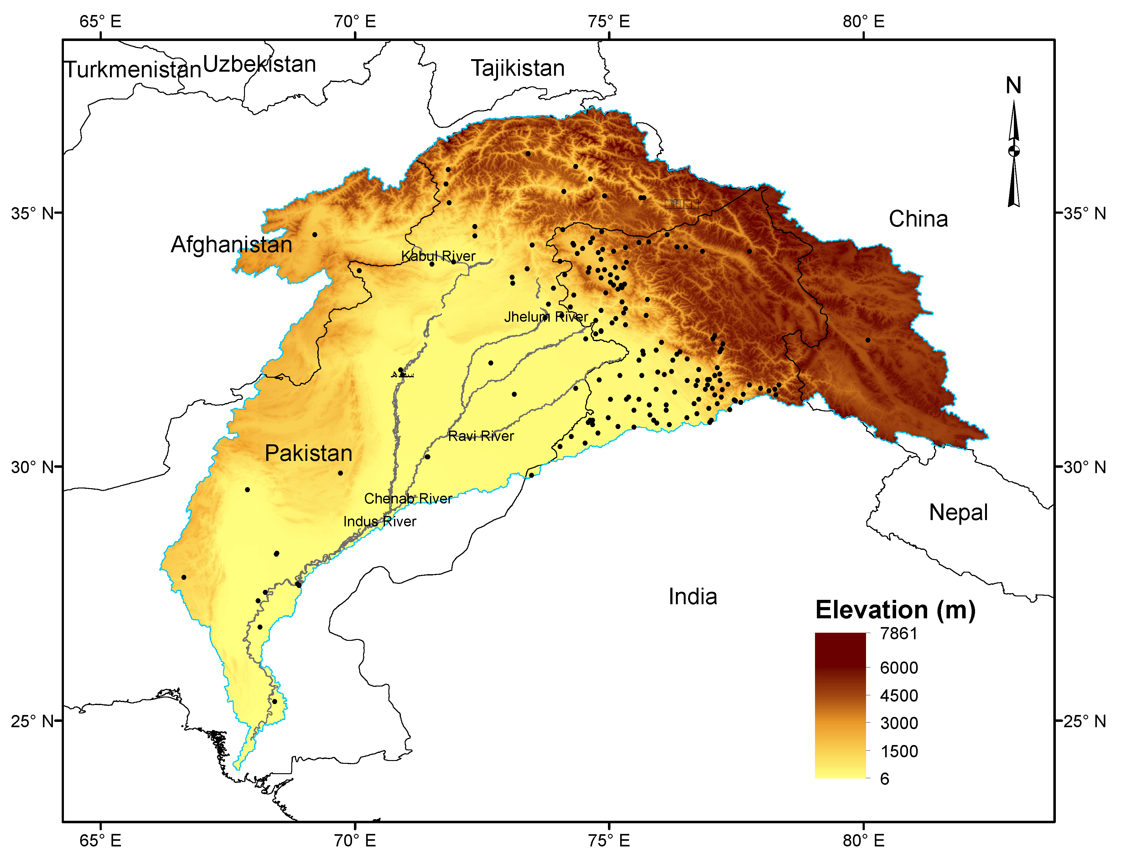
2.1. Basin Delineation

The Indus basin outline was derived from Hydrological Data and Maps Based on Shuttle Elevation Derivatives at Multiple Scales (HydroSHEDS) [29]. This global data set was based primarily on elevation data obtained during the 2000 Shuttle Radar Topography Mission (SRTM) [30], with extensive manual adjustments intended to yield high-quality basin boundaries. The resulting derived basin area was 864,062 km${}^2$ (Figure 1). Note that there is variation between different sources and authors as to the Indus basin boundaries, particularly in the northeast and southeast margins, where extensive areas appear to have endorheic drainage and no surface water connection to the Indus, although they may contribute groundwater to the river [31].

2.2. Station Precipitation Observations

Station precipitation accumulations at daily or monthly resolution were obtained from three sources:

• Precipitation up to the end of 2018 from all available stations ($n=$ 160) within the Indus basin were extracted from the Global Historical Climatology Network–Daily (GHCN) dataset [32]. The included stations were mostly in India, with some in Pakistan and Afghanistan. Observations went back as far as 1901, with the largest number before 1981. Observations flagged for quality concerns [33] were not used.
• Monthly precipitation for 35 stations in Pakistan, covering primarily the period 1980–2014, was obtained from the Pakistan Meteorological Department (PMD), Government of Pakistan.
• Monthly precipitation amounts for nine stations in Pakistan for 1997–2008 were obtained from the International Water Management Institute (IWMI) online Water Data Portal, with PMD also the ultimate source.

Daily values were summed to obtain monthly ones provided that all days in the month had valid observations. After combining station records that appeared in more than one source, there were a total of 73,344 monthly observations from 186 different stations within the Indus basin (Figure 1).

Because the station observations are sparse and in most cases are not complete over multiyear periods, we did not attempt here to reconstruct the basinwide precipitation by year or its trends based on the station observations directly. Instead, we used the station observations to check the consistency of precipitation distribution and trends given by different gridded precipitation data sets in order to indirectly evaluate data sets’ biases and determine which ones give plausible precipitation trends.

2.3. Gridded Precipitation Data Sets

2.3.1. Overview

Broadly, three types of gridded precipitation data sets were considered here for the Indus basin: station-based data sets, satellite-based data sets, and reanalyses. We attempted to choose state-of-the-art precipitation data sets, especially those which covered a long time period or had relatively high spatial resolution. The available temporal coverage and spatial resolution varied between data set types, with station-based data sets, for example, spanning longer periods (over 100 years) compared to satellite-based data sets, which span no more than 40 years.

Table 1. List of precipitation data sets, their spatial resolution, and years for which they were used. Types are G = station-based gridded, S = satellite-based, R = reanalysis. See text for references and more details for each data set.

Data Set	Type	Resolution	Years
GPCC	G	0.5${}^{\circ }$	1891–2016
CRU	G	0.5${}^{\circ }$	1901–2018
APHRODITE V1101	G	0.25${}^{\circ }$	1951–2007
APHRODITE V1901	G	0.25${}^{\circ }$	1998–2015
GPCP	S	2.5${}^{\circ }$	1979–2018
TMPA	S	0.25${}^{\circ }$	1998–2018
IMERG	S	0.1${}^{\circ }$	2015–2018
JRA-55	R	0.5625${}^{\circ }$	1958–2013
MERRA-2	R	0.625${}^{\circ }$× 0.5${}^{\circ }$	1980–2018
ERA5	R	0.5${}^{\circ }$	1979–2018
20CR-2c	R	1.875${}^{\circ }$	1851–2014
CERA-20C	R	1.125${}^{\circ }$	1901–2010

provides a summary list of the data sets used.

Station-based gridded data sets rely on interpolation to estimate precipitation over areas and times with missing station observations. They may incorporate station observations that are not publicly available, and attempt to adjust for missing data and changing observation practices to estimate precipitation patterns and trends as well as possible.

Satellite remote sensing can detect and quantify precipitation with spatial uniformity compared to uneven gauge networks, and enables truly global data sets with coverage over ocean as well as land [34]. On the other hand, satellite data sets use gauge-based datasets for calibration, so they cannot be regarded as completely independent of ground observations [35].

Reanalyses estimate the past climate state, including precipitation rate, by assimilating various types of observational data in a numerical weather prediction model framework. Here, we examined precipitation patterns and trends over the Indus basin for three state-of-the-art reanalysis data sets that cover recent decades and assimilate a broad range of observational data, plus two long-term reanalyses intended for studying centennial-scale climate changes.

2.3.2. Station-Based Gridded Data Sets

The GPCC V2018 Full Data Monthly Product [36], extending from 1891 to 2016, was obtained at a resolution of 0.5${}^{\circ }$. This is based on data from over 75,000 stations globally and includes extensive quality control and weather-dependent corrections for gauge undercatch, and showed no long-term global precipitation trend overall [37]. GPCC interpolated station data to a uniform grid using a modification of the angular distance weighting method SPHEREMAP [38]. Over the 336 0.5${}^{\circ }$ grid cells in the Indus basin, the number of stations used in GPCC increased from about 60 at the beginning of the data set to about 130 in the 1960s, then gradually declined to about 30 in recent years, which parallels global temporal trends in the number of available precipitation stations [37].

The University of East Anglia Climate Research Unit (CRU) TS v. 4.03 data set includes monthly precipitation as well as other weather variables at 0.5${}^{\circ }$ resolution [39] for 1901–2018. It uses fewer stations than GPCC globally, under 10,000; nevertheless, precipitation trends over large regions are similar to those found using GPCC [39]. For the Indus basin, the number of stations used ranged from about 10 at the beginning and end of the coverage period to about 20 in the 1960s through 1980s.

Asian Precipitation–Highly Resolved Observational Data Integration Towards Evaluation of Water Resources (APHRODITE) is a set of regional gridded daily data sets available at 0.25${}^{\circ }$ resolution [40]. We used the Monsoon Asia subset in two versions: V1101, which covers the period 1951–2007, and the newer V1901, which uses satellite precipitation retrievals to decide whether to accept extreme values and covers 1998–2015. This is based on data from more stations in the Indus basin than the other station-based data sets, about 130 for V1101 in 1965 and about 90 for V1901 in 2010.

2.3.3. Satellite-Based Gridded Data Sets

The Global Precipitation Climatology Project (GPCP) Version 2.3 Monthly analysis has coarse spatial resolution (2.5${}^{\circ }$) but relatively long spatial coverage (since 1979). The global value shows a small positive trend for 1979–2017 [41]. It merges the GPCC gauge-based values where station observations are available with satellite-based estimates.

The Tropical Rainfall Measuring Mission Multi-Satellite (TRMM) Precipitation Analysis (TMPA) 3B43 version 7 has 0.25${}^{\circ }$ spatial resolution and is available from 1998 quasi-globally (equatorward of 50${}^{\circ }$). Precipitation amounts are calculated based on a combination of microwave and infrared satellite sensors, and the satellite-based estimate is merged with gauge data using an inverse–error–variance weighting [42,43]. TMPA data sets have been evaluated in many parts of the world, including South Asia, with generally favorable results [44,45,46,47,48,49,50].

The Global Precipitation Measurement (GPM) Integrated Multi-satellite Retrievals for GPM (IMERG) data set is intended to be an eventual successor to TMPA that uses the advanced capabilities of the GPM precipitation radar launched in 2014 [51]. It has a higher resolution of 0.1${}^{\circ }$ and global coverage. We used IMERG V06 Research/Final Run data set, currently available only beginning March 2014, for 2015–2018. Initial work has found IMERG to outperform TMPA over catchments in northern Pakistan [52], southeastern China [53,54], and in the southern Tibetan Plateau [55], as well as in other regions [56,57,58].

2.3.4. Reanalyses

The 55-year Japan Meteorological Agency Reanalysis (JRA-55) was based on an operational weather prediction model and data assimilation system and assimilated surface, upper air and satellite measurements for the period 1958 to 2013. It overcame many of the biases of the previous JRA-25 and other earlier reanalyses and featured realistic precipitation interannual variability and trends, although it did not assimilate surface precipitation observations and overestimated precipitation over the tropics [59,60].

The Modern-Era Retrospective analysis for Research and Applications (MERRA) was intended to utilize satellite observations and improve representation of the hydrologic cycle [61]. The current MERRA-2 further incorporated assimilation of aerosol data and of station precipitation observations [62,63], which has led to it being used extensively for studies of wind and solar availability [64,65,66] as well as in studies of global hydrology [67]. The station precipitation data assimilated into MERRA-2 in the Indus basin region are from the Climate Prediction Center Unified Gauge-Based Analysis of Global Daily Precipitation (CPCU) [63]. CPCU is available in near real time, but, like CRU, uses a small number of stations compared to GPCC: about 16,000 globally, of which over half are in the continental United States [68]. We used MERRA monthly precipitation totals, available since 1980 at a resolution of 0.625${}^{\circ }$ longitude by 0.5${}^{\circ }$ latitude.

The fifth-generation European Centre for Medium-Range Weather Forecasts (ECMWF) Reanalysis (ERA5) replaces the earlier ERA-Interim [69], featuring higher spatial and temporal resolution as well as an improved physical model and data assimilation, and was available beginning from 1979 (planned to extend back to 1950). It has shown better performance compared to previous reanalyses in wind and solar simulation [70,71] as well as in simulating land surface processes [72]. We used output at 0.5${}^{\circ }$ resolution, with the average of a 10-member ensemble is taken to represent the precipitation estimate from this reanalysis.

The 20th Century Reanalysis (20CR) assimilated only surface pressure reports, with observation-based sea-surface temperature and sea ice distributions as boundary conditions, to attempt to supply a consistent estimate of weather dynamics and their evolution over the century [73]. Version 2c (20CR-2c), used here, used more pressure data and more consistent ocean boundary conditions [74]. It had a resolution of about 1.875${}^{\circ }$ and covered the period 1851–2014, thus having the lowest spatial resolution of the reanalyses considered but spanning the longest period. The precipitation data are the average over a 56-member ensemble.

The ECMWF’s Coupled Ocean-Atmosphere 20th Century Reanalysis (CERA-20C) is similar to 20CR in that a restricted set of observations, excluding upper-air and satellite sensors, was assimilated, with the difference that ocean and atmosphere states were assimilated together in a coupled model system [75]. Output was available over 1901–2010 on a reduced Gaussian grid with 1.125${}^{\circ }$ resolution at the Equator, and the average of 10 ensemble members was taken.

2.4. Evaluation of Gridded Precipitation Data Sets

The primary metric chosen for the degree to which each gridded precipitation data set reproduces station observations of monthly precipitation was Nash–Sutcliffe efficiency NSE, which is based on the magnitude of the residual variance relative to the variance of the station observations [76,77,78]:

$$\mathrm{NSE}=1-\frac{\langle {(P_1-P_2)}^2\rangle }{\langle {(P_1-\langle P_1\rangle )}^2\rangle }.$$

(1)

Here, $P_1$ refers to station observations and $P_2$ to a precipitation data set (for the same month as the station observation and evaluated at the grid cell containing the station), and $\langle ·\rangle$ denotes average across observation stations and months. The maximum possible value of NSE is 1, which would obtain if the data set agrees exactly with station observations.

The station observations measure precipitation over the small area of a rain gauge, whereas the gridded precipitation data sets nominally represent precipitation averaged over a much larger grid cell that includes the rain gauge location. Thus, we do not expect perfect correspondence ($\mathrm{NSE}=1$) between the station observations and any of the precipitation data sets. Nevertheless, the degree to which the different data sets approach the station-measured precipitation, as measured by NSE, is expected to offer a reasonable measure of their relative quality.

We considered forms of NSE intended to indicate the performance of the gridded precipitation data sets in representing different aspects of the precipitation observations. These are detailed in Krakauer et al. [77]. Briefly, $\mathrm{NSE}\_all$ compares the original station measurements with the values for the corresponding month and grid point in the precipitation data set. $\mathrm{NSE}\_mean$ compares only the mean annual precipitation values for each station. $\mathrm{NSE}\_seasonal$ compares the mean annual cycle for each station, formed by averaging monthly precipitation amounts across years and then dividing by the annual mean. $\mathrm{NSE}\_variability$ compares the interannual variability in precipitation after the mean annual cycle has been subtracted from each station’s precipitation time series.

Bias in the mean precipitation amount was also computed, as $\mathrm{Bias}=\langle P_2\rangle -\langle P_1\rangle ,$ expressed as a fraction via ${\mathrm{Bias}}_{\mathrm{fractional}}=\frac{\mathrm{Bias}}{\langle P_1\rangle }-1.$

2.5. Precipitation Trends

Basinwide precipitation for each data set and year was computed as an area-weighted average over all grid cells of the data set whose centers are in the basin. Trends in precipitation over the Indus basin for each data set were quantified using least-squares linear regression of the annual amounts over the coverage period of the data set (Table 1), with $p=0.05$ taken to be the threshold for considering a trend to be significantly greater than zero. Trends were also computed using the non-parametric Sen slope method [79] and the Mann–Kendall test (with or without the Hamed and Rao [80] modification for time series autocorrelation) for significance, but the estimated trends and significance levels tended to be quite similar, suggesting that non-normality and serial dependence are not important considerations for regression analysis of the basinwide annual precipitation.

To assess whether the trend in each data set was consistent with available station observations, mean bias was computed for each year, and the trend in the bias time series was checked for significance. If the data set bias varies with time, the data set’s trend is called into question as inconsistent with the available observations. We plotted annual-precipitation time series and calculated correlations in interannual variability of Indus basin precipitation between data sets. We also visualized precipitation trends for selected data sets by location and season to learn more about the inferred trends, although the main focus of this paper is on basinwide annual mean precipitation trends.

3. Results

3.1. Comparison of Gridded Data Sets with Station Observations

The quantitative comparison of the gridded data sets with the available station observations that overlap with their respective periods of availability is summarized in

Table 2. Evaluation of precipitation data sets against station observations.

Data Set	$\mathbf{Bias}\_\mathbf{fractional}$ (%)	$\mathrm{NSE}\_\mathit{all}$	$\mathrm{NSE}\_\mathit{mean}$	$\mathrm{NSE}\_\mathit{seasonal}$	$\mathrm{NSE}\_\mathit{variability}$
GPCC	3	0.804	0.762	0.906	0.704
CRU	−26	0.412	0.157	0.748	0.238
APHRODITE V1101	−14	0.799	0.744	0.941	0.659
APHRODITE V1901	−1	0.718	0.892	0.872	0.448
GPCP	−11	0.610	0.597	0.831	0.464
TMPA	1	0.803	0.900	0.873	0.649
IMERG	12	0.766	0.626	0.515	0.431
JRA-55	26	0.192	−0.002	0.680	−0.130
MERRA-2	−43	0.454	0.326	0.538	0.290
ERA5	19	0.561	0.446	0.801	0.348
20CR-2c	−11	0.055	0.084	0.354	−0.550
CERA-20C	9	0.349	0.236	0.655	0.020

. In terms of mean amount, GPCC and TMPA both performed very well, with fractional biases of under 5% in absolute value. APHRODITE V1101 had precipitation amounts that are some 14% lower than the station observations. This is a very similar bias to that found for this data set by earlier studies in Nepal [77] and High Mountain Asia [81]. APHRODITE V1901 corrected this low bias. CRU and MERRA-2, despite interpolating or assimilating station precipitation observations, underestimated precipitation amount the most compared to station data, possibly due to too few stations from the Indus basin included in these data sets. JRA-55 precipitation was biased high by 26% and ERA5 precipitation was biased high by 19%. The long-term ECMWF reanalysis CERA-20C and the new IMERG satellite data set both had high biases of around 10%, while the 20CR-2c long-term reanalysis and GPCP had a low bias of similar size.

In terms of NSE, GPCC and TMPA performed best overall (highest $\mathrm{NSE}\_all$), followed closely by APHRODITE V1101. APHRODITE V1901 did not improve in $\mathrm{NSE}\_all$ over V1101, although its reduced bias led to improved $\mathrm{NSE}\_mean.$ CRU had the worst correspondence to station observations out of the station-based gridded data sets considered. IMERG performed comparably to GPCP, despite its high bias, which adversely affected especially its $\mathrm{NSE}\_mean$, while GPCP had lower $\mathrm{NSE}\_all.$ Out of the reanalyses, ERA5 outperformed MERRA-2 and JRA-55 and also the long-term reanalyses, among which CERA-20C outperformed 20CR-2c.

The seasonal cycle of precipitation was best represented (as evaluated by $\mathrm{NSE}\_seasonal$) by APHRODITE (especially V1101), followed by GPCC and TMPA. Interannual variability in precipitation ($\mathrm{NSE}\_variability$) was also best represented by GPCC, APHRODITE V1101, and TMPA, with CRU doing particularly poorly for a station-based data set.

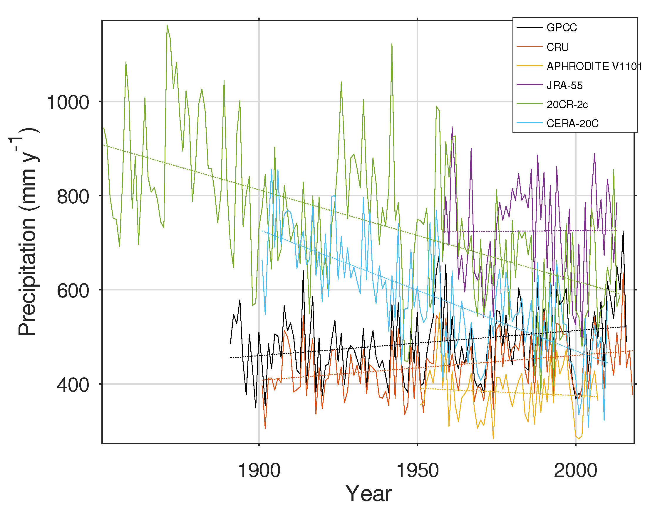
3.2. Trends in Basin Precipitation

Basin-mean precipitation amounts varied by a factor of 2.7 between data sets, ranging from 280 mm y${}^{-1}$ for MERRA-2 to 749 mm y${}^{-1}$ for 20CR-2c (

Table 3. Mean and linear trend for the precipitation data sets over the Indus basin. Units are mm y${}^{-1}$ for mean precipitation and mm y${}^{-2}$ for trends. Trend standard errors are given. * indicates that trends are significantly different from zero at $p<0.05$; ** indicates $p<0.01$. Trends are computed for the available period of each data set (given in Table 1) and, if available, for the uniform 1958–2010 period.

Data Set	Mean	Trend	Bias Trend	Trend (1958–2010)
GPCC	488	+0.53 ± 0.18 **	−1.46 ± 0.80	+0.66 ± 0.69
CRU	439	+0.53 ± 0.16 **	+1.85 ± 0.80 *	+0.54 ± 0.51
APHRODITE V1101	382	−0.31 ± 0.44	+3.21 ± 3.39
APHRODITE V1901	493	+24.45 ± 5.68 **	+19.16 ± 6.07 **
GPCP	580	−0.68 ± 1.18	+8.27 ± 1.14 **
TMPA	503	+6.03 ± 2.74 *	+3.49 ± 1.21 **
IMERG	523	−85.99 ± 34.69	−7.72 ± 34.55
JRA-55	725	+0.07 ± 0.91	+1.52 ± 2.92	−0.02 ± 1.00
MERRA-2	280	+1.28 ± 1.03	+4.57 ± 1.44 **
ERA5	696	−1.91 ± 1.03	+4.71 ± 1.51 **
20CR-2c	749	−1.94 ± 0.21 **	−4.79 ± 1.10 **	−3.89 ± 0.99 **
CERA-20C	585	−2.57 ± 0.25 **	−7.78 ± 1.06 **	−0.92 ± 0.75

). GPCC, TMPA, and APHRODITE V1901, which had among the smallest biases and best overall matches to station observations (Table 2), were, however, in close agreement on a precipitation mean in the middle of this range, around 500 mm y${}^{-1}$.

The long-term observation-based data sets GPCC and CRU both showed a significant positive linear trend over the past ∼120 years (Table 3). The magnitude of this trend, according to GPCC, amounted to an increase in basin-mean precipitation of ∼66 ± 23 mm y${}^{-1}$, or ∼15 ± 5 %, going from ∼455 to ∼521 mm y${}^{-1}$ over the period 1891–2016. GPCC’s bias relative to station observations had no significant linear time trend, which supports the hypothesis that this precipitation trend is real.

JRA-55 showed no significant temporal trend over 1958–2013, and was the only reanalysis data set not to have significant time variation in the mean bias. The long-term reanalyses, by contrast, showed large negative linear trends, which amounted to decreases of ∼35 % (20CR-2c) or ∼39 % (CERA-20C) over the periods of these reanalyses, 1851–2014 and 1901–2010 respectively. However, their bias trend was also significantly negative, suggesting that these negative trends are not consistent with the available station observations.

The shorter-term station and satellite precipitation data sets mostly showed no significant trends. The exceptions were APHRODITE V1901 and TMPA, which both start in 1998 and both showed significant positive trends. However, both these data sets also had significantly positive bias trends, which weakens confidence that their trends are real. Subsetting GPCC showed insignificant positive trends starting in 1951 or 1979 (corresponding to the start dates of different other data sets), but a significant positive trend starting in 1998. Taking 1958–2010 as a common period for many of the station-based and reanalysis data sets, all the available ones showed no significant trend, except for 20CR-2c, which showed a large negative trend that was inconsistent with that found in the other products.

Comparing yearly basin precipitation of GPCC to the long-term reanalyses 20CR-2c and CERA-20C highlighted the contrast in trends between these data sets (Figure 2). Some of the interannual variability in the long-term reanalyses was coherent with that of GPCC, but the reanalyses had consistently too much precipitation, relative to the latter, before ∼1960, and 20CR-2c in particular showed very high year to year variability (Figure 2). For this earlier period, less data may have been available to constrain the reanalyses. GPCC also showed substantial year-to-year variability that was large compared to the long-term precipitation trend. The driest year according to GPCC was 1899, with 349 mm precipitation (most recently, 2002 was almost as dry, with 371 mm), while the wettest was 2015, with 724 mm, or over twice as much.

Table 4. Correlation matrix of the Indus basin mean annual precipitation time series between data sets. The correlation for each pair is based on their period of overlap (Table 1). A = APHRODITE.

	GPCC	CRU	A V1101	A V1901	GPCP	TMPA	IMERG	JRA-55	MERRA-2	ERA5	20CR-2c	CERA-20C
GPCC	1	0.881	0.919	0.872	0.937	0.978	1	0.661	0.656	0.765	0.220	0.360
CRU		1	0.822	0.783	0.831	0.900	0.939	0.702	0.557	0.838	0.168	0.262
A V1101			1	0.946	0.882	0.966	-	0.612	0.452	0.902	0.428	0.706
A V1901				1	0.846	0.846	-	0.703	0.630	0.624	0.092	0.817
GPCP					1	0.984	0.974	0.642	0.560	0.843	0.236	0.840
TMPA						1	0.990	0.842	0.741	0.875	0.223	0.865
IMERG							1	-	0.925	0.790	-	-
JRA-55								1	0.633	0.715	0.391	0.632
MERRA-2									1	0.399	0.304	0.558
ERA5										1	0.315	0.858
20CR-2c											1	0.420
CERA-20C												1

gives the correlations between the different data sets’ basin mean annual precipitation time series, providing a quantitative measure of the extent to which the interannual variability in precipitation visualized in Figure 2 matches. Out of the long-term data sets, GPCC had the highest mean correlation with others. Most of the station and satellite based data sets had correlations above 0.8 with many of the other data sets. 20CR-2c had the worst average correlation with other data sets.

Focusing on GPCC as the best-performing long-term precipitation data set, we examined the trend in precipitation by month. The Indus basin precipitation climatology is bimodal: the major peak in precipitation is in summer (July) with a secondary peak in winter (March), and the corresponding troughs are in November and May (Figure 3, top). The positive precipitation trend for 1891–2016 was significant only for June, October, and November, all climatologically rather dry months. December and January actually showed non-significant decreasing trends (Figure 3, bottom).

Precipitation is quite unevenly distributed over the basin, with mean amounts according to GPCC ranging from 37 to 2399 mm y${}^{-1}$. Precipitation peaks on the southern slopes of the western Himalaya and Karakoram ranges, with low values in the rain shadow north of the mountains as well as in much of the low-lying south (Figure 4, top). Trends in precipitation also varied across the basin in GPCC, with significant positive trends concentrated in the basin’s middle reach and to some extent in the rain shadow region of the north, while most of the mountains and south showed no significant trend and a few areas showed significant drying trends (Figure 4, bottom). Overall, based on GPCC, the increase in precipitation was roughly double over areas where most precipitation does not fall during the June–September summer monsoon, compared to areas where it does (20% vs. 10% increase based on linear regression, compared to a basinwide increase of 15%).

4. Discussion

Our comparison of precipitation data sets with station observations over the Indus basin suggests that GPCC is the best-performing long-term data set. Consistent with our study, Ahmed et al. [82] found that, compared with other station-based gridded precipitation data sets, including APHRODITE V1101 and CRU, GPCC was better correlated with station data in arid southwestern Pakistan. Adnan et al. [83] concluded that “GPCC data are very close to real-time station data and hence may be used in the absence of station data in Pakistan”.

The TMPA remote sensing based data set performed comparably well to GPCC, although it only begins in 1998. TMPA could be more accurate than GPCC for areas without stations, such as the high mountains in the far north of the basin, since it can draw on global remote sensing coverage. It also has the advantage of updating more quickly than the GPCC Full Data Product that we investigated.

The new APHRODITE V1901 was shown to be successful at removing the low bias from which APHRODITE V1101 suffered, although its representation of precipitation seasonality and interannual variability was not improved. Similarly, the new IMERG appeared not to perform better than TMPA, despite higher spatial resolution, and suffered from a high bias.

Out of the satellite-period reanalyses, MERRA-2 underestimated precipitation over the Indus basin, whereas the others (JRA-55 and ERA-5) overestimated it. Globally, the assimilation of precipitation observations reduces the MERRA-2 precipitation by almost 30% compared with that simulated by the underlying climate model, with particularly large-amplitude changes over mountain areas, including the Himalayas [63]. While these observation-based corrections were found to reduce precipitation biases globally for MERRA-2, they may worsen errors in places like the Indus basin where the little gauge data available in near real time may not be regionally representative. In fact, a comparison of MERRA-2 precipitation with GPCP found that MERRA-2 generally underestimates precipitation over the Indus basin (and much of adjoining southern Asia) in both winter and summer [63]. It was concluded that “better-quality precipitation products” available in near real time “are needed to improve the land surface precipitation and thus the terrestrial water budget in forthcoming reanalysis datasets” [63]. Until such improved near real-time precipitation products are made available, precipitation climatologies, such as the GPCC Climatology, could at least be used to correct the mean bias in precipitation for areas such as the Indus basin. Another recent study of precipitation products [13] also showed that MERRA-2 tended to have lower precipitation around the Indus watershed than APHRODITE and TMPA, while ERA-5 had higher precipitation, although that study did not evaluate how these products compared to station observations.

GPCC, supported by CRU, showed a significant increase in precipitation over the Indus basin since the end of the 19th Century. The long-term reanalyses showed, by contrast, a large decrease in precipitation over the same period, which was not supported by observations. Ferguson and Villarini [84] showed that the earlier version of 20CR-2c included pronounced artificial inhomogeneities in many grid cells that were consequences of inhomogeneities in the surface pressure data and ocean boundary conditions. Another factor in the poor performance of 20CR-2c in capturing precipitation amounts and trends may be its low spatial resolution compared to the other reanalyses, which would affect the representation of surface properties such as topography, with dramatic consequences on climate simulation in mountainous regions, and would require coarse physical parameterization of atmospheric processes such as convective precipitation [85,86]. We found that the newer CERA-20C performs better than 20CR-2c at matching station precipitation data but shows an equally strong negative precipitation trend, suggesting that its climate trends may also not be reliable in this region. On the other hand, the shorter-term reanalyses that use upper-air and satellite data showed reasonable precipitation trends, despite evidence of some time-dependent bias as well as substantial mean biases.

Several studies have found that, for many high-elevation subwatersheds of the Indus, station-based gridded data sets tend to underestimate precipitation amounts. Glaciers and snow-covered mountain areas are more important contributors to streamflow for the Indus compared to other major South Asian rivers; while on average amounting to no more than a few percent of basinwide precipitation, glacier melt is disproportionally important in providing water for dry seasons and periods [87]. Immerzeel et al. [88] attempted to infer the extent of underestimation using glacier water balance calculations and streamflow data, although uncertainties in other water balance terms make such assessments imprecise. Dahri et al. [89] used precipitation data from high-altitude stations that have not been previously available for inclusion in gridded datasets along with estimates of precipitation over glaciers from water balance studies to refine the estimated precipitation pattern over the upper Indus basin. For example, their study identifies a precipitation maximum in the extreme north of the Indus watershed (the central Karakoram range in the northwest corner of Shyok basin) that is not seen in GPCC (Figure 4, top) or other station-based gridded data sets, presumably due to lack of station data. Particularly with adjustment for gauge undercatch, the improved precipitation climatology was more consistent with measured streamflows across the upper Indus basin [90]. To address this, developers of gridded data sets should seek more precipitation data from high altitudes, such as those identified by Dahri et al. [89], and may need to work at higher spatial resolution to better represent altitude effects on precipitation before averaging to the desired data set resolution.

JRA-55 and ERA5’s predecessor ERA-Interim were noted for not underestimating precipitation at high elevations [88,89,91], but our comparison with station observations showed that JRA-55 and ERA5 do overestimate precipitation where stations are located, while the MERRA-2 reanalysis underestimates precipitation in the basin compared to station observations. Based on these findings, we recommend that climate patterns derived from reanalyses be used with caution over the Indus basin for applications where ground-based validation is not available.

Our method of combining gridded data sets with station observations could be applied to estimate precipitation amounts and trends in other areas where these are poorly known. For example, for the Congo basin in Equatorial Africa, Washington et al. [92] found large differences in precipitation distribution between different reanalyses and climate models, and suggested that, in the absence of a dense station network, a short intensive observation campaign that included upper-air radiosonde profiles could constrain moisture transport in the region. Nicholson et al. [93] compiled and analyzed station observations over Equatorial Africa to analyze precipitation patterns and trends, noting that the number of operative stations declined since a peak in the 1960s and 1970s (similar to the situation in the Indus basin as represented in GPCC and other gridded data sets). These authors derived an improved precipitation climatology and reconstruction scheme based on principal components from this earlier data, and confirmed earlier reports of a decline in precipitation in much of the Congo basin over 1985–2012.

According to GPCC, precipitation increased ∼15% in the Indus basin over 1891–2016. This increase, all else being equal, will help glaciers in the basin maintain their masses, unlike areas such as the Andes and Equatorial Africa where decreasing precipitation has contributed to glacier loss [94]. It is larger than the global precipitation increase since ∼1900, which has amounted to only a few percent [95,96].

The GPCC data set suggests that precipitation in the Indus basin has increased throughout the year, with the exception of early winter (December–January). However, increases attained statistical significance for the months of June, October and November, immediately before and after the summer monsoon (Figure 3). Given the seasonal differences in regional circulation, the causes of these trends are likely to be complex. An analysis of summer monsoon precipitation over 1901–2014 found a a significant decreasing trend over northeast India coupled with increases along the South Asia monsoon’s western margin and changes in Indian Ocean sea surface temperatures, corresponding to a westward shift of 2–3${}^{\circ }$ in the monsoon flow system [97]. It is unclear how this shift relates to the overall weakening trend in the South Asian Summer Monsoon since the 1950s that has been attributed to increased aerosol loading along with land-use change over the Indian subcontinent [98,99]. The non-significant decreases in precipitation found for December and January are consistent with regional modeling analyzed by Rajbhandari et al. [2], where, forced by rising greenhouse gas concentrations, near-future (2011–2040) precipitation over the Indus basin was projected to increase compared to a baseline period (1961–1990) overall and in summer (June to September), but not to increase in winter (December to February).

Based on satellite observations, most of South Asia, including the Indus basin, showed a greening trend over 1982–2014. This greening trend is attributable to higher soil moisture particularly over drier parts of the region, and reflects an increase in precipitation over drier areas even while overall South Asia summer monsoon strength declined [100], although, for Nepal, which is just east of the Indus basin (but has more precipitation), greening was associated primarily with increasing atmospheric CO${}_2$ and not with precipitation change [101,102]. To better understand the implications of complex climate changes for water supply and disaster risks in the region, the impact of global and regional forcings and dynamics on climate, surface hydrology, and vegetation need to be modeled on regional and basin scales, constrained by observed trends in precipitation (such as those assessed here) and in other water flows and stocks.

In addition to the long-term increasing trend, GPCC shows large year-to-year variation in precipitation (Figure 2). For summer monsoon precipitation, it is possible to connect interannual variation with sea surface temperature modes, including those associated with the El Niño Southern Oscillation (ENSO) [103]. ENSO is also associated with the timing of monsoon onset [104]. The November–April westerly precipitation regime is also closely linked to moisture transport from the Indian Ocean [105] and relates in complex ways to several Northern Hemisphere modes of climate variability, as well as to ENSO [106,107]. Both observations and global climate models show that interannual and decadal variability in winter/spring precipitation over the upper Indus basin can be correlated with specific Pacific Ocean sea surface temperature modes, particularly ENSO and the Pacific Decadal Oscillation [108]. We hope to further explore the interannual predictability of precipitation in the Indus basin and applications to streamflow prediction in future work.

5. Conclusions

The current study is distinctive in evaluating precipitation trends over a more than century-long period for the entire Indus basin. We compared a suite of gridded data sets, including new data sets or versions that have not been widely evaluated in the region, in regard to spatial and temporal means, variability, and trends with a set of station data within the basin that is relatively large compared to that used in most past analyses and to that used to construct most of the gridded data sets. On the other hand, our work has definite limitations. We did not verify the quality of the station data, beyond the checks carried out by GHCN and national agencies. The available stations did not sample the basin uniformly, so uncertainties as to precipitation amount and trends remain, particularly in the glaciated or seasonally snow-covered high elevations. In addition, we did not directly compare precipitation data with information on other water cycle components, including streamflow, which could help constrain precipitation distribution and place the precipitation change in a broader hydroclimatic contrast. Confirmation using other precipitation and hydrologic data and analytic methods would increase confidence in our results.

Overall, our analysis of precipitation station observations and gridded data sets suggested a spatially and seasonally complex overall increasing trend for Indus basin precipitation. This assessment can help inform water management in the region and support climate modeling that bridges the gap between accurately representing past variability and change to simulating the water supplies under future climate conditions. The methods developed may also be useful for evaluating precipitation climatology and trends in other regions with sparse station data.

References

1. Frenken, K. Irrigation in Southern and Eastern Asia in Figures: AQUASTAT Survey—2011; Technical Report; Food and Agriculture Organization (FAO): Rome, Italy, 2012. [Google Scholar]
2. Rajbhandari, R.; Shrestha, A.B.; Kulkarni, A.; Patwardhan, S.K.; Bajracharya, S.R. Projected changes in climate over the Indus river basin using a high resolution regional climate model (PRECIS). Clim. Dyn. 2015, 44, 339–357. [Google Scholar] [CrossRef]
3. Zurick, D.; Pacheco, J.; Shreshta, B.; Bajracharya, B. Atlas of the Himalaya; International Centre for Integrated Mountain Development: Kathmandu, Nepal, 2005. [Google Scholar]
4. Dimri, A.P.; Niyogi, D.; Barros, A.P.; Ridley, J.; Mohanty, U.C.; Yasunari, T.; Sikka, D.R. Western Disturbances: A review. Rev. Geophys. 2015, 53, 225–246. [Google Scholar] [CrossRef]
5. Cannon, F.; Carvalho, L.M.V.; Jones, C.; Norris, J. Winter westerly disturbance dynamics and precipitation in the western Himalaya and Karakoram: A wave-tracking approach. Theor. Appl. Climatol. 2016, 125, 27–44. [Google Scholar] [CrossRef]
6. Mukhopadhyay, B.; Khan, A. A reevaluation of the snowmelt and glacial melt in river flows within Upper Indus basin and its significance in a changing climate. J. Hydrol. 2015, 527, 119–132. [Google Scholar] [CrossRef]
7. Palazzi, E.; von Hardenberg, J.; Terzago, S.; Provenzale, A. Precipitation in the Karakoram-Himalaya: A CMIP5 view. Clim. Dyn. 2014. [Google Scholar] [CrossRef]
8. Su, B.; Huang, J.; Gemmer, M.; Jian, D.; Tao, H.; Jiang, T.; Zhao, C. Statistical downscaling of CMIP5 multi-model ensemble for projected changes of climate in the Indus River Basin. Atmos. Res. 2016, 178–179, 138–149. [Google Scholar] [CrossRef]
9. Hasson, S. Seasonality of precipitation over Himalayan watersheds in CORDEX South Asia and their driving CMIP5 experiments. Atmosphere 2016, 7, 123. [Google Scholar] [CrossRef]
10. Lutz, A.F.; Immerzeel, W.W.; Kraaijenbrink, P.D.A.; Shrestha, A.B.; Bierkens, M.F.P. Climate change impacts on the Upper Indus hydrology: Sources, shifts and extremes. PLoS ONE 2016, 11, e0165630. [Google Scholar] [CrossRef]
11. Meher, J.K.; Das, L.; Akhter, J.; Benestad, R.E.; Mezghani, A. Performance of CMIP3 and CMIP5 GCMs to simulate observed rainfall characteristics over the western Himalayan region. J. Clim. 2017, 30, 7777–7799. [Google Scholar] [CrossRef]
12. Panthi, J.; Krakauer, N.; Pradhanang, S. Sharing climate information in the Himalayas. Eos 2015, 96. [Google Scholar] [CrossRef]
13. Christensen, M.F.; Heaton, M.J.; Rupper, S.; Reese, C.S.; Christensen, W.F. Bayesian multi-scale spatio-temporal modeling of precipitation in the Indus watershed. Front. Earth Sci. 2019, 7. [Google Scholar] [CrossRef]
14. Kalra, A.; Ahmad, S. Evaluating changes and estimating seasonal precipitation for the Colorado River Basin using a stochastic nonparametric disaggregation technique. Water Resour. Res. 2011, 47. [Google Scholar] [CrossRef] [Green Version]
15. Archer, D.; Fowler, H. Spatial and temporal variations in precipitation in the Upper Indus Basin, global teleconnections and hydrological implications. Hydrol. Earth Syst. Sci. 2004, 8, 47–61. [Google Scholar] [CrossRef] [Green Version]
16. Bhutiyani, M.R.; Kale, V.S.; Pawar, N.J. Climate change and the precipitation variations in the northwestern Himalaya: 1866–2006. Int. J. Climatol. 2010, 30, 535–548. [Google Scholar] [CrossRef]
17. Khattak, M.S.; Babel, M.S.; Sharif, M. Hydro-meteorological trends in the upper Indus River basin in Pakistan. Clim. Res. 2011, 46, 103–119. [Google Scholar] [CrossRef]
18. Ahmad, W.; Fatima, A.; Awan, U.K.; Anwar, A. Analysis of long term meteorological trends in the middle and lower Indus basin of Pakistan—A non-parametric statistical approach. Glob. Planet. Chang. 2014, 122, 282–291. [Google Scholar] [CrossRef]
19. Ahmad, I.; Tang, D.; Wang, T.; Wang, M.; Wagan, B. Precipitation trends over time using Mann-Kendall and Spearman’s rho tests in Swat river basin, Pakistan. Adv. Meteorol. 2015, 2015, 15. [Google Scholar] [CrossRef]
20. Ullah, S.; You, Q.; Ullah, W.; Ali, A. Observed changes in precipitation in China–Pakistan economic corridor during 1980–2016. Atmos. Res. 2018, 210, 1–14. [Google Scholar] [CrossRef]
21. Chevuturi, A.; Dimri, A.P.; Thayyen, R.J. Climate change over Leh (Ladakh), India. Theor. Appl. Climatol. 2018, 131, 531–545. [Google Scholar] [CrossRef]
22. Iqbal, Z.; Shahid, S.; Ahmed, K.; Ismail, T.; Nawaz, N. Spatial distribution of the trends in precipitation and precipitation extremes in the sub-Himalayan region of Pakistan. Theor. Appl. Climatol. 2019. [Google Scholar] [CrossRef]
23. Ahmed, K.; Shahid, S.; Chung, E.; Ismail, T.; Wang, X. Spatial distribution of secular trends in annual and seasonal precipitation over Pakistan. Clim. Res. 2017, 74, 95–107. [Google Scholar] [CrossRef]
24. Hartmann, H.; Andresky, L. Flooding in the Indus River basin—A spatiotemporal analysis of precipitation records. Glob. Planet. Chang. 2013, 107, 25–35. [Google Scholar] [CrossRef]
25. Wang, S. Abrupt climate change and collapse of ancient civilizations at 2200BC–2000BC. Prog. Nat. Sci. 2005, 15, 908–914. [Google Scholar] [CrossRef]
26. Dixit, Y.; Tandon, S.K. Hydroclimatic variability on the Indian subcontinent in the past millennium: Review and assessment. Earth Sci. Rev. 2016, 161, 1–15. [Google Scholar] [CrossRef]
27. Cook, E.R.; Palmer, J.G.; Ahmed, M.; Woodhouse, C.A.; Fenwick, P.; Zafar, M.U.; Wahab, M.; Khan, N. Five centuries of Upper Indus River flow from tree rings. J. Hydrol. 2013, 486, 365–375. [Google Scholar] [CrossRef] [Green Version]
28. Hunt, K.M.R.; Turner, A.G. The role of the subtropical jet in deficient winter precipitation across the mid-Holocene Indus basin. Geophys. Res. Lett. 2019. [Google Scholar] [CrossRef]
29. Lehner, B.; Verdin, K.; Jarvis, A. New global hydrography derived from spaceborne elevation data. Eos Trans. Am. Geophys. Union 2008, 89, 93–94. [Google Scholar] [CrossRef]
30. Farr, T.G.; Kobrick, M. Shuttle radar topography mission produces a wealth of data. Eos Trans. AGU 2000, 81, 583–585. [Google Scholar] [CrossRef]
31. Khan, A.; Richards, K.S.; Parker, G.T.; McRobie, A.; Mukhopadhyay, B. How large is the Upper Indus basin? The pitfalls of auto-delineation using DEMs. J. Hydrol. 2014, 509, 442–453. [Google Scholar] [CrossRef]
32. Menne, M.; Durre, I.; Vose, R.; Gleason, B.; Houston, T. An overview of the Global Historical Climatology Network-Daily database. J. Atmos. Ocean. Technol. 2012, 29, 897–910. [Google Scholar] [CrossRef]
33. Durre, I.; Menne, M.J.; Gleason, B.E.; Houston, T.G.; Vose, R.S. Comprehensive automated quality assurance of daily surface observations. J. Appl. Meteorol. Climatol. 2010, 49, 1615–1633. [Google Scholar] [CrossRef]
34. Kidd, C.; Levizzani, V. Status of satellite precipitation retrievals. Hydrol. Earth Syst. Sci. 2011, 15, 1109–1116. [Google Scholar] [CrossRef] [Green Version]
35. Beck, H.E.; Vergopolan, N.; Pan, M.; Levizzani, V.; van Dijk, A.I.J.M.; Weedon, G.P.; Brocca, L.; Pappenberger, F.; Huffman, G.J.; Wood, E.F. Global-scale evaluation of 22 precipitation datasets using gauge observations and hydrological modeling. Hydrol. Earth Syst. Sci. 2017, 21, 6201–6217. [Google Scholar] [CrossRef] [Green Version]
36. Schneider, U.; Ziese, M.; Meyer-Christoffer, A.; Finger, P.; Rustemeier, E.; Becker, A. The new portfolio of global precipitation data products of the Global Precipitation Climatology Centre suitable to assess and quantify the global water cycle and resources. Proc. Int. Assoc. Hydrol. Sci. 2016, 374, 29–34. [Google Scholar] [CrossRef] [Green Version]
37. Schneider, U.; Finger, P.; Meyer-Christoffer, A.; Rustemeier, E.; Ziese, M.; Becker, A. Evaluating the hydrological cycle over land using the newly-corrected precipitation climatology from the Global Precipitation Climatology Centre (GPCC). Atmosphere 2017, 8, 52. [Google Scholar] [CrossRef]
38. Becker, A.; Finger, P.; Meyer-Christoffer, A.; Rudolf, B.; Schamm, K.; Schneider, U.; Ziese, M. A description of the global land-surface precipitation data products of the Global Precipitation Climatology Centre with sample applications including centennial (trend) analysis from 1901-present. Earth Syst. Sci. Data 2013, 5, 71–99. [Google Scholar] [CrossRef]
39. Harris, I.; Jones, P.; Osborn, T.; Lister, D. Updated high-resolution grids of monthly climatic observations—The CRU TS3.10 Dataset. Int. J. Climatol. 2014, 34, 623–642. [Google Scholar] [CrossRef]
40. Yatagai, A.; Kamiguchi, K.; Arakawa, O.; Hamada, A.; Yasutomi, N.; Kitoh, A. APHRODITE: Constructing a long-term daily gridded precipitation dataset for Asia based on a dense network of rain gauges. Bull. Am. Meteorol. Soc. 2012, 93, 1401–1415. [Google Scholar] [CrossRef]
41. Adler, F.R.; Sapiano, R.M.; Huffman, J.G.; Wang, J.J.; Gu, G.; Bolvin, D.; Chiu, L.; Schneider, U.; Becker, A.; Nelkin, E.; et al. The Global Precipitation Climatology Project (GPCP) Monthly analysis (new Version 2.3) and a review of 2017 global precipitation. Atmosphere 2018, 9, 138. [Google Scholar] [CrossRef]
42. Huffman, G.J.; Bolvin, D.T.; Nelkin, E.J.; Wolff, D.B.; Adler, R.F.; Gu, G.; Hong, Y.; Bowman, K.P.; Stocker, E.F. The TRMM Multisatellite Precipitation Analysis (TMPA): Quasi-global, multiyear, combined-sensor precipitation estimates at fine scales. J. Hydrometeorol. 2007, 8, 38–55. [Google Scholar] [CrossRef]
43. Huffman, G.; Adler, R.; Bolvin, D.; Nelkin, E. The TRMM multi-satellite precipitation analysis (TMPA). In Satellite Rainfall Applications For Surface Hydrology; Gebremichael, M., Hossain, F., Eds.; Springer: Dordrecht, The Netherlands, 2010; pp. 3–22. [Google Scholar] [CrossRef]
44. Yamamoto, M.K.; Ueno, K.; Nakamura, K. Comparison of satellite precipitation products with rain gauge data for the Khumb region, Nepal Himalayas. J. Meteorol. Soc. Japan. Ser. II 2011, 89, 597–610. [Google Scholar] [CrossRef]
45. Chen, S.; Hong, Y.; Cao, Q.; Gourley, J.J.; Kirstetter, P.E.; Yong, B.; Tian, Y.; Zhang, Z.; Shen, Y.; Hu, J.; et al. Similarity and difference of the two successive V6 and V7 TRMM multisatellite precipitation analysis performance over China. J. Geophys. Res. Atmos. 2013, 118, 13060–13074. [Google Scholar] [CrossRef]
46. Yong, B.; Chen, B.; Gourley, J.J.; Ren, L.; Hong, Y.; Chen, X.; Wang, W.; Chen, S.; Gong, L. Intercomparison of the Version-6 and Version-7 TMPA precipitation products over high and low latitudes basins with independent gauge networks: Is the newer version better in both real-time and post-real-time analysis for water resources and hydrologic extremes? J. Hydrol. 2014, 508, 77–87. [Google Scholar] [CrossRef]
47. Krakauer, N.Y.; Pradhanang, S.M.; Panthi, J.; Lakhankar, T.; Jha, A.K. Probabilistic precipitation estimation with a satellite product. Climate 2015, 3, 329–348. [Google Scholar] [CrossRef]
48. Anjum, M.N.; Ding, Y.; Shangguan, D.; Ijaz, M.W.; Zhang, S. Evaluation of high-resolution satellite-based real-time and post-real-time precipitation estimates during 2010 extreme flood event in Swat River Basin, Hindukush region. Adv. Meteorol. 2016, 2016, 1–8. [Google Scholar] [CrossRef]
49. Wehbe, Y.; Ghebreyesus, D.; Temimi, M.; Milewski, A.; Mandous, A.A. Assessment of the consistency among global precipitation products over the United Arab Emirates. J. Hydrol. Reg. Stud. 2017, 12, 122–135. [Google Scholar] [CrossRef]
50. Anjum, M.N.; Ding, Y.; Shangguan, D.; Liu, J.; Ahmad, I.; Ijaz, M.W.; Khan, M.I. Quantification of spatial temporal variability of snow cover and hydro-climatic variables based on multi-source remote sensing data in the Swat watershed, Hindukush Mountains, Pakistan. Meteorol. Atmos. Phys. 2018, 131, 467–486. [Google Scholar] [CrossRef]
51. Skofronick-Jackson, G.; Petersen, W.A.; Berg, W.; Kidd, C.; Stocker, E.F.; Kirschbaum, D.B.; Kakar, R.; Braun, S.A.; Huffman, G.J.; Iguchi, T.; et al. The Global Precipitation Measurement (GPM) mission for science and society. Bull. Am. Meteorol. Soc. 2017, 98, 1679–1695. [Google Scholar] [CrossRef]
52. Anjum, M.N.; Ding, Y.; Shangguan, D.; Ahmad, I.; Ijaz, M.W.; Farid, H.U.; Yagoub, Y.E.; Zaman, M.; Adnan, M. Performance evaluation of latest integrated multi-satellite retrievals for Global Precipitation Measurement (IMERG) over the northern highlands of Pakistan. Atmos. Res. 2018, 205, 134–146. [Google Scholar] [CrossRef]
53. Tang, G.; Zeng, Z.; Long, D.; Guo, X.; Yong, B.; Zhang, W.; Hong, Y. Statistical and hydrological comparisons between TRMM and GPM Level-3 products over a midlatitude basin: Is Day-1 IMERG a good successor for TMPA 3B42V7? J. Hydrometeorol. 2016, 17, 121–137. [Google Scholar] [CrossRef]
54. Wang, Z.; Zhong, R.; Lai, C.; Chen, J. Evaluation of the GPM IMERG satellite-based precipitation products and the hydrological utility. Atmos. Res. 2017, 196, 151–163. [Google Scholar] [CrossRef]
55. Xu, R.; Tian, F.; Yang, L.; Hu, H.; Lu, H.; Hou, A. Ground validation of GPM IMERG and TRMM 3B42V7 rainfall products over southern Tibetan Plateau based on a high-density rain gauge network. J. Geophys. Res. Atmos. 2017, 122, 910–924. [Google Scholar] [CrossRef]
56. Kim, K.; Park, J.; Baik, J.; Choi, M. Evaluation of topographical and seasonal feature using GPM IMERG and TRMM 3B42 over Far-East Asia. Atmos. Res. 2017, 187, 95–105. [Google Scholar] [CrossRef]
57. Tan, M.L.; Santo, H. Comparison of GPM IMERG, TMPA 3B42 and PERSIANN-CDR satellite precipitation products over Malaysia. Atmos. Res. 2018, 202, 63–76. [Google Scholar] [CrossRef]
58. Gebregiorgis, A.S.; Kirstetter, P.E.; Hong, Y.E.; Gourley, J.J.; Huffman, G.J.; Petersen, W.A.; Xue, X.; Schwaller, M.R. To what extent is the Day 1 GPM IMERG satellite precipitation estimate improved as compared to TRMM TMPA-RT? J. Geophys. Res. Atmos. 2018, 123, 1694–1707. [Google Scholar] [CrossRef]
59. Kobayashi, S.; Yukinari, O.T.A.; Harada, Y.; Ebita, A.; Moriya, M.; Onoda, H.; Onogi, K.; Kamahori, H.; Kobayashi, C.; Hirokazu, E.N.D.O.; et al. The JRA-55 reanalysis: General specifications and basic characteristics. J. Meteorol. Soc. Jpn. Ser. II 2015, 93, 5–48. [Google Scholar] [CrossRef]
60. Kang, S.; Ahn, J.B. Global energy and water balances in the latest reanalyses. Asia-Pac. J. Atmos. Sci. 2015, 51, 293–302. [Google Scholar] [CrossRef]
61. Rienecker, M.M.; Suarez, M.J.; Gelaro, R.; Todling, R.; Bacmeister, J.; Liu, E.; Bosilovich, M.G.; Schubert, S.D.; Takacs, L.; Kim, G.K.; et al. MERRA: NASA’s modern-era retrospective analysis for research and applications. J. Clim. 2011, 24. [Google Scholar] [CrossRef]
62. Randles, C.A.; da Silva, A.M.; Buchard, V.; Colarco, P.R.; Darmenov, A.; Govindaraju, R.; Smirnov, A.; Holben, B.; Ferrare, R.; Hair, J.; et al. The MERRA-2 aerosol reanalysis, 1980–Onward, Part I: System description and data assimilation evaluation. J. Clim. 2017. [Google Scholar] [CrossRef]
63. Reichle, R.H.; Liu, Q.; Koster, R.D.; Draper, C.S.; Mahanama, S.P.P.; Partyka, G.S. Land surface precipitation in MERRA-2. J. Clim. 2017. [Google Scholar] [CrossRef]
64. Staffell, I.; Pfenninger, S. Using bias-corrected reanalysis to simulate current and future wind power output. Energy 2016, 114, 1224–1239. [Google Scholar] [CrossRef] [Green Version]
65. Pfenninger, S.; Staffell, I. Long-term patterns of European PV output using 30 years of validated hourly reanalysis and satellite data. Energy 2016, 114, 1251–1265. [Google Scholar] [CrossRef] [Green Version]
66. Krakauer, N.Y.; Cohan, D.S. Interannual variability and seasonal predictability of wind and solar resources. Resources 2017, 6, 29. [Google Scholar] [CrossRef]
67. Bosilovich, M.G.; Robertson, F.R.; Takacs, L.; Molod, A.; Mocko, D. Atmospheric water balance and variability in the MERRA-2 reanalysis. J. Clim. 2017. [Google Scholar] [CrossRef]
68. Chen, M.; Shi, W.; Xie, P.; Silva, V.B.S.; Kousky, V.E.; Higgins, R.W.; Janowiak, J.E. Assessing objective techniques for gauge-based analyses of global daily precipitation. J. Geophys. Res. 2008, 113. [Google Scholar] [CrossRef]
69. Dee, D.P.; Uppala, S.M.; Simmons, A.J.; Berrisford, P.; Poli, P.; Kobayashi, S.; Andrae, U.; Balmaseda, M.A.; Balsamo, G.; Bauer, P.; et al. The ERA-Interim reanalysis: Configuration and performance of the data assimilation system. Q. J. R. Meteorol. Soc. 2011, 137, 553–597. [Google Scholar] [CrossRef]
70. Olauson, J. ERA5: The new champion of wind power modelling? Renew. Energy 2018, 126, 322–331. [Google Scholar] [CrossRef] [Green Version]
71. Urraca, R.; Huld, T.; Gracia-Amillo, A.; Martinez-de Pison, F.J.; Kaspar, F.; Sanz-Garcia, A. Evaluation of global horizontal irradiance estimates from ERA5 and COSMO-REA6 reanalyses using ground and satellite-based data. Sol. Energy 2018, 164, 339–354. [Google Scholar] [CrossRef]
72. Albergel, C.; Dutra, E.; Munier, S.; Calvet, J.C.; Munoz-Sabater, J.; de Rosnay, P.; Balsamo, G. ERA-5 and ERA-Interim driven ISBA land surface model simulations: which one performs better? Hydrol. Earth Syst. Sci. 2018, 22, 3515–3532. [Google Scholar] [CrossRef] [Green Version]
73. Compo, G.P.; Whitaker, J.S.; Sardeshmukh, P.D.; Matsui, N.; Allan, R.J.; Yin, X.; Gleason, B.E.; Vose, R.S.; Rutledge, G.; Bessemoulin, P.; et al. The Twentieth Century Reanalysis Project. Q. J. R. Meteorol. Soc. 2011, 137, 1–28. [Google Scholar] [CrossRef]
74. Compo, G.P.; Whitaker, J.S.; Sardeshmukh, P.D.; Giese, B.S.; Brohan, P.; Slivinski, L. 20th Century reanalysis version “2c” (1851-2012) and prospects for 200 years of reanalysis. In Proceedings of the AGU Fall Meeting 2016, San Francisco, CA, USA, 12–16 December 2016. [Google Scholar]
75. Laloyaux, P.; de Boisseson, E.; Balmaseda, M.; Bidlot, J.R.; Broennimann, S.; Buizza, R.; Dalhgren, P.; Dee, D.; Haimberger, L.; Hersbach, H.; et al. CERA-20C: A coupled reanalysis of the twentieth century. J. Adv. Model. Earth Syst. 2018, 10, 1172–1195. [Google Scholar] [CrossRef]
76. Nash, J.; Sutcliffe, J. River flow forecasting through conceptual models part I—A discussion of principles. J. Hydrol. 1970, 10, 282–290. [Google Scholar] [CrossRef]
77. Krakauer, N.Y.; Pradhanang, S.M.; Lakhankar, T.; Jha, A.K. Evaluating satellite products for precipitation estimation in mountain regions: A case study for Nepal. Remote Sens. 2013, 5, 4107–4123. [Google Scholar] [CrossRef]
78. Khan, A.D.; Ghoraba, S.; Arnold, J.G.; Luzio, M.D. Hydrological modeling of Upper Indus basin and assessment of deltaic ecology. Int. J. Mod. Eng. Res. 2014, 4, 73–85. [Google Scholar]
79. Sen, P.K. Estimates of the regression coefficient based on Kendall’s tau. J. Am. Stat. Assoc. 1968, 63, 1379–1389. [Google Scholar] [CrossRef]
80. Hamed, K.H.; Rao, A.R. A modified Mann–Kendall trend test for autocorrelated data. J. Hydrol. 1998, 204, 182–196. [Google Scholar] [CrossRef]
81. Lutz, A.F.; Immerzeel, W.W.; Shrestha, A.B.; Bierkens, M.F.P. Consistent increase in High Asia’s runoff due to increasing glacier melt and precipitation. Nat. Clim. Chang. 2014, 4, 587. [Google Scholar] [CrossRef]
82. Ahmed, K.; Shahid, S.; Wang, X.; Nawaz, N.; Khan, N. Evaluation of gridded precipitation datasets over arid regions of Pakistan. Water 2019, 11, 210. [Google Scholar] [CrossRef]
83. Adnan, S.; Ullah, K.; Shouting, G. Investigations into precipitation and drought climatologies in south central Asia with special focus on Pakistan over the period 1951–2010. J. Clim. 2016, 29, 6019–6035. [Google Scholar] [CrossRef]
84. Ferguson, C.R.; Villarini, G. An evaluation of the statistical homogeneity of the Twentieth Century Reanalysis. Clim. Dyn. 2014, 42, 2841–2866. [Google Scholar] [CrossRef]
85. Giorgi, F.; Marinucci, M.R. A investigation of the sensitivity of simulated precipitation to model resolution and its implications for climate studies. Mon. Weather Rev. 1996, 124, 148–166. [Google Scholar] [CrossRef]
86. Gangopadhyay, S.; Clark, M.; Werner, K.; Brandon, D.; Rajagopalan, B. Effects of spatial and temporal aggregation on the accuracy of statistically downscaled precipitation estimates in the upper Colorado River basin. J. Hydrometeorol. 2004, 5, 1192–1206. [Google Scholar] [CrossRef]
87. Pritchard, H.D. Asia’s shrinking glaciers protect large populations from drought stress. Nature 2019, 569, 649–654. [Google Scholar] [CrossRef]
88. Immerzeel, W.W.; Wanders, N.; Lutz, A.F.; Shea, J.M.; Bierkens, M.F.P. Reconciling high-altitude precipitation in the upper Indus basin with glacier mass balances and runoff. Hydrol. Earth Syst. Sci. 2015, 19, 4673–4687. [Google Scholar] [CrossRef] [Green Version]
89. Dahri, Z.H.; Ludwig, F.; Moors, E.; Ahmad, B.; Khan, A.; Kabat, P. An appraisal of precipitation distribution in the high-altitude catchments of the Indus basin. Sci. Total Environ. 2016, 548–549, 289–306. [Google Scholar] [CrossRef]
90. Dahri, Z.H.; Moors, E.; Ludwig, F.; Ahmad, S.; Khan, A.; Ali, I.; Kabat, P. Adjustment of measurement errors to reconcile precipitation distribution in the high-altitude Indus basin. Int. J. Climatol. 2018, 38, 3842–3860. [Google Scholar] [CrossRef]
91. Khan, A.; Masud, T.; Attaullah, H.; Khan, M. Accuracy assessment of gridded precipitation datasets in the Upper Indus basin. In Proceedings of the EGU General Assembly Conference 2017, Vienna, Austria, 23–28 April 2017; Volume 19, p. 11897. [Google Scholar]
92. Washington, R.; James, R.; Pearce, H.; Pokam, W.M.; Moufouma-Okia, W. Congo Basin rainfall climatology: Can we believe the climate models? Philos. Trans. R. Soc. B Biol. Sci. 2013, 368, 20120296. [Google Scholar] [CrossRef]
93. Nicholson, S.E.; Klotter, D.; Dezfuli, A.K.; Zhou, L. New rainfall datasets for the Congo basin and surrounding regions. J. Hydrometeorol. 2018, 19, 1379–1396. [Google Scholar] [CrossRef]
94. Vuille, M.; Bradley, R.S.; Werner, M.; Keimig, F. 20th Century climate change in the tropical Andes: Observations and model results. In Advances in Global Change Research; Springer: Dordrecht, The Netherlands, 2003; pp. 75–99. [Google Scholar] [CrossRef]
95. Held, I.M.; Soden, B.J. Robust Responses of the Hydrological Cycle to Global Warming. J. Clim. 2006, 19, 5686–5699. [Google Scholar] [CrossRef]
96. Lambert, F.H.; Stine, A.R.; Krakauer, N.Y.; Chiang, J.C.H. How much will precipitation increase with global warming? EOS Trans. Am. Geophys. Union 2008, 89, 193–194. [Google Scholar] [CrossRef]
97. Preethi, B.; Mujumdar, M.; Kripalani, R.H.; Prabhu, A.; Krishnan, R. Recent trends and tele-connections among South and East Asian summer monsoons in a warming environment. Clim. Dyn. 2017, 48, 2489–2505. [Google Scholar] [CrossRef]
98. Bollasina, M.A.; Ming, Y.; Ramaswamy, V. Anthropogenic aerosols and the weakening of the South Asian summer monsoon. Science 2011, 334, 502–505. [Google Scholar] [CrossRef] [PubMed]
99. Krishnan, R.; Sabin, T.P.; Vellore, R.; Mujumdar, M.; Sanjay, J.; Goswami, B.N.; Hourdin, F.; Dufresne, J.L.; Terray, P. Deciphering the desiccation trend of the South Asian monsoon hydroclimate in a warming world. Clim. Dyn. 2016, 47, 1007–1027. [Google Scholar] [CrossRef]
100. Wang, X.; Wang, T.; Liu, D.; Guo, H.; Huang, H.; Zhao, Y. Moisture-induced greening of the South Asia over the past three decades. Glob. Chang. Biol. 2017, 23, 4995–5005. [Google Scholar] [CrossRef] [PubMed]
101. Krakauer, N.Y.; Lakhankar, T.; Anadón, J.D. Mapping and attributing Normalized Difference Vegetation Index trends for Nepal. Remote Sens. 2017, 9, 986. [Google Scholar] [CrossRef]
102. Baniya, B.; Tang, Q.; Huang, Z.; Sun, S.; Techato, K. Spatial and temporal variation of NDVI in response to climate change and the implication for carbon dynamics in Nepal. Forests 2018, 9, 329. [Google Scholar] [CrossRef]
103. Krakauer, N.Y. Year-ahead predictability of South Asian Summer Monsoon precipitation. Environ. Res. Lett. 2019, 14, 044006. [Google Scholar] [CrossRef]
104. Minallah, S.; Ivanov, V.Y. Interannual variability and seasonality of precipitation in the Indus River basin. J. Hydrometeorol. 2019, 20, 379–395. [Google Scholar] [CrossRef]
105. Sorí, R.; Nieto, R.; Drumond, A.; Vicente-Serrano, S.M.; Gimeno, L. The atmospheric branch of the hydrological cycle over the Indus, Ganges, and Brahmaputra river basins. Hydrol. Earth Syst. Sci. 2017, 21, 6379–6399. [Google Scholar] [CrossRef] [Green Version]
106. Afzal, M.; Haroon, M.A.; Rana, A.S.; Imran, A. Influence of North Atlantic Oscillations and Southern Oscillations on winter precipitation of northern Pakistan. Pak. J. Meteorol. 2013, 9, 1–8. [Google Scholar]
107. Cannon, F.; Carvalho, L.M.V.; Jones, C.; Bookhagen, B. Multi-annual variations in winter westerly disturbance activity affecting the Himalaya. Clim. Dyn. 2015, 44, 441–455. [Google Scholar] [CrossRef]
108. Greene, A.M.; Robertson, A.W. Interannual and low-frequency variability of Upper Indus basin winter/spring precipitation in observations and CMIP5 models. Clim. Dyn. 2017, 49, 4171–4188. [Google Scholar] [CrossRef]
Figure 1. Map of Indus basin, colored by elevation, and showing the stations with precipitation observations used in the study. The political boundaries shown here and below approximate the de facto ones and are not intended to imply endorsement in cases of dispute.
Climate 07 00116 g001
Figure 2. Annual precipitation over the Indus basin according to different gridded data sets, along with the respective linear trendlines (dashed). The data sets that covered at least 50 years are shown.
Climate 07 00116 g002
Figure 3. Top: mean precipitation over the Indus basin by month from GPCC, 1891–2016. Bottom: trend in precipitation by month from GPCC (with standard errors), 1891–2016.
Climate 07 00116 g003
Figure 4. Top: mean precipitation (mm y 1 ) over the Indus basin from GPCC, 1891–2016. Bottom: trend in precipitation (mm y 2 ) by grid cell from GPCC, 1891–2016, with hatched areas indicating where the trend is statistically significant.
Climate 07 00116 g004