Clustering Indian Ocean Tropical Cyclone Tracks by the Standard Deviational Ellipse


1
Center for Spatial Information Science and Systems, George Mason University, Fairfax, VA 22030, USA
2
Department of Geography and Geoinformation Science, George Mason University, Fairfax, VA 22030, USA
*
Author to whom correspondence should be addressed.
Climate 2018, 6(2), 39; https://doi.org/10.3390/cli6020039
Submission received: 25 November 2017
/
Revised: 21 April 2018
/
Accepted: 7 May 2018
/
Published: 11 May 2018
Abstract
:The standard deviational ellipse is useful to analyze the shape and the length of a tropical cyclone (TC) track. Cyclone intensity at each six-hour position is used as the weight at that location. Only named cyclones in the Indian Ocean since 1981 are considered for this study. The K-means clustering algorithm is used to cluster Indian Ocean cyclones based on the five parameters: x-y coordinates of the mean center, variances along zonal and meridional directions, and covariance between zonal and meridional locations of the cyclone track. Four clusters are identified across the Indian Ocean; among them, only one cluster is in the North Indian Ocean (NIO) and the rest of them are in the South Indian Ocean (SIO). Other characteristics associated with each cluster, such as wind speed, lifespan, track length, track orientation, seasonality, landfall, category during landfall, total accumulated cyclone energy (ACE), and cyclone trend, are analyzed and discussed. Cyclone frequency and energy of Cluster 4 (in the NIO) have been following a linear increasing trend. Cluster 4 also has a higher number of landfall cyclones compared to other clusters. Cluster 2, located in the middle of the SIO, is characterized by the long track, high intensity, long lifespan, and high accumulated energy. Sea surface temperature (SST) and outgoing longwave radiation (OLR) associated with genesis of TCs are also examined in each cluster. Cyclone genesis is co-located with the negative OLR anomaly and the positive SST anomaly. Localized SST anomalies are associated with clusters in the SIO; however, TC geneses of Cluster 4 are associated with SSTA all over the Indian Ocean (IO).
1. Introduction
The tropical cyclone (TC) is one of the most destructive natural disasters, which causes great losses to lives and property each year throughout subtropical regions of the world [1]. A cyclone has multiple hazard potentialities, since many disasters, such as storm surge, coastal flooding [2], landslide [3], and high wind, are accompanied by tropical cyclones [4]. TCs have a significant impact on the socio-economic condition of many coastal communities [5,6,7]. Recent examples from the North Indian Ocean (NIO) are Cyclone Sidr, which hit Bangladesh in 2007 and accounted for the loss of 3406 lives and US$1.7 billion in property damage [8,9], and Cyclone Nargis, which hit Myanmar in 2008 and accounted for the loss of about 140,000 lives and US$10 billion in property damage [10,11]. Cyclone Enawo, which struck the coast of Madagascar in March 2017, claimed about 100 lives and US$80 million in property damage [12], and Cyclone Rusty, which hit the Australian coast in February 2013, accounted for more than US$450 million in property damage [13], are mentionable examples from the South Indian Ocean (SIO). Landfall TCs of the Indian Ocean (IO) become devastating natural disasters because the coastal countries of the IO have high population densities and low socio-economic conditions [14]. Tropical cyclones are of great interest to policymakers, governments, disaster managers, and researchers because of their devastating nature.
The Indian Ocean, consisting of the North and South Indian Ocean, is the home of the many of the deadliest cyclones in the world [15]. TCs are formed between the latitudes 10° S and 30° S in the Southern Hemisphere and between 10° N and 20° N in the Northern Hemisphere where westerly wind anomalies blow equatorward [16]. TCs are primarily formed over the warm ocean where warm, moist air rises upward from near the ocean’s surface and couples with a significant vorticity value in the lower atmosphere, as well as weak vertical wind shear [17]. Ocean parameters, such as sea surface temperature (SST) and tropical cyclone heat potential (TCHP), affect the TC formation [18,19,20], and these parameters are affected by the ocean-atmospheric interactions, like El Nino/Southern Oscillation (ENSO), and the Madden-Julian Oscillation (MJO) [15,21,22]. Malan et al. [23] stated that stronger cyclones are formed in the zone of high TCHP of the SIO. TCs move in different directions based on the mean tropospheric wind, and the direction of TC movement may be influenced by the season because the mean tropospheric wind direction varies with the seasons. Among the landfall TCs in the SIO basin, about one third of them struck Australia and about one quarter hit the coast of Madagascar [24,25]. Almost half of the cyclones which make landfall from the NIO strike both sides of India from the Bay of Bengal and the Arab Sea [24]. Moreover, eight of the ten deadliest cyclones in the recorded history have formed in these two sub-basins [14].
Gray [26] found that the formation of TCs are not evenly distributed, but clustered. Since the past is the key to the future, past disasters can be seen as an opportunity to learn from, and to reduce disaster risk for the future [27]. Clustering the past TCs based on their spatial characteristics may be useful for understanding future cyclones. The stratification of cyclones can be linked to the climatic and meteorological conditions to predict the behavior of cyclones. The relationship of cyclone tracks with climate variability and large-scale environmental variability can be explored by cyclone clustering [28,29]. Since TC activity is greatly influenced by teleconnections, many researchers have examined these influences over the IO [22,30,31,32,33]. Liebmann et al. [34] established the relationship between TC activities and the convective phases of the MJO in the NIO and the Western Pacific Ocean. Since MJO eastward propagation is associated with negative OLR anomalies [31], negative anomalies of OLR may be correlated with TC genesis potentialities. ENSO is mostly discussed over the Pacific Ocean, but the influence of ENSO often propagates over the tropical NIO. Warm SST over the IO during the warm phase of ENSO contributes to TC formation and intensity [22,32,33]. High SSTs averaging 28 °C or above during the austral summer may contribute to favorable conditions for TC formation [35,36]. Thus, above-normal SST in the El Niño phase may influence TC formation. Due to the influence of teleconnections on SST and OLR, the current study also aims to link ocean parameters with clusters. These clusters may also be useful for the analysis of the sinuosity [37,38], as well as the track simulation [39,40], of future cyclones. Since the risk of TC landfall depends on TC trajectories [41], cyclone landfall prediction and associated risk analysis may be facilitated by the trajectory-based cyclone stratifications [42,43]. Ho et al. [44] explore the potentiality and develop a model to predict tropical cyclone activity based on the cluster of track patterns. Further analysis of track shape, landfall, lifespan, intensity, energy accumulation, seasonality, and trends associated with each cluster may be useful for disaster risk reduction. The clustering of cyclones may also be helpful for policy-makers, decision-makers, as well as researchers, for better understanding the link between the climate scale nature and the risk of the TCs.
Many researchers try to cluster TCs in different cyclone basins using various parameters with diverse methodologies. Camargo et al. [45] used a probabilistic clustering technique to cluster TCs in the Eastern North Pacific Ocean (ENPO) based on track shape and location. They found three clusters in the ENPO. The relation of these three clusters with TC genesis location, landfall, intensity, seasonality, and ENSO are also discussed in their study. A blend of the probabilistic clustering technique and the regression mixture model was used [41] for clustering typhoons in the Western North Pacific (WNP). Seven clusters were found in the WNP based on the regression curves of cyclone positions against time. A similar approach was used by Ramsay et al. [16], to cluster TCs in the entire Southern Hemisphere, where they found seven clusters. Three clusters among these seven clusters in the Southern Hemisphere were in the SIO. These clusters are also linked with large-scale environmental variabilities, such as SST, vorticity, and ENSO. The current study did not include the Pacific Ocean, but includes the NIO. The clustering technique considering the standard deviational ellipse of TC tracks is different from the study of Ramsay et al. [16]. Nakamura et al. [4] classified cyclones in North Atlantic based on the K-means clustering of TC locations and their mass moments to examine the various characteristics of cyclones. The current study is inspired by the study of Nakamura et al. [4] and aims to apply a similar approach in the IO.
The main goal of the current study is to cluster the IO named cyclone tracks by their standard deviational ellipse. Cyclone characteristics—landfall, seasonality, intensity, accumulated energy, and life span—associated with each cluster will be explored. This study also aims to link the environmental variables, such as SST and OLR, with the cyclone genesis of each cluster in the IO basin.
2. Data and Methodology
2.1. Data
The TC data with a 6-h temporal interval, including cyclone position, intensity, and the date for the IO, have been collected from the International Best Track Archive for Climate Stewardship (IBTrACS) [24]. This archive is maintained by National Centers for Environmental Information (NCEI), formerly known as the National Climatic Data Center (NCDC). Various global and regional meteorological centers and cyclone warning centers are involved in the monitoring and predicting of tropical cyclones over different ocean basins. These organizations determine the best track based on the post-season analysis of cyclone positions, and the data are combined to produce the IBTrACS dataset. From this global dataset, only the best track of cyclones in the IO are extracted. Mohapatra et al. [46] divided the best track data into four periods, such as pre-1877, 1877–1890, 1890–1960, and post-1960, considering the collection method and quality of data. Although track data are available beginning in the 18th century, data after 1960 are of higher quality [16,46]. However, many researchers pointed out that incomplete records and underestimated intensity make the TC intensity data prior to the early 1980s unreliable [16,47]. Therefore, the current study focuses on data from 1981 to 2015 considering the accuracy of the satellite era. Only named storms are considered because of their impact and severity. Named storms (NS) are the cyclones that reach maximum sustained wind speeds of at least 34 knots (18 ms−1) based on the Saffir-Simpson scale [46,48]. Considering the spatial and temporal limitations, a total of 592 named cyclones (51 in the NIO and 541 in the SIO) are selected for this study. All TC track data are projected to the WGS 1984 World Mercator projection system. The intensity at a given location of a cyclone varies due to multiple reporting from different agencies. Thus, the current study takes the maximum intensity among reported intensities at that location.
Weekly mean sea surface temperature (SST) and weekly SST anomaly (SSTA) were extracted from the National Oceanic and Atmospheric Administration (NOAA). The so-called optimum interpolation SST data are available for 1981-present [49]. This SST dataset is produced weekly on a one-degree grid using in situ and satellite SSTs plus simulated SSTs from sea-ice cover. The daily mean and long-term mean (1981–2010) of outgoing longwave radiation (OLR) are obtained from the NOAA interpolated OLR dataset [50]. OLR data are gridded at 2.5-degree spatial resolution, and filled with the temporal and spatial interpolations of the original data from the National Center for Atmospheric Research (NCAR) archives.
2.2. Clustering Process
The track data are mainly made of the 6-h positions of the recorded cyclones. The intensity of a TC is the maximum sustained wind speed. Therefore, a set of point observations are considered as the entire track of a given cyclone. The first two moments of a cyclone track are calculated based on the spatial distribution of data points and their associated sustained wind. The first mass moment is the mean center of the data points of a cyclone. The second moment is the variance and covariance which, associated with mean center, can be expressed by an ellipse. Therefore, the ellipse center is represented by the centroid location (first moment) of the track and ellipse size and orientation are expressed by the second moments (variance and covariance). The ellipse of a cyclone track describes the shape and orientation of a cyclone trajectory. The center of the ellipse is defined as:
where defines the coordinates of the weighted mean centers for each track, with the (x, y) being the coordinates of track point, w, the weight, defined as the TC intensity, and k is the number of points defined by one track during the whole life of a given TC. The weight () is the intensity of the cyclone at a given location.
Similarly, the weighted second moments (variances and covariance) can be defined as:
The five parameters of each track, center coordinates pair, two variances, and the covariance describe the location, size, shape, and orientation of a cyclone track. These five parameters also define the standard deviation ellipse of the track, also with five parameters describing the center, semi-major and semi-minor axes, and orientation [51]. The center of the ellipse is the center of gravity of the entire track which describes the position of the track, and the definition is the same as given above in Equation (1).
The orientation angle is defined as:
and the two axes are defined as:
One of the two axes’ values, δx and δy, gives the semi-major axis value, and the other gives the semi-minor axis value. The orientation is defined by the angle rotated from the north direction to the semi-major axis direction, θ, which is limited to the range of 0 to 180 degrees. In the following context, the parameters for ellipses are used for the discussion of results, although the actual clustering procedure is based on the original five parameters with variance and covariance.
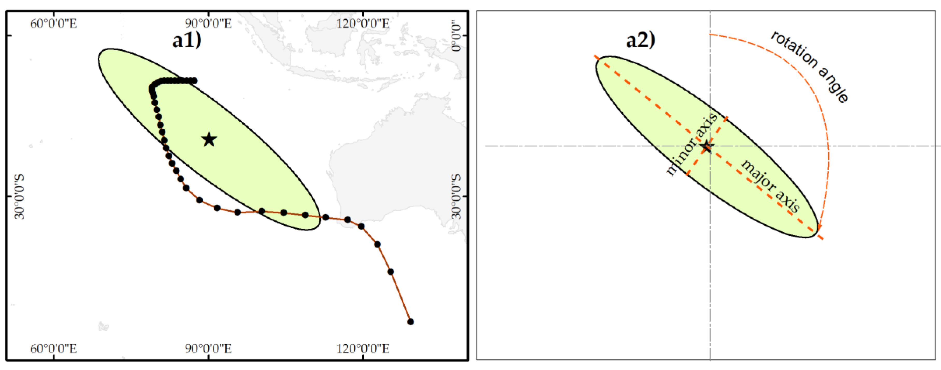
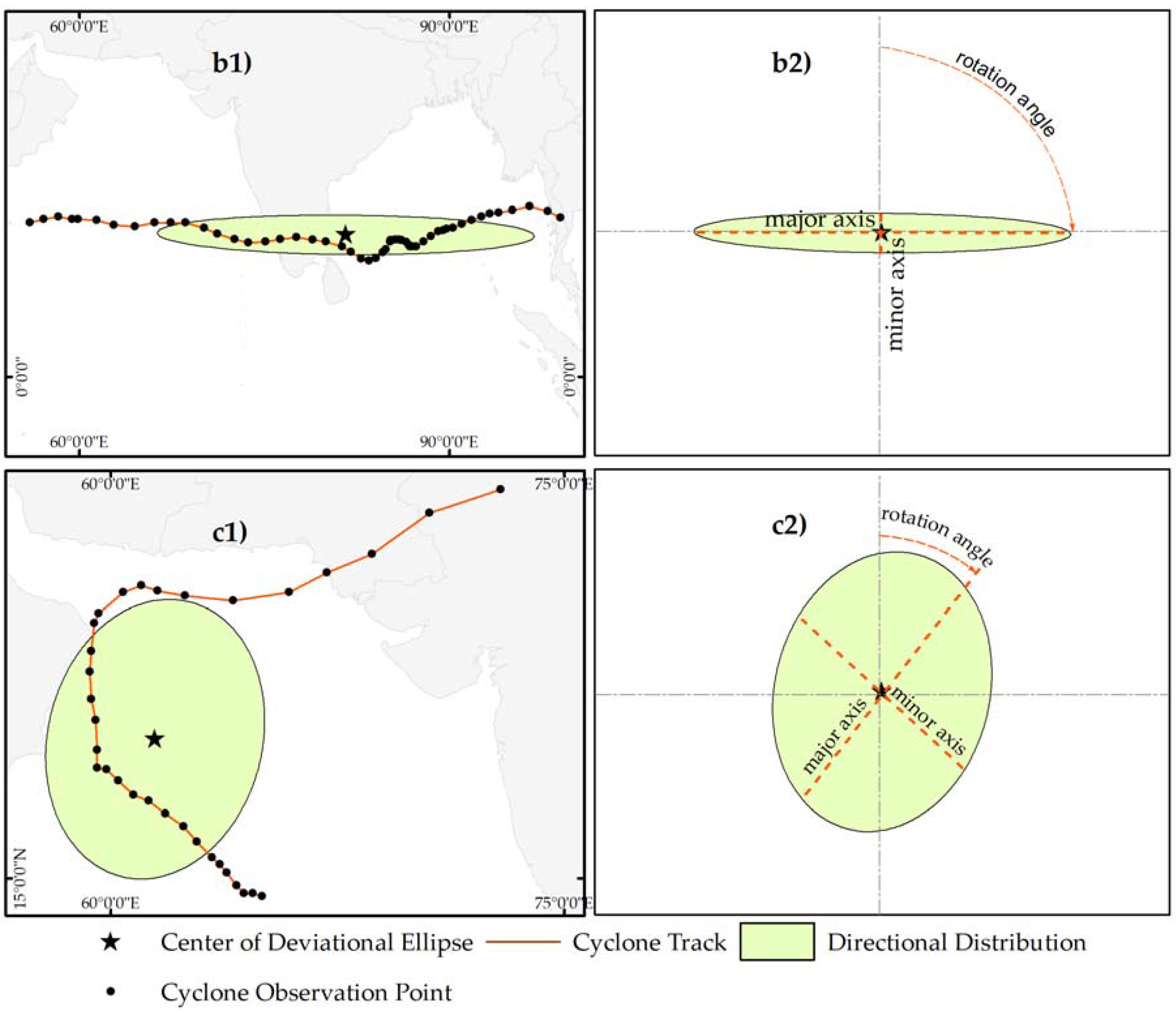
The left panels of Figure 1 show examples of the standard deviational ellipse of three cyclone tracks. The weighted mean center is the centroid of the observations which may fall on or off the cyclone track (Figure 1a–c). The rotation angle of the ellipse is the clockwise angular measure from the north to the long axis of the ellipse. This angular measurement is always between 0° to 180° because the long axis can always be found on the right side of the vertical axis. The right panels of Figure 1 illustrate the five parameters: center coordinates, two axes, and the rotation angle of the corresponding standard deviational ellipse. Many turns in the cyclone track may lead to a near-circular ellipse (Figure 1c). These five parameters are equivalent to the mean center, variances, and covariance [52]. The detailed mathematical expressions are given in Equations (1)–(7) in the methodology section. The latter group of five track parameters are used for clustering TCs based on the K-means algorithm. Each of the clusters is then assessed based on intensity, genesis location, landfall, total cyclone accumulated energy, seasonality, and trend.
Clustering analysis is generally an unsupervised approach to find the similarities among the data points and to group them. There are many clustering methods available, such as K-means clustering [53], probabilistic Curve-aligned clustering and prediction with regression mixture models [54], fuzzy clustering [55], and so on. The K-means clustering is one of the most popular clustering techniques for its simplicity and is used for clustering cyclones in different basins [4,56,57,58]. The K-means algorithm divides N points in D dimensions into k clusters, where the summation of the variance within a cluster is minimized to ensure the objects of each cluster are as close to each other as possible [59]. The feature space and the number of clusters are two important considerations in the K-mean clustering algorithm. In this analysis a five-dimensional feature space is used for the clustering with the Euclidian distance metric; since the K-means clustering algorithm uses a distance function to find the dissimilarity, one possible issue may be that the five elements have different scales in measurement and, therefore, need to be normalized so that five elements have the same weight to the clustering process. Therefore, these elements are normalized to the scale between 0 to 1 by max-min normalization ((x−min)/(max−min)).
The second important aspect is to set the number of clusters since the result completely depends on the initial setting of the cluster number. Although it is difficult to determine the global optimal number of clusters, there are several ways to select a reasonable k-number. In this study, the number of clusters is determined by the mean silhouette values and numbers of negative silhouette values. Rousseeuw [60] stated that the silhouette is both the measurement of cohesiveness and separability of the clusters. The silhouette value for each observation is a measure of how similar these observations within the same cluster are when compared to the observations in other clusters. The silhouette of the ith observation (Si) can be defined by the normalized differences between the average distance from the ith observation to the other observations in the same cluster and the minimum average distance from the ith observation to observations in different clusters. The silhouette value for the ith point, Si, can be expressed by the following equation:
where ai is the average distance from the ith observation to the other observations in the same cluster, and bi is the average distance from the ith point to points in a different cluster [60]. The minimum is taken across all other clusters.
The valid silhouette values are in between −1 and 1. The mean silhouette value expresses the cohesiveness of the clusters, whereas the number of negative silhouettes refers to possible misclassification. Therefore, an optimum number of clusters should be chosen in such a way where the mean silhouette is high, and the number of the negative silhouettes is low. In this study, the K-means cluster algorithm was run multiple times for 2 to 20 clusters, and the mean silhouette value and the negative silhouette counts were calculated for each run. Figure 2 shows the plot of the mean silhouette and the corresponding number of negative silhouette counts with different cluster numbers. The highest mean silhouette and the lowest number of negative silhouettes take place when the cluster number is four. Therefore, the number 4 is the optimal number of clusters for the current study based on the silhouette criterion.
2.3. Analysis of Large-Scale Climate Variabilities
The SST anomaly composite is constructed by taking the mean of weekly SSTA prior to the TC genesis in each cluster. The long-term mean of daily OLR is subtracted from the daily OLR to obtain the daily OLR anomaly. The mean of the daily OLR anomaly two days prior to the cyclone genesis is calculated to obtain the daily composite of the OLR anomaly for each cluster. The reason to take the climatic conditions prior to the cyclone genesis is to avoid possible contamination of environmental conditions by the TC circulation itself [16]. Descriptive statistics are calculated on the SST and the OLR for TCs in each cluster. Kernel density estimation (KDEs), a non-parametric technique for continuous density estimation [61] of TC genesis, is also calculated to visualize the spatial association between genesis location and large-scale climate variabilities.
2.4. Statistical Significance Test
It is important to determine whether clusters are significantly different from each other. The Kruskal–Wallis test, a nonparametric test, is suitable for the current study because there are more than two samples. This significant test examines if there is a significant difference in the central tendency of samples based on the ranked observation [62]. Since the current study has four clusters, the statistical significance among clusters can be tested for different valuables. While the Kruskal–Wallis test is suitable to see the overall difference among clusters, the multiple paired Mann–Whitney U test can compare the differences between two clusters. Therefore, to find the similarities and dissimilarities between clusters the Mann–Whitney U test is applied for all the variables. Significance of the trend is tested based on the t-test at the 95% confidence level.
3. Results and Discussion
3.1. Genesis Location and Track Shape
The genesis is the first observed location of a cyclone. Figure 3 shows TC genesis location in each cluster. TCs in the SIO are formed mostly between 5° S and 25° S where the TC heat potential is high, which is a favorable condition for cyclone intensification [19]. The genesis ranges of three clusters in the SIO are overlapped (Table 1). The mean genesis location of Cluster 1 is at 115° E and 11.4° S, indicating the majority of the cyclones in this cluster are formed near the northeast side of the SIO. The cyclones in Cluster 1 make a parabolic turn towards the Australian coast (Figure 3). The mean genesis of Cluster 2 is at 78.3° E and 10.5° S, and the mean genesis of Cluster 3 is at 64.7° E and 12.5° S. The mean genesis locations of Cluster 2 and Cluster 3 indicate that the cyclones of these two clusters are formed mostly in the middle of the SIO. The locations of these three clusters are very similar with the three broad clusters of Ash and Matyas [63], where they applied second-stage clustering on the start and end of TC tracks. Many cyclones from Cluster 2 and Cluster 3 did not make landfall because the whole lifespan of these cyclones passed over the deep ocean. Only a few of the cyclones in Cluster 2 move towards the African coast (Figure 3). In general, cyclones in Cluster 3 move toward the African coast, but some of them make a parabolic turn near Madagascar and move away from the coast. Only a few cyclones in Cluster 2 are formed near the Indonesian coast, but they move towards the deep ocean. In contrast to other clusters, Cluster 4 has a narrow genesis longitude range (Table 1), but most of the cyclones in this cluster move in the northwest direction towards the Indian coast (Figure 3). Although most of the cyclones in the IO move in a westerly direction, few tracks of Cluster 4 move northeast to make landfall on Myanmar and India from the Bay of Bengal and the Arab Sea, respectively.
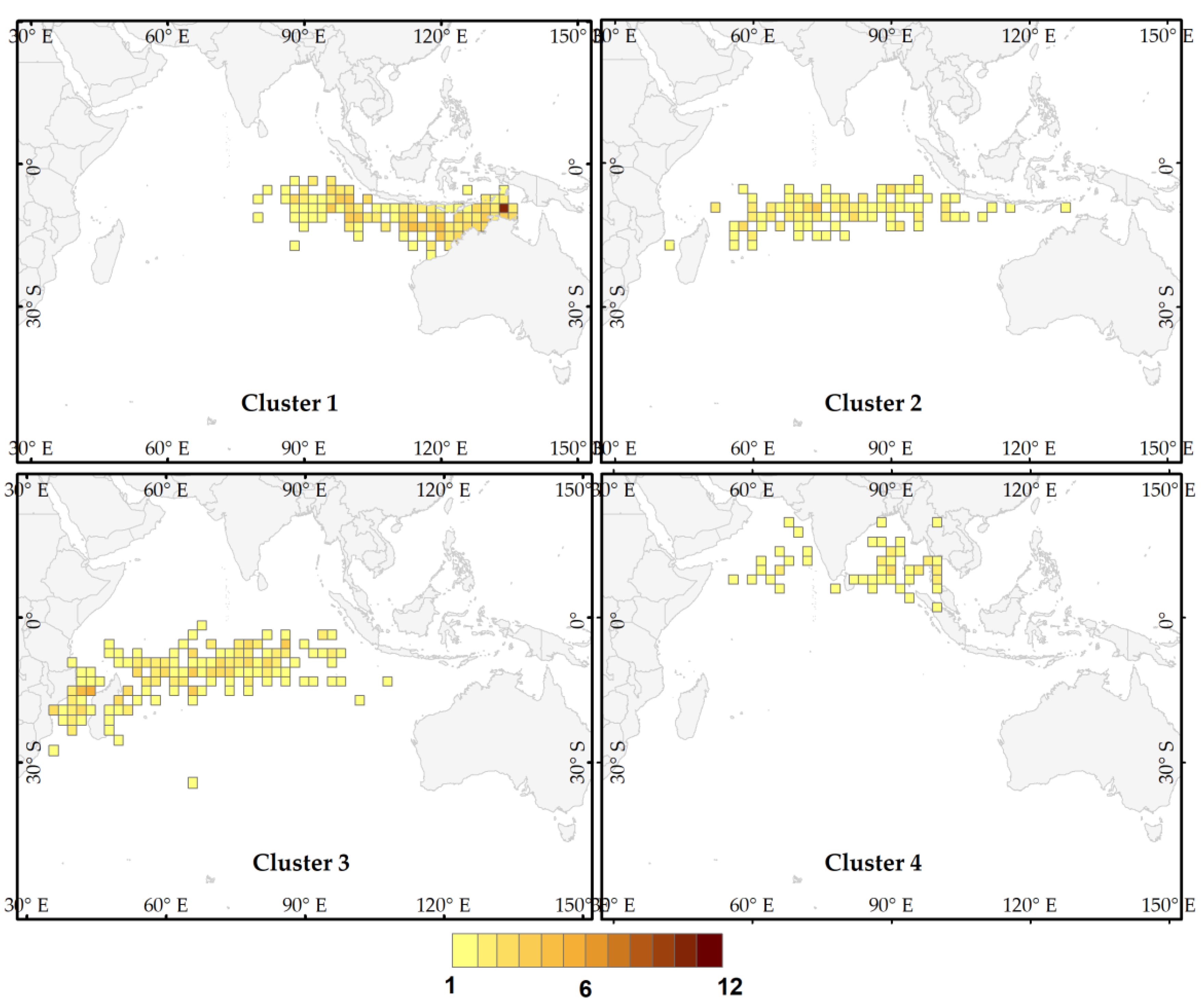
The extent of the Indian Ocean is divided into 2° by 2° grids to calculate the cumulative density of the cyclone genesis in each grid cell. The cumulative density of cyclone genesis is the total genesis counts in each grid. Figure 4 shows the cumulative density of cyclone genesis in each cluster. The very high density, 12 cyclones in a 2° grid cell, of Cluster 1 is found near the northern coast of Australia, between Australia and Indonesia (Figure 4). Genesis locations are diffused in Cluster 2, as none of the grid cells of this cluster has a very high cumulative density. Most of the grid cells in Cluster 3 have a moderate cumulative density of cyclone genesis location. Most of the grid cells in Cluster 4 show a very low genesis density.
3.2. Cluster Centroids and Properties
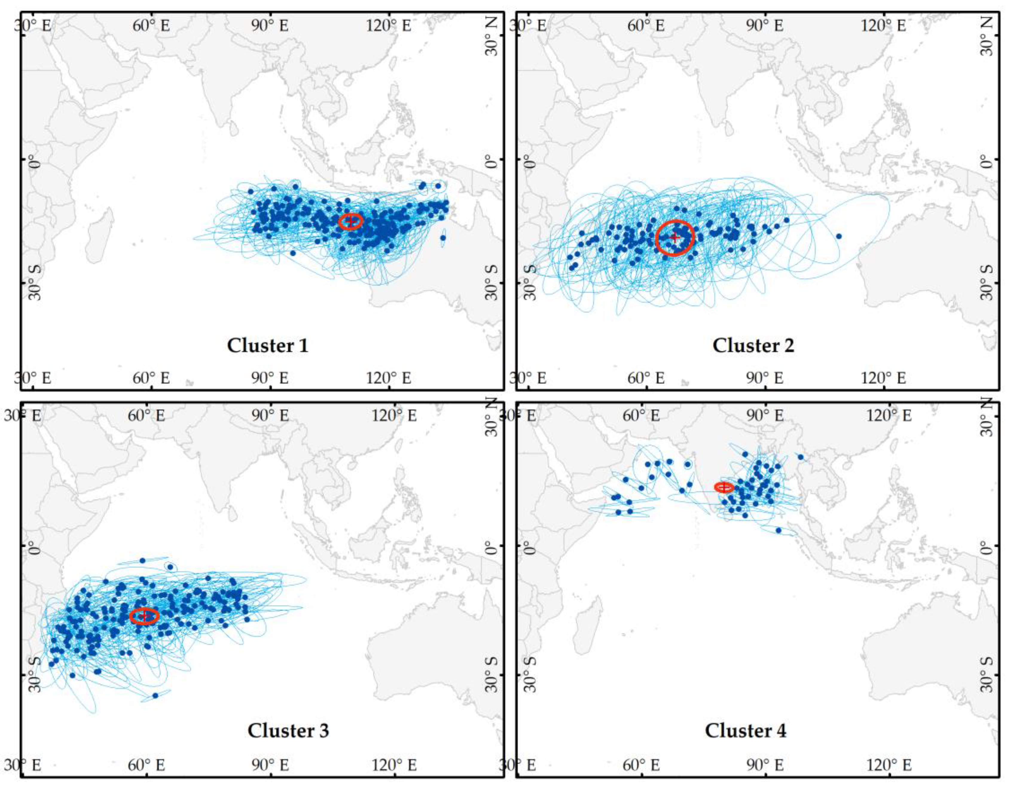
The standard deviational ellipses of all cyclones are grouped into four groups based on K-means clustering. Table 2 and Figure 5 show the basic mean properties of standard deviational ellipses in the four groups. From Figure 5, Cluster 1 is located on the northwestern side of Australia centered at 110° E and 16° S and the variance in the x-axis is more than double of the variance in y-axis. The mean centers of Cluster 2, located in the middle of the IO. Cluster 3 is located near the African coast, more specifically near Madagascar. The variance in the x-axis is almost three times of the variance in the y-axis in Cluster 3. The shape of the mean ellipse of Cluster 3 is elongated, whereas the shape of the mean ellipse is near-circular for Cluster 2. Cluster 4 is found in the Northern Indian Ocean (the Bay of Bengal and Arab Sea). This is the only cluster located in the Northern Hemisphere, whereas the other three clusters are in the Southern Hemisphere. The mean center of Cluster 4 is located near the Indian coast at 80° E and 14° N.
3.3. Cyclone Intensity, Track Length, Rotation, and Lifespan
The deviational ellipse of a cyclone is directly affected by the wind speed, track length, and lifespan of the cyclone. Long lifespan causes large deviational ellipse unless the tropical cyclone is slow moving. The major and minor axes of the ellipse depend on the curve of the track. A long track with little turning may result in a long major axis and a track with many turns results in a relatively long minor axis. Figure 6, Figure 7, Figure 8, Figure 9 and Figure 10 illustrate the distributions of cyclone intensity in knots, lifespan in days, track length in km, track rotation angle in degrees, and total accumulated cyclone energy (ACE) in knots2 in each cluster and all cyclones, respectively. The subsequent discussion of this article uses boxplots to explain different metrics related to cyclone. These boxplots are generated in the MATLAB (Natick, MA, USA) environment where extreme values in the data distribution are considered as outliers. According to the MATLAB definition, outliers are defined as the value outside of the range of ±2.7σ (approximately 99.3% coverage) [64].
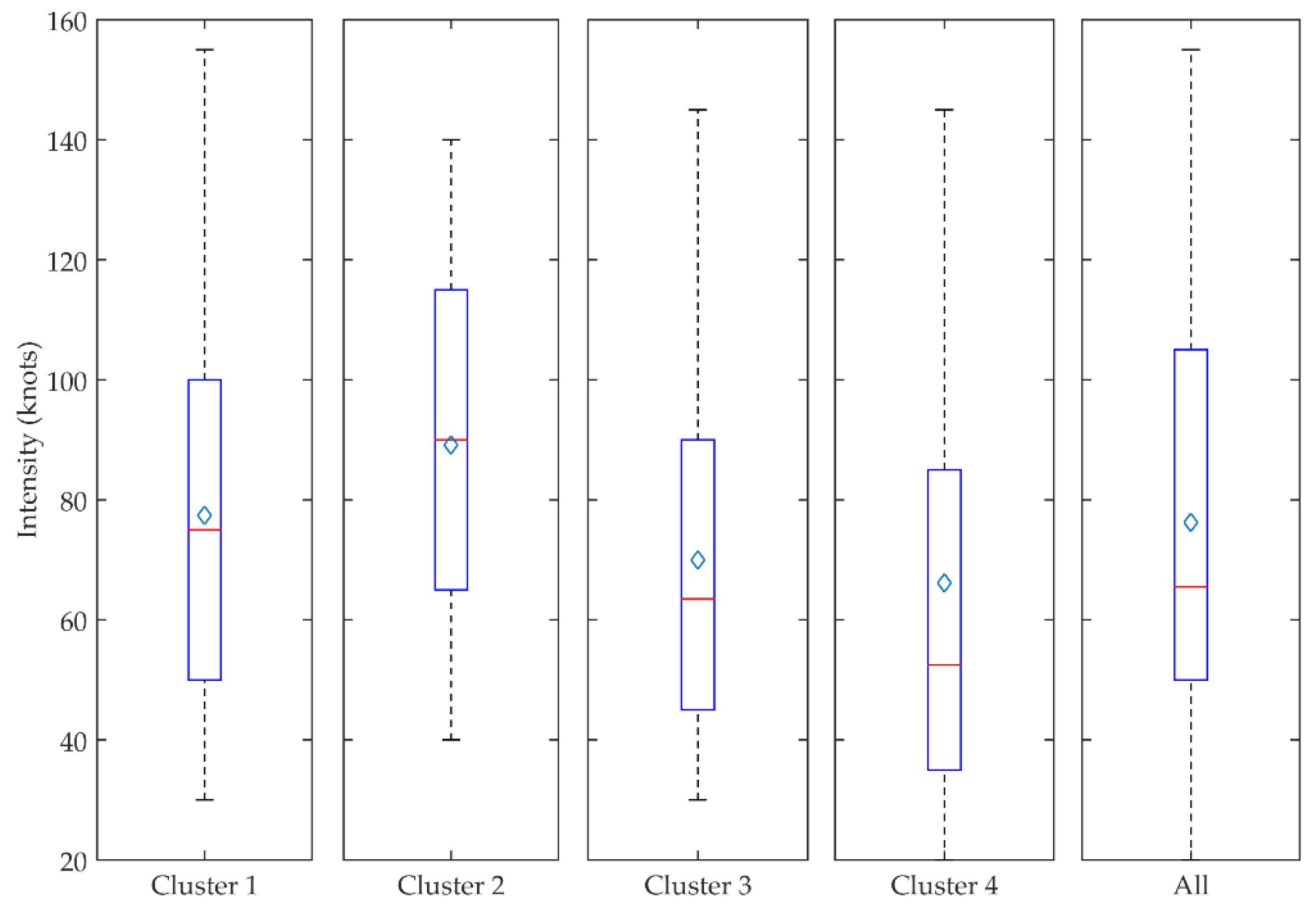
The maximum cyclone intensity is the maximum sustained wind during the entire life of a TC. The maximum intensity of cyclones in each cluster is shown in Figure 6. Different agencies are responsible for cyclone records in the sub-basins of the IO. These agencies use different intensity classes at different wind speeds. Therefore, the current study uses only one general scale, the Saffir-Simson scale, for the common understanding of intensity discussion. The Saffir-Simpson scale categorizes cyclones based on maximum wind speed, and the scale is as follows: Tropical Depression (TD) < 33 kt; Tropical Storm (TS) 33–63 kt; Category 1, 64–82 kt; Category 2, 83–95 kt; Category 3, 96–112 kt; Category 4, 113–136 kt; Category 5, >136 kt. Figure 6 shows that the cyclones in Cluster 2 are relatively stronger than other clusters. The intensity ranges of clusters vary significantly. The mean maximum intensity of Cluster 2 is higher than the mean intensity of the other three clusters. Cluster 3 and Cluster 4 have close interquartile ranges and the mean values of cyclone intensities. However, the median cyclone intensity of Cluster 4 is the lowest among the median intensities of other clusters. Cluster 1 and Cluster 2 have higher mean and median maximum intensities than the overall mean and median maximum intensity, whereas cluster 3 and Cluster 4 have lower mean and median intensities. The mean cyclone category of Cluster 2 is equivalent to Category 2, whereas, the mean cyclone category is equivalent to Category 1 in the other three clusters. The median category of Cluster 4 and Cluster 3 is TS. The distribution of the cyclone intensity of all clusters is right skewed, except Cluster 2, meaning that the mean value of cyclone intensities is higher than the median value. The skewness of the intensity distribution indicates most of the cyclones are in a lower category (Category 1 or TS).
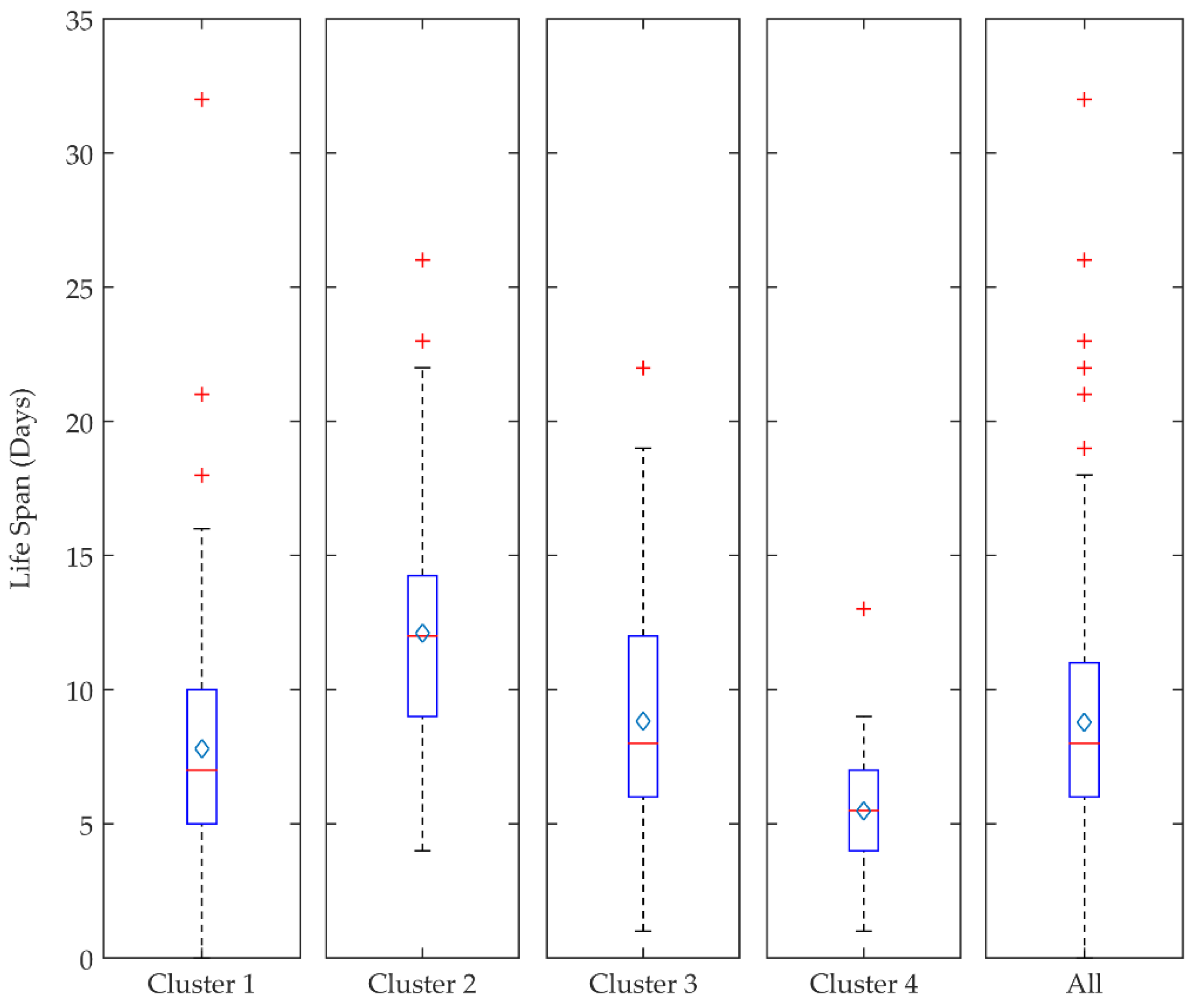
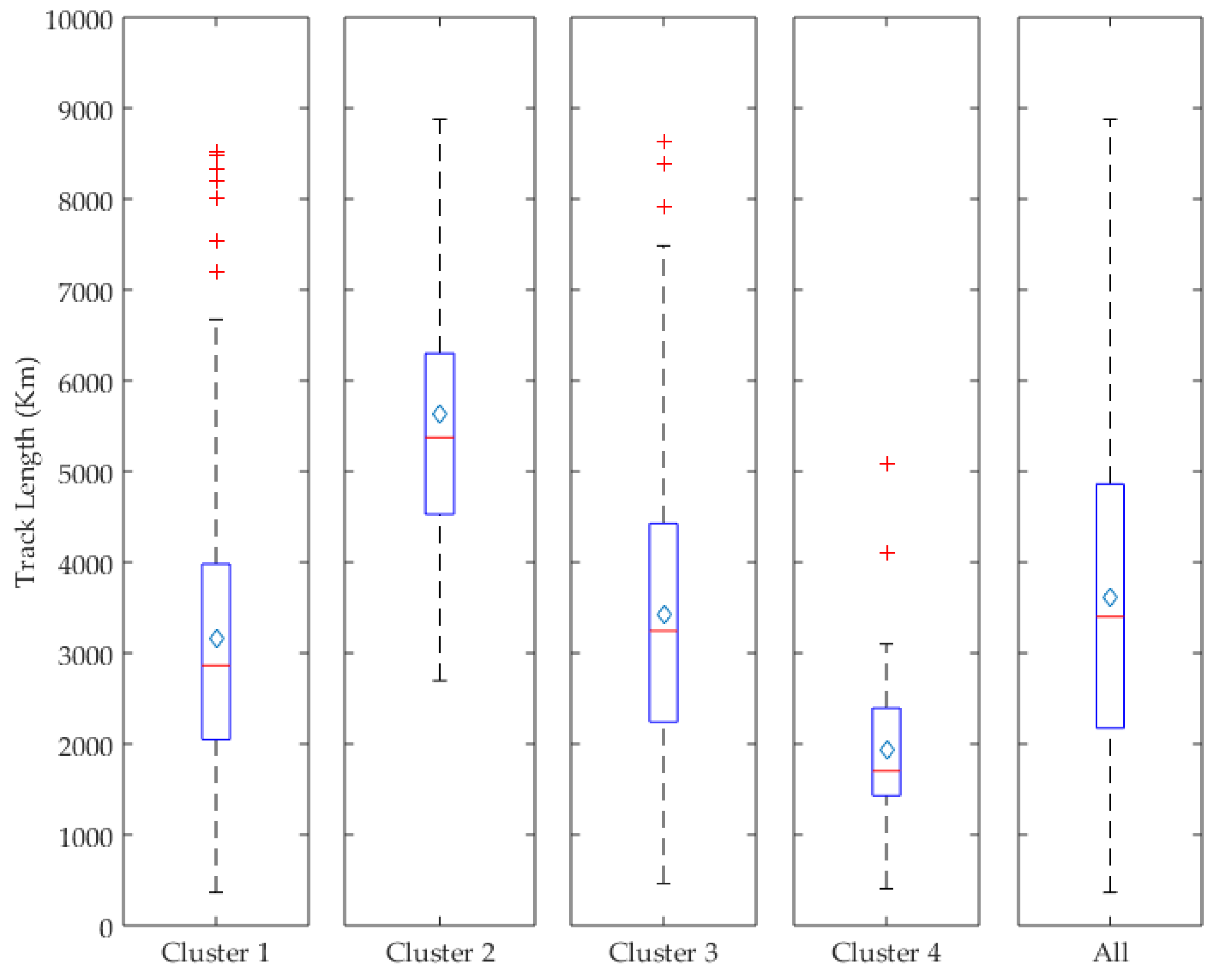
Figure 7 shows the lifespan of cyclones in each cluster in days. The mean lifespan and median lifespan of cyclones are highest in Cluster 2 and lowest in Cluster 4. Cyclones in the NIO are short-lived. The inter quartile ranges of clusters are very different. The interquartile ranges of cyclone lifespan in the three clusters the SIO are longer compared to Cluster 4 in the NIO. The mean lifespan is the smallest in Cluster 4 compared to other clusters (Figure 8). The mean and median lifespans of the cyclones in Cluster 4 are almost the same. The distributions of cyclone lifespan in all clusters are right-skewed, except Cluster 4. This right skewness indicates that most cyclones have a short lifespan than the average lifespan. The similar pattern can be found between lifespan and tack length for most of the clusters (Figure 7 and Figure 8). The size of the deviational ellipse depends not only on track length, but also on the turning of the cyclone path.
Figure 9 illustrates the distribution of the rotation angle of the standard deviational ellipse in each cluster. A clear separation can be seen in the percentile ranges of the rotation angle in Cluster 2 from the other clusters. The mean rotation angle of Cluster 2 is less than 70°, whereas the mean rotation angle of other clusters is above 80°. Cluster 4 has the highest mean rotation angle (more than 95°) among the clusters. Cluster 1 has the largest percentile ranges of cyclone rotation angles, which means a large variation of the cyclone path direction exists in this cluster. Interestingly, the distribution of the rotation angle is right skewed for clusters in the SIO, however, the distribution is left skewed for cyclones in the NIO.
The total accumulated cyclone energy (ACE) is a wind energy index used by the National Oceanic and Atmospheric Administration (NOAA), which is defined as the sum of the squares of the maximum sustained surface wind estimates at 6-h intervals [65]. This is a widely-used index for cyclone intensity analysis. The ACE distributions displayed in Figure 10 show that Cluster 1 and Cluster 3 have very similar distributions. The percentile ranges of Cluster 2 is higher than other clusters. The mean ACE is the highest and the lowest in Cluster 2 and in Cluster 4, respectively. There are a number of outliers in the distribution, indicating unusual ACE resulted from higher category long-lived cyclones. From lifespan (Figure 7), track length (Figure 8), and ACE (Figure 10), it can be observed that the longest mean lifespan, the longest mean track length, and the highest energy accumulation are found in Cluster 2 and the lowest in Cluster 4 because longer lifespan results in higher energy accumulation. The distributions of ACE are positively skewed in all clusters, indicating the majority of the cyclones are less intense than the mean ACE of cyclones.
3.4. Seasonality
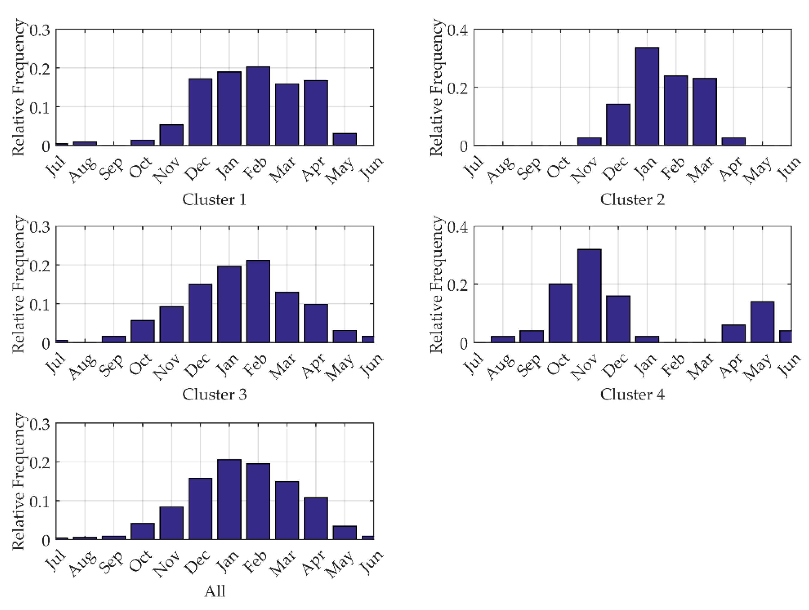
Figure 11 shows an interesting variation in cyclone relative seasonality in the IO. The longest season can be observed in Cluster 3 from August through June. Cluster 2 has seasonality similar to Cluster 3, mainly from December to April. Though there are variations in the cyclone season, the monthly distribution of Clusters 1, 2, and 3 indicate that most of the cyclones in these three clusters are in December to March. Since these three clusters are in the SIO, cyclones of these clusters have a similar season, which is completely different from Cluster 4 in the NIO. Figure 11 shows two different seasons of the NIO: pre-monsoon and post-monsoon. The pre-monsoon season is short (April–May) compared to the post-monsoon season (October–December). The reason behind two seasonal peaks is the Indian monsoon, when the southeast wind from NIO moves toward land. Upper-level winds from the NIO are too brisk (strong vertical wind shear) during the monsoon to form a cyclone in the additional unusual season (April–June). Singh et al. [66] described that cyclones in the pre-monsoon season in this area (Cluster 4) usually moved northward and cross the northwestern coast of India and the coast of Bangladesh. On the other hand, most of the post-monsoon cyclones hit the southeastern coast of India and the coast of Sri Lanka. Figure 12 illustrates the distribution of cyclone month in each cluster. Clusters in the SIO have similar interquartile ranges. January is the median cyclone month of Cluster 2 and Cluster 3, as well as February is of Cluster 1. Cluster 3 has the longest season, nearly ten months of the year, compared to other clusters in the SIO, whereas Cluster 2 has the shortest season among the clusters. In contrast to these three clusters, Cluster 4 has most of the cyclones in November and Cluster 4 has the longest seasonality among clusters considering the two cyclone seasons in the NIO. The distribution of the cyclone month is skewed because of the additional season in the summer.
3.5. Landfall
Landfall of a cyclone is important in the context of disaster risk. The risk is the function of the hazard (cyclone) scale and the vulnerability of the community [61]. From the disaster risk paradigm, there is higher risk associated with cyclones that make landfall than the cyclones that do not make landfall. For instance, a cyclone with high intensity and high accumulated energy which formed and ended over in the deep ocean, may not be as harmful as a low-intensity landfall cyclone. Landfall is considered as an event when a storm moves over the land surface. The intensity at the time of landfall is considered as the landfall intensity of the cyclone. Table 3 shows the landfall frequency and percentage of each cluster and Figure 13 shows the landfall locations of cyclones. Although Cluster 4 accounts for only 8.6% of total cyclones, it has the highest percentage (84.31%) of landfall. In contrast, more than one-third of Indian Ocean cyclones are in Cluster 1, only half of these cyclones made landfall. Both Clusters 2 and 3 together comprise half of the Indian Ocean cyclones, but the percentage of landfall is low compared to Clusters 1 and 4.
Table 3 shows that 14.3%, 35.9%, 27.47%, and 13.9% of landfall cyclones are higher category (1–4) cyclones at the time of landfall in Clusters 1, 2, 3, and 4, respectively. Though Cluster 1 has a higher number of cyclones, the percentage of high-intensity cyclones is low compared to other clusters located in the SIO. Most of the cyclones in Cluster 1 made landfall at the Australian and Indonesian coast, and only a few of them are very strong cyclones (Category 1–4). The majority of cyclones in both Cluster 2 and Cluster 3 made landfall at the coast of the East Africa, more specifically on the coast of Madagascar and Mauritius. Although, the TCs in cluster 3 have higher percentage than those in cluster 2 to make landfalls, Cluster 2 has the highest percentage of strong cyclones among all clusters. Cluster 2 has the highest mean accumulated cyclone energy (Figure 10), but the lowest percentage of landfall cyclones. This is because the tracks in cluster 3 have less curvature than those in Cluster 2, as shown by the mean ellipse shapes in Figure 5. Most of the cyclones of Cluster 4 struck the coast of the Bay of Bengal and some of them made landfall on the coast of the Arabian Sea.
3.6. Trend Analysis
Trend analysis is very important because it gives a general idea of how the number of cyclones increase or decrease over the years. Many researchers have tried to describe the trend of cyclones in different ocean basins for both cyclone numbers and intensity [33,66,67]. To determine the trend, the number of cyclones and the total accumulated cyclone energy are plotted against years in Figure 14 and Figure 15, respectively. Two trend lines are added to each plot using a simple Savitzky-Golay filter and linear regression. p-values for linear regression, 0.5669, 0.8545, 0.3474, and 0.0000, for Clusters 1–4, respectively, indicate that while the cyclone frequency trend is not significant in the SIO, it is in the NIO. The simple linear regression curve shows the overall trend (red lines), while the trend line results from the Savitzky-Golay filter show the local trend of inter-year variation (green lines). Figure 14 demonstrates a decreasing trend in number of cyclones per year in Clusters 1 and 3. Only Cluster 4 shows a rapid TC number increase in the last 15 years. Supporting this, Webster et al. [67], show that the SST of the NIO increased in recent time. They also found that SST is one of the most important influences on the cyclone occurrence. The total number of cyclones increases in the NIO because cyclone frequency increases in the pre-monsoon month of May and the post-monsoon month of November [66]. Considering the interdecadal variations, cyclone frequency of cluster 2 was dropped in the mid-1990s; however, Cluster 3 had an increasing trend in the mid-1990s (Figure 14). Cyclone frequency in Cluster 1 follows an almost steady trend from 1981 to 2015.
Total accumulated cyclone energy is directly related to cyclone lifespan and intensity. Thus, the trend of cyclone energy accumulation may be related to the number of cyclones. However, the total energy of many short-lived weak cyclones may not be as high as a small number of strong long-lived cyclones. As shown in Figure 15, the total accumulated energy increases in Cluster 3 and Cluster 4. In contrast, Clusters 1 and 2 follow a decreasing trend in total accumulated energy. Only the trend of Cluster 4 is significant at the 95% confidence level, p-values of t-statistics are 0.1099, 0.5930, 0.9451, and 0.0001 for Clusters 1 to 4, respectively. Similar to the number of cyclones per year, the trend of total accumulated energy is following a linear rise in Cluster 4. This result is supported by the finding of Singh et al. [66], who claimed that severe cyclones (cyclone with high energy) in the NIO doubled in number in recent decades. Among the clusters in the SIO, ACE decreased in Cluster 2, but increased in Clusters 1 and 3 in the 1990s. Although the cyclone frequency trend was almost steady in Cluster 1, the total accumulated energy increased in the mid-1990s, followed by a gradual decreasing trend. The ACE per year in Cluster 3 follows a declining trend in the mid-1980s and returns to the previous level in the 1990s. The trend of overall yearly ACE in the Indian Ocean follows a gradual increment over the 1980s and 1990s followed by a decrease trend until 2002, then starts a linear rise again. The trend of cyclone frequency and accumulated energy per year varied over the period from 1981 to 2015. The important fact is that the cyclones with the hazardous potential increases in number in Cluster 4. Therefore, the disaster risk increases at the coast of the NIO due to the high percentage of landfall cyclones, as demonstrated by the increasing cyclone trend in Cluster 4.
3.7. Large-Scale Environmental Variabilities and TC Genesis
The variation of the summary statistics of the TC behaviors and temporal trends in the different clusters are associated with TC impacting physical parameters, such as SST and OLR. The composite of OLR anomalies two days prior to TC genesis in each cluster shows the strong relationship of TC genesis location and negative OLR anomalies (Figure 16). Genesis density in each cluster is co-located with the negative anomalies in OLR, which support the observation from previous studies that the negative OLR anomaly is one of the precursors for cyclone formation [20,31]. OLR anomalies are mostly between −5 Wm−2 and −15 Wm−2. Higher negative OLR anomalies, above −15 Wm−2, are found in Cluster 2, which is located between 0° S and 10° S in the SIO (Figure 16). Both Cluster 1 and Cluster 4 have two OLR anomaly zones. Two zones in Cluster 4 are associated with the Bay of Bengal and the Arab Sea. One zone in Cluster 1 is located near the Australian coast and another one is in the west side of Indonesia. Ramsay et al. [16] found two separate concentrations in these two zones in Cluster 1. Figure 17 shows the descriptive statistics of daily OLR two days prior at the location of TC genesis. Similar interquartile ranges of OLR are found in both Cluster 2 and Cluster 3, roughly between 160 Wm−2 and 225 Wm−2, with a mean OLR around 190 Wm−2. Although interquartile ranges of OLR in Cluster 3 are nearly similar to Cluster 1 and Cluster 2, a median value of 179 Wm−2 indicts that most of the TCs in Cluster 1 are formed at lower OLR. On the other hand, Cluster 4 has a lower interquartile range of OLR, roughly between 130 Wm−2 and 200 Wm−2, which indicates TCs are formed in the lower OLR in the NIO as compared to the SIO.
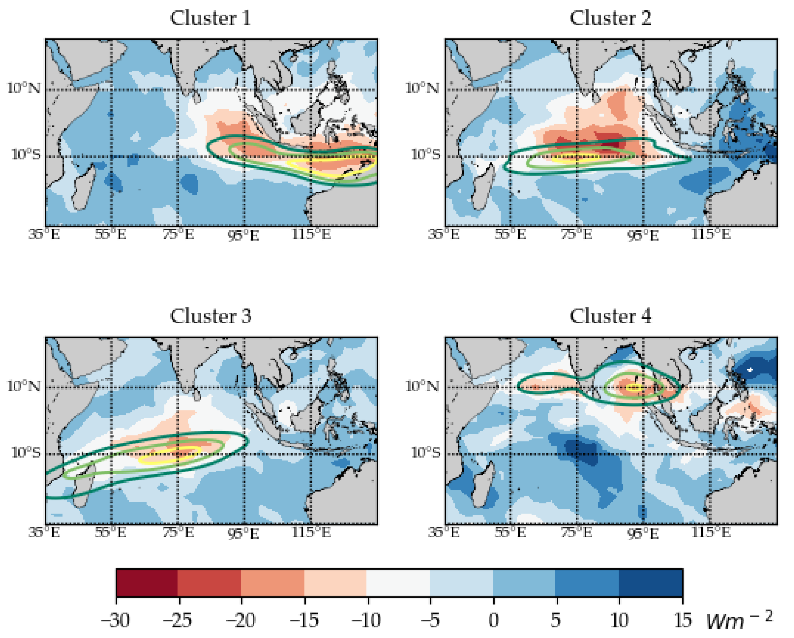
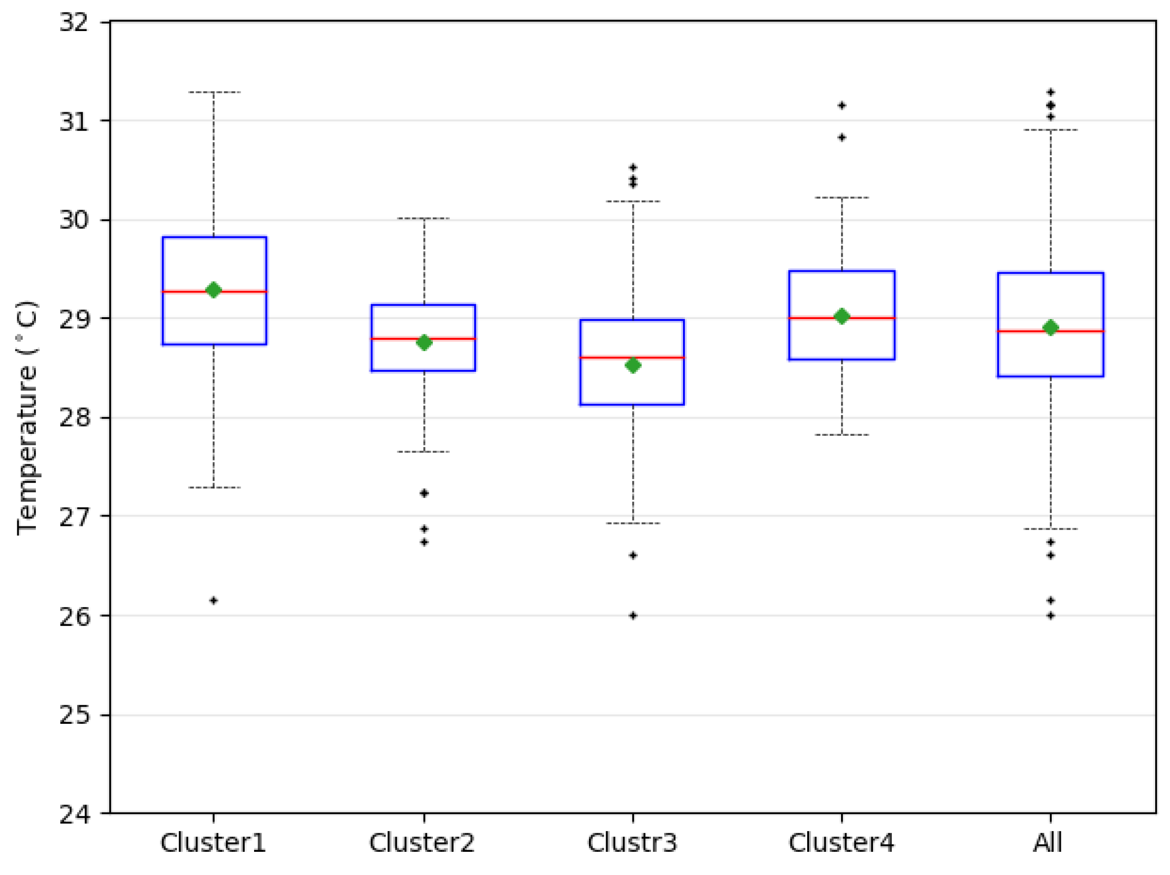
Figure 18 illustrates the composite weekly SST anomaly (SSTA) prior to TC genesis and the kernel density of TC genesis in each cluster. TC genesis is co-located with the higher positive SST anomalies near the Australian coast. Although Cluster 2 has two positive SSTA zones, TC genesis is mostly co-located at the middle SIO. Cluster 3 is associated with very low positive SSTA in the WSIO, indicating that TCs can form at low SSTA compared with other clusters. It is interesting to note here that very high positive weekly SSTA are found all over the IO prior to the TC genesis in Cluster 4 in the NIO. Although Ramsay et al. [16] mentioned that SSTA signals are part of the larger warming signals across the Indo-Pacific region rather than being constrained to the TC formation zone, the current study found the local SSTA zone in all clusters, except Cluster 4. The descriptive statistics of weekly SST at the location of TC genesis of each cluster is shown in Figure 19. Interquartile ranges of the weekly SST are narrow, but mostly vary across clusters. This narrow range (<2 °C) indicates the very specific temperature condition for TC formation. Of the four clusters, Cluster 1 has highest mean SST and Cluster 3 has the lowest mean SST. The mean SST of three clusters in the SIO are high to low from Cluster 1 to Cluster 3, which indicates the favorable SST of TC formation is low to high from east to west of the SIO.
3.8. Statistical Significance of the Clusters
The differences among these four clusters across the seven variables of TC attributes and environmental conditions are analyzed using the Kruskal–Wallis statistical significance test and the Mann–Whitney U tests (Table 4 and Table 5). All variables, except OLR, are statistically significant at the 95% confidence level. Therefore, we can reject the null hypothesis that samples are from the same probability distribution. TCs in Cluster 2 are characterized by higher intensity, longer lifespan, and track length, as well as higher ACE, because of the ideal condition of TC intensification in the middle of the SIO. In contrast, Cluster 4 has the lowest median intensity, lifespan, track length, and energy accumulation compared to other clusters. Cluster 2 and Cluster 3 have lower SST, but higher OLR, at the TC genesis location compared to the other two clusters. Therefore, SST at genesis may not be a good indicator of overall energy potentials since these storms tend to move over a large region after formation.
Table 5 shows the similarities and dissimilarities between clusters based on the pairwise Mann–Whitney U significance test. Most of the pairwise comparisons show the significant difference between clusters at the 95% confidence level. There is no significant difference between Cluster 3 and Cluster 4 considering maximum cyclone intensity and rotation angle. Cluster 1 and Cluster 3 have similar cyclone month and energy accumulation. Among six comparisons only half show significant differences of OLR at the locations of cyclone genesis.
4. Conclusions
The research on cyclone patterns and characteristics is important and of interest to many scientists because tropical cyclones are one of the most destructive natural hazards. Tropical cyclones may potentially follow similar characteristics—landfall, intensity, energy accumulation—if their genesis and track characteristics are similar. This study clusters IO cyclones based on the standard deviational ellipse of cyclone trajectories using the K-means clustering algorithm. Clusters also explain other characteristics of the cyclones, such as intensity, landfall, trend, accumulated energy, and large scale environmental variabilities, SST, and OLR.
In summary, the current study finds four clusters, one in the NIO and three in the SIO, after examining 592 TC tracks over the IO between 1981 and 2015. There are 230, 116, 195, and 51 TC tracks grouped into Cluster 1, Cluster 2, Cluster 3, and Cluster 4, respectively. Long track length, higher intensity, and long lifespan lead to the higher accumulated energy in Cluster 2, which may be because of the location of this cluster in the middle of the SIO. The rotation angle with the common genesis patterns may also explain the landfall as most cyclones move westward. Therefore, with the general westward movement, a large rotation angle indicates the probable track movement towards the northwest, while a small rotation angle is the indication of southwest movement. To know the eastward movement of cyclones, cyclone genesis and the end location need to be analyzed in future research. The Australian coast experienced the landfall of TCs from Cluster 1. Although spatial zones of genesis locations in both Cluster 2 and Cluster 3 are overlapped (Figure 3 and Figure 5), Cluster 3 has a higher percentage (54%) of landfall cyclones with high intensity (Category 1–4) compared to Cluster 2 (34%). Some clusters may be diffused (Cluster 2) and some clusters may be relatively compact (Clusters 1 and 3). Though the genesis location of most of the cyclones in both Cluster 2 and Cluster 3 are overlapped, the mean rotation angle of these two clusters are different. The low median rotation angle of Cluster 3 indicates a southwest movement of most of the TC tracks in the cluster, whereas some of the cyclones in this cluster have a large rotation angle because of recurvation of the track. Cluster 4 in the NIO is unique compared to other clusters, for not only spatial location, but also for other characteristics, such as seasons (e.g., only Cluster 4 has two seasons). The cyclone frequency and total accumulated energy linearly increase over the last two decades in Cluster 4. Though the number of cyclones in Cluster 4 is fewer compared to other clusters, this cluster has a high percentage of landfall. Both cyclones with high ACE and a high percentage of landfall cyclones of Cluster 4 may have higher disaster risk potentials. Another interesting finding is that the intensity (Figure 6), lifespan (Figure 7), track length (Figure 8), and accumulated cyclone energy (Figure 10) follow a similar pattern in the comparison among clusters. This pattern indicates that longer track length, long lifespan, and higher intensity make for higher energy accumulation. The genesis locations are co-located with the negative OLR anomalies. Positive SSTA are co-located with the TC genesis in three clusters in the SIO. TC genesis in Cluster 1 is associated with high SSTA in the IO. SST anomalies are localized in three clusters over the SIO. TC genesis is associated with a very narrow band of SST, between 28 °C and 30 °C in all clusters.
The information on these clusters is helpful to understand the pattern of cyclones in different locations in the IO. Other meteorological conditions such as wind shear, and IOSD- and ENSO-related parameters of these four clusters need to be investigated. The relation of clusters with SST, OLR, and other meteorological factors can be linked to cluster characteristics in predicting the pattern and nature of future cyclones. These kinds of predictions will help to determine possible landfall of cyclones and to determine the potential risk for cyclones, which will be helpful for disaster risk reduction for cyclone-vulnerable societies around the Indian Ocean. Further research on tropical cyclones will be helpful for disaster risk reduction for cyclone-vulnerable societies around the Indian Ocean.
Author Contributions
R.Y. and L.D. conceived and designed the experiments; M.S.R. performed the experiments; M.S.R. and R.Y. analyzed the data; and all authors contributed to the writing of this paper.
Acknowledgments
This study was supported by grants from the NASA Applied Science Program (Grant #NNX14AP91G and #NNX15AK27A, PI: Liping Di). We would like to thank National Centers for Environmental Information (NCEI) for International Best Track Achieve for Climate Stewardship (IBTrACS) data. We are also thankful to NOAA for NOAA_OI_SST_V2 data and Interpolated OLR data provided by the NOAA/OAR/ESRL PSD, Boulder, CO, USA. Authors would also like to thank the anonymous reviewers for their valuable comments and suggestions.
Conflicts of Interest
The authors declare no conflict of interest.
References
- Mu, M.; Zhou, F.; Wang, H. A Method for Identifying the Sensitive Areas in Targeted Observations for Tropical Cyclone Prediction: Conditional Nonlinear Optimal Perturbation. Mon. Weather Rev. 2009, 137, 1623–1639. [Google Scholar] [CrossRef]
- Rahman, M.S.; Di, L. The state of the art of spaceborne remote sensing in flood management. Nat. Hazards 2017, 85, 1223–1248. [Google Scholar] [CrossRef]
- Rahman, M.S.; Ahmed, B.; Di, L. Landslide initiation and runout susceptibility modeling in the context of hill cutting and rapid urbanization: A combined approach of weights of evidence and spatial multi-criteria. J. Mt. Sci. 2017, 14, 1919–1937. [Google Scholar] [CrossRef]
- Nakamura, J.; Lall, U.; Kushnir, Y.; Camargo, S.J. Classifying North Atlantic Tropical Cyclone Tracks by Mass Moments. J. Clim. 2009, 22, 5481–5494. [Google Scholar] [CrossRef]
- Ahmed, B.; Kelman, I.; Fehr, H.K.; Saha, M. Community resilience to cyclone disasters in coastal Bangladesh. Sustainability 2016, 8, 805. [Google Scholar] [CrossRef]
- Hoque, M.A.-A.; Phinn, S.; Roelfsema, C.; Childs, I. Modelling tropical cyclone risks for present and future climate change scenarios using geospatial techniques. Int. J. Digit. Earth 2018, 11, 246–263. [Google Scholar] [CrossRef]
- Rahman, M.S.; Kausel, T. Coastal community resilience to Tsunami: A study on planning capacity and social capacity, Dichato, Chile. IOSR J. Humanit. Soc. Sci. 2013, 12, 55–63. [Google Scholar] [CrossRef]
- Paul, B.K. Why relatively fewer people died? The case of Bangladesh’s Cyclone Sidr. Nat. Hazards 2009, 50, 289–304. [Google Scholar] [CrossRef]
- Bangladesh, G. Cyclone Sidr in Bangladesh: Damage, Loss and Needs Assessment for Disaster Recovery and Reconstruction; Government of Bangladesh: Dhaka, Bangladesh, 2008.
- Fritz, H.M.; Blount, C.D.; Thwin, S.; Thu, M.K.; Chan, N. Cyclone Nargis storm surge in Myanmar. Nat. Geosci. 2009, 2, 448. [Google Scholar] [CrossRef]
- Webster, P.J. Myanmar’s deadly daffodil. Nat. Geosci. 2008, 1, 488. [Google Scholar] [CrossRef]
- Probst, P.; Proietti, C.; Annunziato, A.; Paris, S.; Wania, A. Tropical Cyclone ENAWO Post-Event Report; Joint Research Centre (JRC), The European Commission’s Science and Knowledge Service: Brussels, Belgium, 2017. [Google Scholar]
- Impact Forecasting. February 013 Global Catastrophe Recap; Aon Benfield: Chicago, IL, USA, 2013. [Google Scholar]
- Belanger, J.I.; Webster, P.J.; Curry, J.A.; Jelinek, M.T. Extended prediction of North Indian Ocean tropical cyclones. Weather Forecast. 2012, 27, 757–769. [Google Scholar] [CrossRef]
- Samson, G.; Masson, S.; Lengaigne, M.; Keerthi, M.G.; Vialard, J.; Pous, S.; Madec, G.; Jourdain, N.C.; Jullien, S.; Menkès, C. The NOW regional coupled model: Application to the tropical Indian Ocean climate and tropical cyclone activity. J. Adv. Model. Earth Syst. 2014, 6, 700–722. [Google Scholar] [CrossRef] [Green Version]
- Ramsay, H.A.; Camargo, S.J.; Kim, D. Cluster analysis of tropical cyclone tracks in the Southern Hemisphere. Clim. Dyn. 2012, 39, 897–917. [Google Scholar] [CrossRef]
- Frank, W.M. Tropical cyclone formation. In A Global View of Tropical Cyclones; University of Chicago Press: Chicago, IL, USA, 1987; pp. 53–90. [Google Scholar]
- Shay, L.K.; Goni, G.J.; Black, P.G. Effects of a warm oceanic feature on Hurricane Opal. Mon. Weather Rev. 2000, 128, 1366–1383. [Google Scholar] [CrossRef]
- Leipper, D.F.; Volgenau, D. Hurricane heat potential of the Gulf of Mexico. J. Phys. Oceanogr. 1972, 2, 218–224. [Google Scholar] [CrossRef]
- Gray, W.M.; Brody, L.R. Global View of the Origin of Tropical Disturbances and Storms; Colorado State University: Collins, CO, USA, 1967. [Google Scholar]
- Schade, L.R.; Emanuel, K.A. The ocean’s effect on the intensity of tropical cyclones: Results from a simple coupled atmosphere–ocean model. J. Atmos. Sci. 1999, 56, 642–651. [Google Scholar] [CrossRef]
- Matyas, C.J. Tropical cyclone formation and motion in the Mozambique Channel. Int. J. Climatol. 2015, 35, 375–390. [Google Scholar] [CrossRef]
- Malan, N.; Reason, C.J.C.; Loveday, B.R. Variability in tropical cyclone heat potential over the Southwest Indian Ocean. J. Geophys. Res. 2013, 118, 6734–6746. [Google Scholar] [CrossRef]
- Knapp, K.R.; Kruk, M.C.; Levinson, D.H.; Diamond, H.J.; Neumann, C.J. The International Best Track Archive for Climate Stewardship (IBTrACS): Unifying Tropical Cyclone Data. Bull. Am. Meteorol. Soc. 2010, 91, 363–376. [Google Scholar] [CrossRef]
- TCFAQ. E25) Which Countries Have Had The Most Tropical Cyclones Hits? Available online: http://www.aoml.noaa.gov/hrd/tcfaq/E25.html (accessed on 14 February 2018).
- Gray, W.M. Hurricanes: Their formation, structure and likely role in the tropical circulation. Meteorol. Trop. Oceans 1979, 77, 155–218. [Google Scholar]
- Rahman, M.S.; Kausel, T. Disaster as an Opportunity to Enhance Community Resilience: Lesson Learnt from Chilean Coast. J. Bangladesh Inst. Plan. ISSN 2012, 5, 1–11. [Google Scholar]
- Kossin, J.P.; Camargo, S.J.; Sitkowski, M. Climate modulation of North Atlantic hurricane tracks. J. Clim. 2010, 23, 3057–3076. [Google Scholar] [CrossRef]
- Colbert, A.J.; Soden, B.J. Climatological variations in North Atlantic tropical cyclone tracks. J. Clim. 2012, 25, 657–673. [Google Scholar] [CrossRef]
- Balaguru, K.; Taraphdar, S.; Leung, L.R.; Foltz, G.R. Increase in the intensity of postmonsoon Bay of Bengal tropical cyclones. Geophys. Res. Lett. 2014, 41, 3594–3601. [Google Scholar] [CrossRef]
- Camargo, S.J.; Wheeler, M.C.; Sobel, A.H. Diagnosis of the MJO modulation of tropical cyclogenesis using an empirical index. J. Atmos. Sci. 2009, 66, 3061–3074. [Google Scholar] [CrossRef]
- Jury, M.; Gadgil, S.; Meyers, G.; Ragoonaden, S.; Reason, C.; Sribimawati, T.; Tangang, F. Applications of An Indian Ocean Observing System to Climate Impacts and Resource Predictions in Surrounding Countries in the Context of ENSO-Monsoon Teleconnections; OceanDocs: Paris, France, 2000. [Google Scholar]
- Kuleshov, Y.; Qi, L.; Fawcett, R.; Jones, D. On tropical cyclone activity in the Southern Hemisphere: Trends and the ENSO connection. Geophys. Res. Lett. 2008, 35. [Google Scholar] [CrossRef]
- Liebmann, B.; Hendon, H.H.; Glick, J.D. The relationship between tropical cyclones of the western Pacific and Indian Oceans and the Madden-Julian oscillation. J. Meteorol. Soc. Jpn. 1994, 72, 401–412. [Google Scholar] [CrossRef]
- Jury, M.R.; Pathack, B. A study of climate and weather variability over the tropical southwest Indian Ocean. Meteorol. Atmos. Phys. 1991, 47, 37–48. [Google Scholar] [CrossRef]
- Suzuki, R.; Behera, S.K.; Iizuka, S.; Yamagata, T. Indian Ocean subtropical dipole simulated using a coupled general circulation model. J. Geophys. Res. 2004, 109. [Google Scholar] [CrossRef]
- Terry, J.P.; Gienko, G. Developing a new sinuosity index for cyclone tracks in the tropical South Pacific. Nat. Hazards 2011, 59, 1161–1174. [Google Scholar] [CrossRef]
- Terry, J.P.; Kim, I.-H.; Jolivet, S. Sinuosity of tropical cyclone tracks in the South West Indian Ocean: Spatio-temporal patterns and relationships with fundamental storm attributes. Appl. Geogr. 2013, 45, 29–40. [Google Scholar] [CrossRef]
- Leroy, A.; Wheeler, M.C. Statistical prediction of weekly tropical cyclone activity in the Southern Hemisphere. Mon. Weather Rev. 2008, 136, 3637–3654. [Google Scholar] [CrossRef]
- Nakamura, J.; Lall, U.; Kushnir, Y.; Rajagopalan, B. HITS: Hurricane intensity and track simulator with North Atlantic Ocean applications for risk assessment. J. Appl. Meteorol. Climatol. 2015, 54, 1620–1636. [Google Scholar] [CrossRef]
- Camargo, S.J.; Robertson, A.W.; Gaffney, S.J.; Smyth, P.; Ghil, M. Cluster Analysis of Typhoon Tracks. Part I: General Properties. J. Clim. 2007, 20, 3635–3653. [Google Scholar] [CrossRef]
- Villarini, G.; Vecchi, G.A.; Smith, J.A. US landfalling and North Atlantic hurricanes: Statistical modeling of their frequencies and ratios. Mon. Weather Rev. 2012, 140, 44–65. [Google Scholar] [CrossRef]
- McCloskey, T.A.; Bianchette, T.A.; Liu, K.-B. Track patterns of landfalling and coastal tropical cyclones in the Atlantic basin, their relationship with the North Atlantic Oscillation (NAO), and the potential effect of global warming. Am. J. Clim. Chang. 2013, 2, 12. [Google Scholar] [CrossRef]
- Ho, C.-H.; Kim, J.-H.; Kim, H.-S.; Choi, W.; Lee, M.-H.; Yoo, H.-D.; Kim, T.-R.; Park, S. Technical note on a track-pattern-based model for predicting seasonal tropical cyclone activity over the western North Pacific. Adv. Atmos. Sci. 2013, 30, 1260–1274. [Google Scholar] [CrossRef]
- Camargo, S.J.; Robertson, A.W.; Barnston, A.G.; Ghil, M. Clustering of eastern North Pacific tropical cyclone tracks: ENSO and MJO effects. Geochem. Geophys. Geosyst. 2008, 9. [Google Scholar] [CrossRef]
- Mohapatra, M.; Bandyopadhyay, B.K.; Tyagi, A. Best track parameters of tropical cyclones over the North Indian Ocean: A review. Nat. Hazards 2012, 63, 1285–1317. [Google Scholar] [CrossRef]
- Free, M.; Bister, M.; Emanuel, K. Potential intensity of tropical cyclones: Comparison of results from radiosonde and reanalysis data. J. Clim. 2004, 17, 1722–1727. [Google Scholar] [CrossRef]
- Neumann, C.J. Tropical Cyclones of the North Atlantic Ocean, 1871–1986; US National Oceanic and Atmospheric Administration, National Weather Service: Washington, DC, USA, 1981.
- Reynolds, R.W.; Rayner, N.A.; Smith, T.M.; Stokes, D.C.; Wang, W. An improved in situ and satellite SST analysis for climate. J. Clim. 2002, 15, 1609–1625. [Google Scholar] [CrossRef]
- Liebmann, B.; Smith, C.A. Description of a complete (interpolated) outgoing longwave radiation dataset. Bull. Am. Meteorol. Soc. 1996, 77, 1275–1277. [Google Scholar]
- Wong, D.W.-S.; Lee, J. Statistical Analysis of Geographic Information with ArcView GIS and ArcGIS; John Wiley & Sons, Inc.: Hoboken, NJ, USA, 2005; ISBN 978-0-471-46899-8. [Google Scholar]
- Friendly, M.; Monette, G.; Fox, J. Elliptical insights: Understanding statistical methods through elliptical geometry. Stat. Sci. 2013, 28, 1–39. [Google Scholar] [CrossRef]
- MacQueen, J. Others some methods for classification and analysis of multivariate observations. In Proceedings of the Fifth Berkeley Symposium on Mathematical Statistics and Probability; University of California Press: Oakland, CA, USA, 1967; Volume 1, pp. 281–297. [Google Scholar]
- Gaffney, S.J. Probabilistic Curve-Aligned Clustering and Prediction with Regression Mixture Models; University of California, Irvine: Irvine, CA, USA, 2004. [Google Scholar]
- Moertini, V. Introduction to Five Data Clustering Algorithm; Integral: Bonn, Germany, 2002; pp. 87–96. [Google Scholar]
- Harr, P.A.; Elsberry, R.L. Large-scale circulation variability over the tropical western North Pacific. Part I: Spatial patterns and tropical cyclone characteristics. Mon. Weather Rev. 1995, 123, 1225–1246. [Google Scholar] [CrossRef]
- Elsner, J.B. Tracking Hurricanes. Bull. Am. Meteorol. Soc. 2003, 84, 353–356. [Google Scholar] [CrossRef]
- Elsner, J.B.; Liu, K. Examining the ENSO-typhoon hypothesis. Clim. Res. 2003, 25, 43–54. [Google Scholar] [CrossRef]
- Hartigan, J.A.; Wong, M.A. Algorithm AS 136: A k-means clustering algorithm. J. R. Stat. Soc. 1979, 28, 100–108. [Google Scholar] [CrossRef]
- Rousseeuw, P.J. Silhouettes: A graphical aid to the interpretation and validation of cluster analysis. J. Comput. Appl. Math. 1987, 20, 53–65. [Google Scholar] [CrossRef]
- Bowman, A.W.; Azzalini, A. Applied Smoothing Techniques for Data Analysis: The Kernel Approach with S-Plus Illustrations; Oxford University Press: Oxford, UK, 1997; Volume 18. [Google Scholar]
- Burt, J.E.; Barber, G.M.; Rigby, D.L. Elementary Statistics for Geographers, 3rd ed.; Guilford Press: New York, NY, USA, 2009; ISBN 978-1-60918-093-5. [Google Scholar]
- Ash, K.D.; Matyas, C.J. The influences of ENSO and the subtropical Indian Ocean Dipole on tropical cyclone trajectories in the southwestern Indian Ocean. Int. J. Climatol. 2012, 32, 41–56. [Google Scholar] [CrossRef]
- Box Plot. MATLAB Boxplot. Available online: https://www.mathworks.com/help/stats/boxplot.html (accessed on 21 April 2018).
- Bell, G.D. The 1999 North Atlantic hurricane season: A climate perspective. State of the Climate in 1999. Bull. Am. Meteorol. Soc. 2000, 81, S1–S50. [Google Scholar] [CrossRef]
- Singh, O.P.; Khan, T.A.; Rahman, M.S. Changes in the frequency of tropical cyclones over the North Indian Ocean. Meteorol. Atmos. Phys. 2000, 75, 11–20. [Google Scholar] [CrossRef]
- Webster, P.J.; Holland, G.J.; Curry, J.A.; Chang, H.-R. Changes in tropical cyclone number, duration, and intensity in a warming environment. Science 2005, 309, 1844–1846. [Google Scholar] [CrossRef] [PubMed]
Figure 1.
(a1), (b1) and (c1) are the examples of three storm tracks and their standard deviational ellipses; (a2), (b2) and (c2) illustrate five properties of corresponding standard deviational ellipse.
Figure 1.
(a1), (b1) and (c1) are the examples of three storm tracks and their standard deviational ellipses; (a2), (b2) and (c2) illustrate five properties of corresponding standard deviational ellipse.


Figure 2.
Variation of mean silhouette (top) and number of negative silhouettes (bottom) with the number of clusters.
Figure 2.
Variation of mean silhouette (top) and number of negative silhouettes (bottom) with the number of clusters.
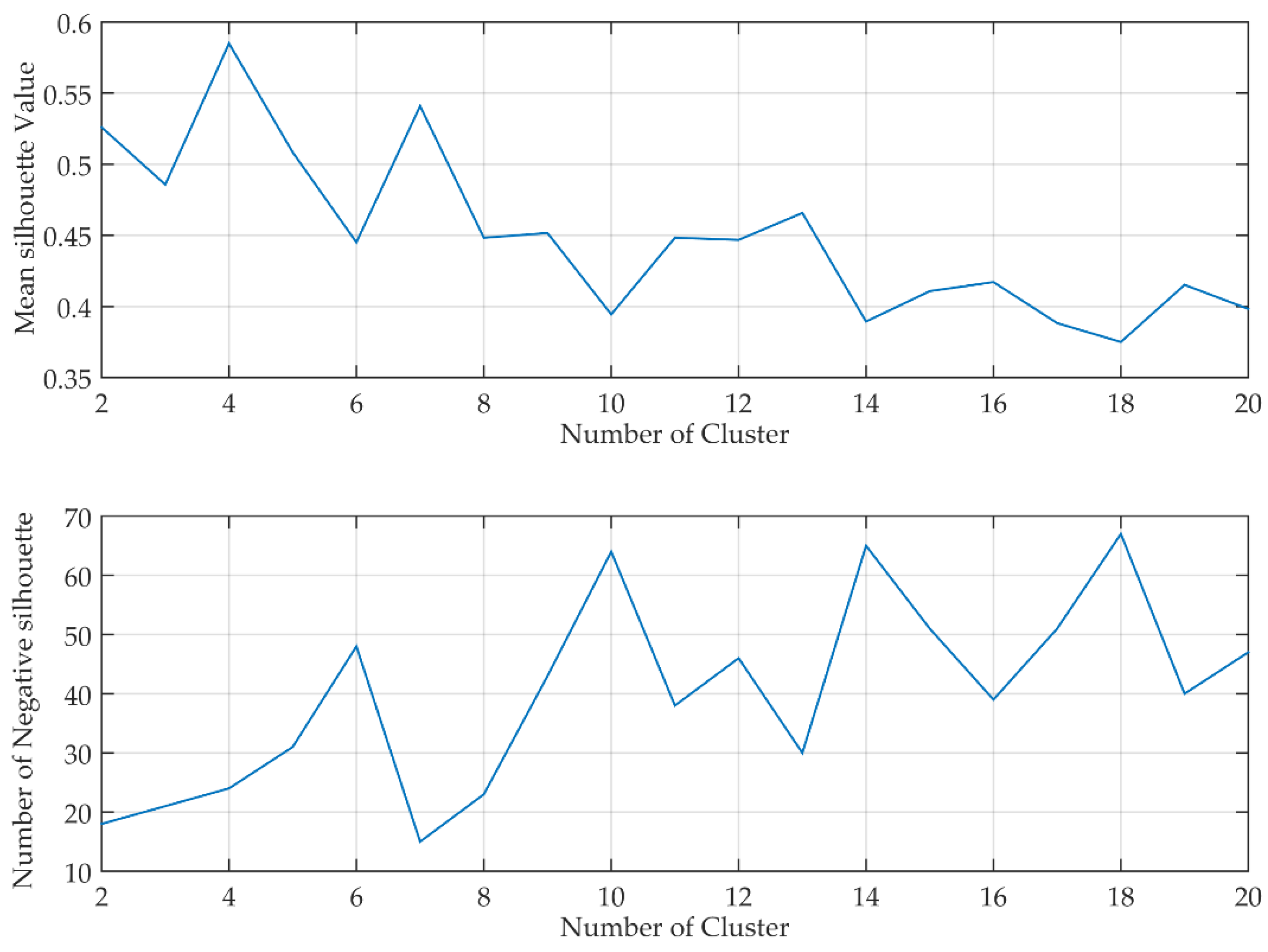
Figure 3.
Genesis location (red circle) and track (green line) of cyclones of four clusters.
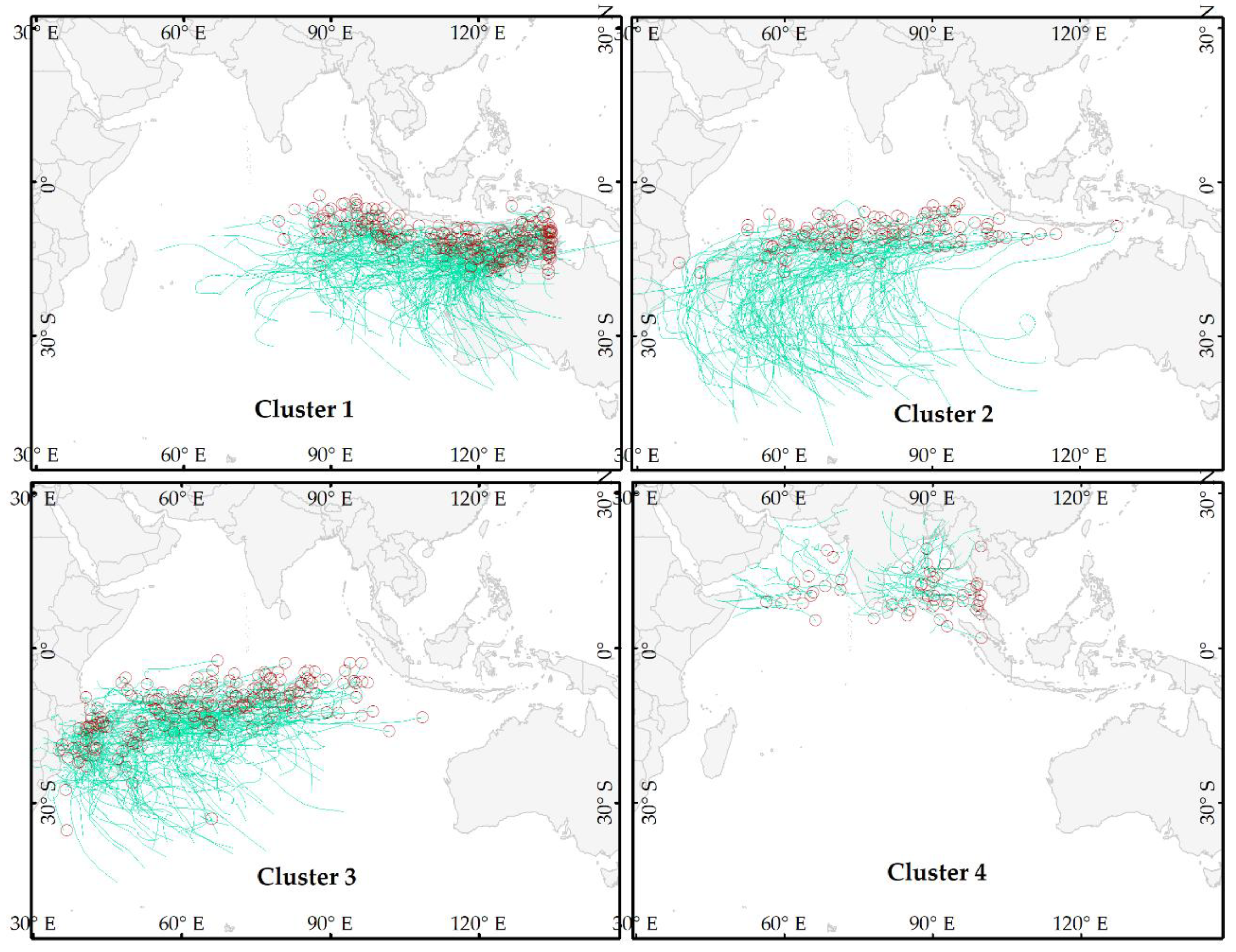
Figure 4.
Cumulative density of genesis location (first position) in each cluster.

Figure 5.
Centroid location (small dots) and standard deviational ellipse (blue) of each cyclone of four clusters. The dark red line shows the mean ellipse and its center (red cross mark) of each cluster.
Figure 5.
Centroid location (small dots) and standard deviational ellipse (blue) of each cyclone of four clusters. The dark red line shows the mean ellipse and its center (red cross mark) of each cluster.

Figure 6.
Box plot of cyclone intensity of cyclones in each cluster and all cyclones. The upper and lower bounds of the box indicate the 75 and 25 percentiles of the distribution, respectively. The mean (diamond mark), median (bar at the middle of the box), and the minimum-maximum bound (dash line) of each cluster are also shown in the figure.

Figure 7.
Box plot of the lifespan of cyclones in each cluster and all cyclones. The upper and lower bounds of the box indicate the 75 and 25 percentiles of the distribution, respectively. The mean (diamond mark), median (bar at the middle of the box), minimum-maximum bound (dash line), and outliers (red plus) of each cluster are also shown in the figure.

Figure 8.
Box plot of track length of cyclones in each cluster and all cyclones. The upper and lower bounds of the box indicate the 75 and 25 percentiles of the distribution, respectively. The mean (diamond mark), median (bar at the middle of the box), minimum-maximum bound (dash line), and outliers (red plus) of each cluster are also shown in the figure.

Figure 9.
Box plot of the rotation angle of deviational ellipses in each cluster and all cyclones. The upper and lower bounds of the box indicate the 75 and 25 percentiles of the distribution, respectively. The mean (diamond mark), median (bar at the middle of the box), minimum-maximum bound (dash line), and outliers (red plus) of each cluster are also shown in the figure.
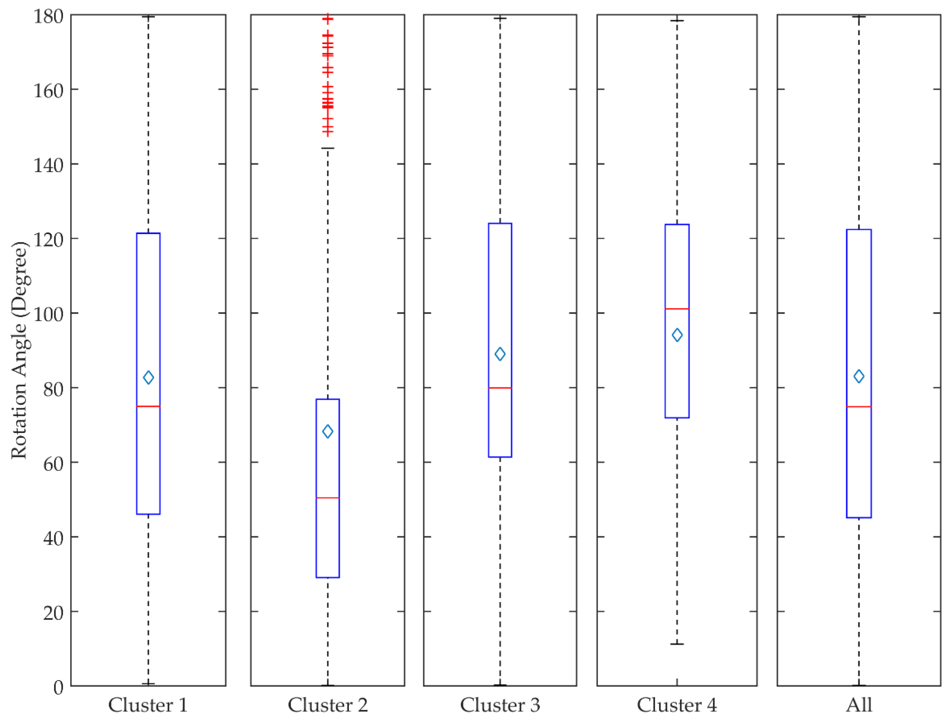
Figure 10.
Box plot of ACE of cyclones in each cluster and all cyclones. The upper and lower bounds of the box indicate the 75 and 25 percentiles of the distribution, respectively. The mean (diamond mark), median (bar at the middle of the box), minimum-maximum bound (dash line), and outliers (red plus) of each cluster are also shown in the figure.
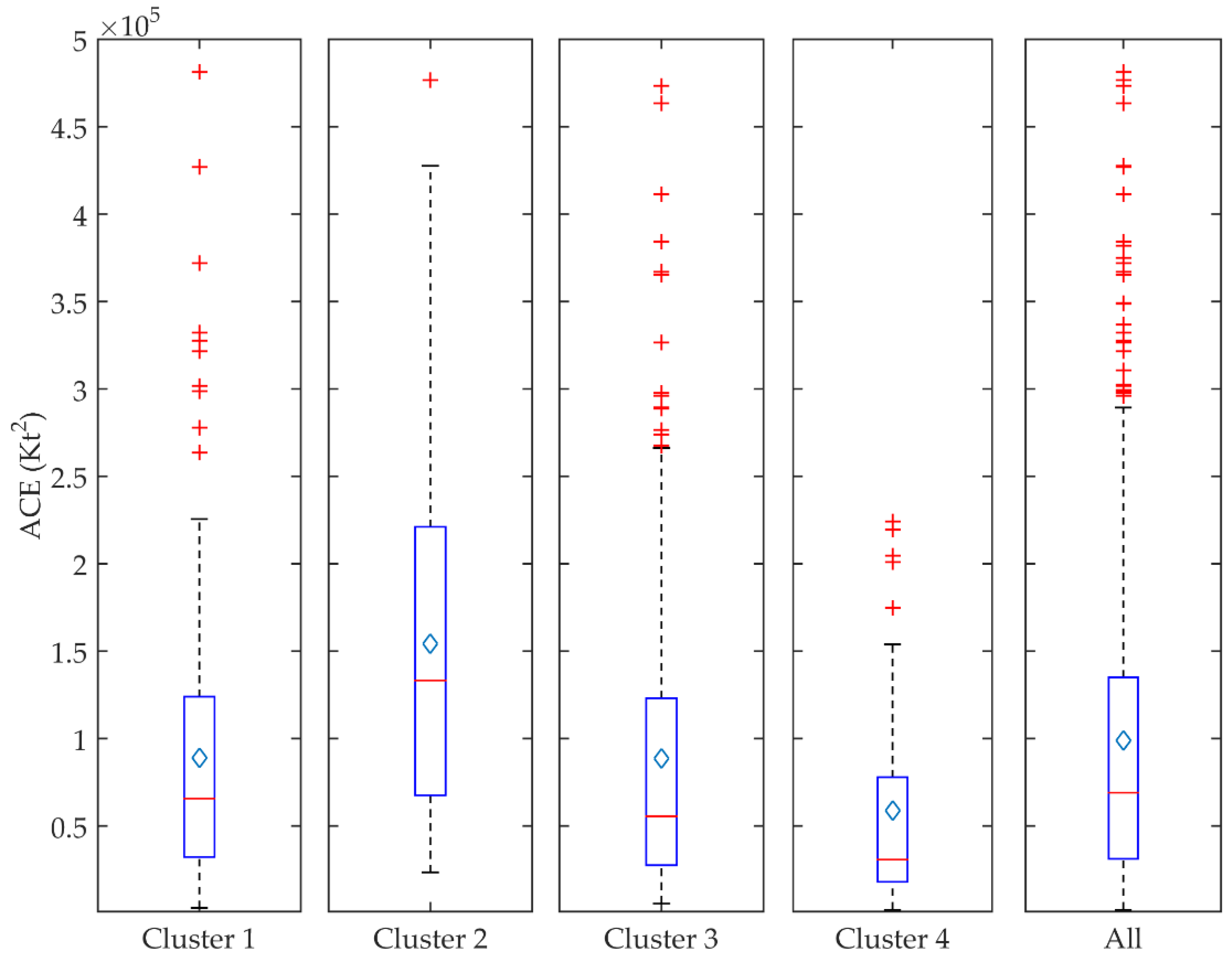
Figure 11.
The relative frequency of TCs by month in each cluster and as a whole.

Figure 12.
Box plot of tropical cyclone month in each cluster and all cyclones. The upper and lower bounds of the box indicate the 75 and 25 percentiles of the distribution, respectively. The mean (diamond mark), median (bar at the middle of the box), minimum-maximum bound (dash line), and outliers (red plus) of each cluster are also shown in the figure.
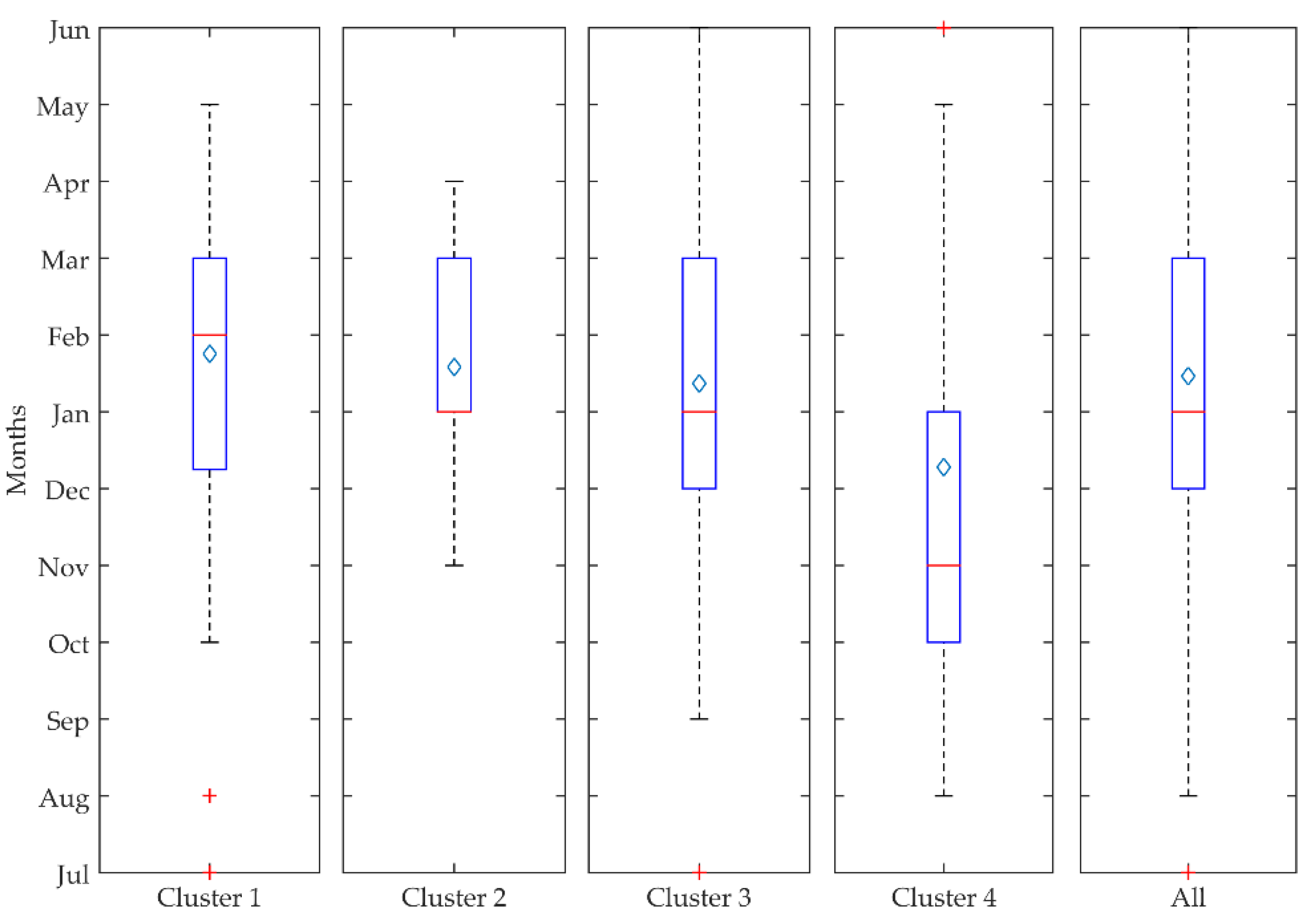
Figure 13.
The landfall locations with the cyclone categories at landfall in each cluster.
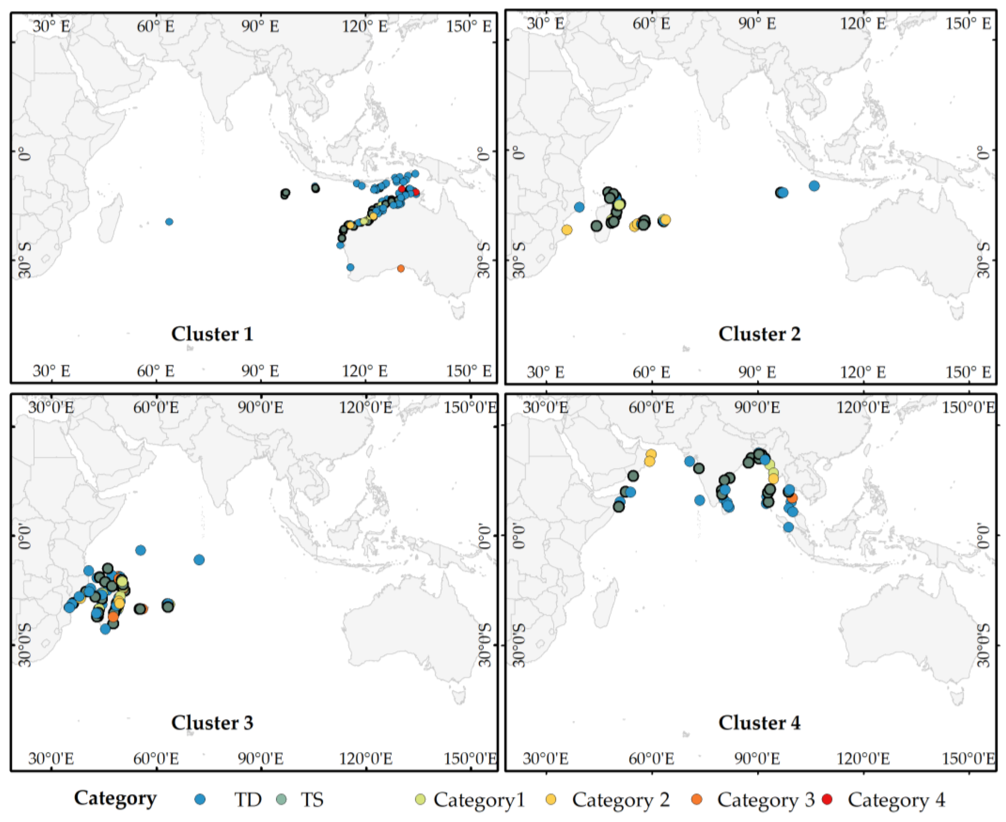
Figure 14.
The number of tropical cyclone per year in each cluster and for all cyclones. Red lines and green lines indicate simple linear regression curves and the curves of Savitzky-Golay filter respectively.
Figure 14.
The number of tropical cyclone per year in each cluster and for all cyclones. Red lines and green lines indicate simple linear regression curves and the curves of Savitzky-Golay filter respectively.
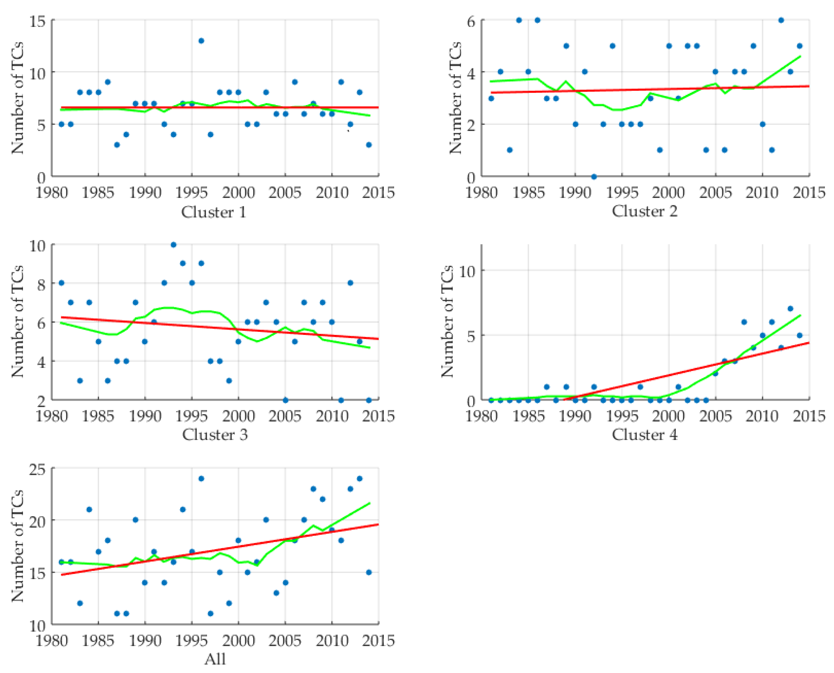
Figure 15.
Accumulated cyclone energy (ACE) per year in each cluster and for all cyclones. Red lines and green lines indicate simple linear regression curves and the curves of Savitzky-Golay filter respectively.
Figure 15.
Accumulated cyclone energy (ACE) per year in each cluster and for all cyclones. Red lines and green lines indicate simple linear regression curves and the curves of Savitzky-Golay filter respectively.
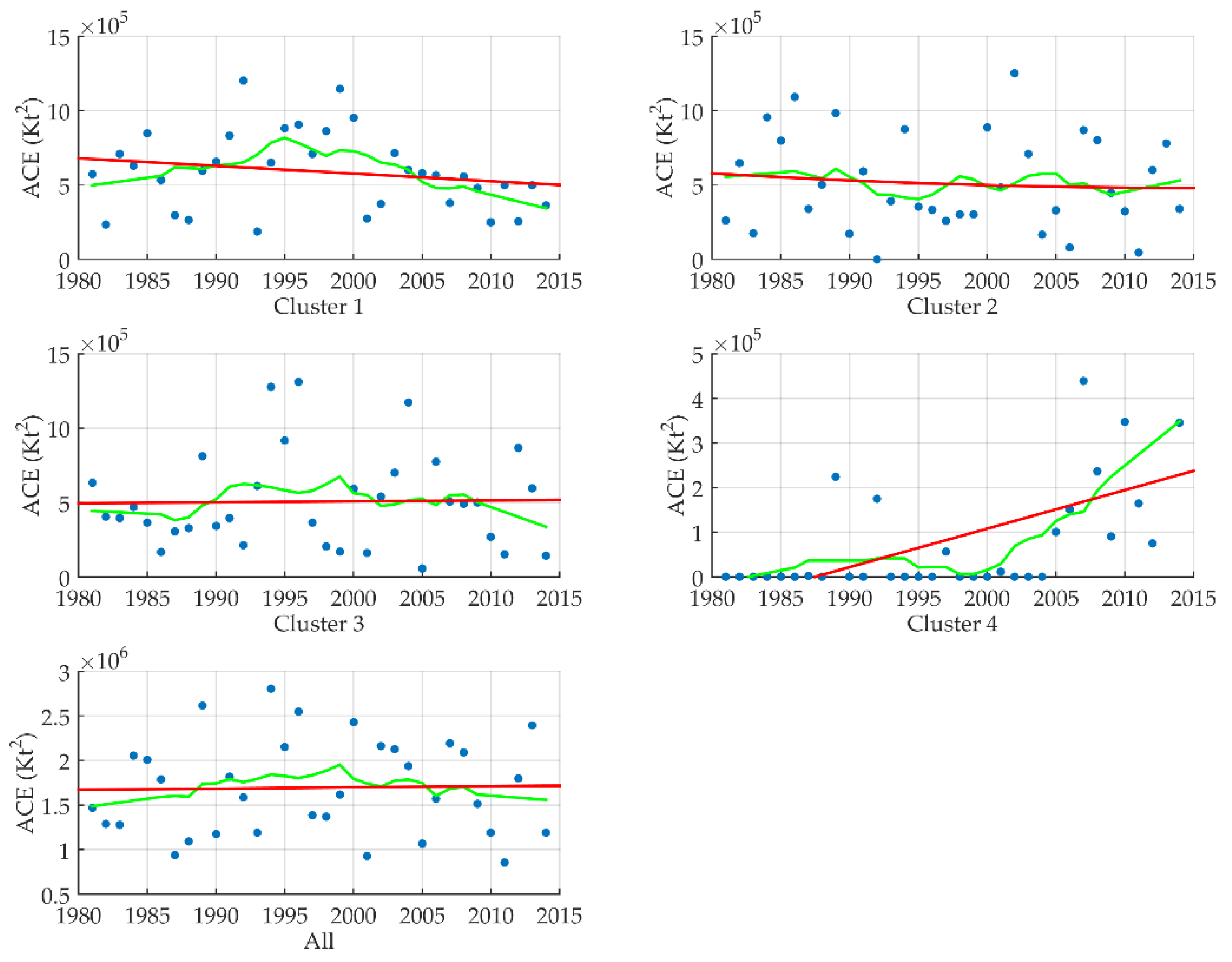
Figure 16.
Composite of daily OLR anomalies two days prior to the TC genesis. The color bar shows the magnitude of the OLR anomalies in Wm−2. Yellow, light green, and dark green contours show the 25, 50, and 75% KDEs of TC genesis locations in each cluster, respectively.
Figure 16.
Composite of daily OLR anomalies two days prior to the TC genesis. The color bar shows the magnitude of the OLR anomalies in Wm−2. Yellow, light green, and dark green contours show the 25, 50, and 75% KDEs of TC genesis locations in each cluster, respectively.

Figure 17.
Box plot of the daily OLR two days prior to TC genesis in each cluster and all TCs. The upper and lower bounds of the box indicate the 75 and 25 percentiles of the distribution, respectively. The mean (diamond mark), median (bar at the middle of the box), and minimum-maximum bound (dash line) of each cluster are also shown in the figure.
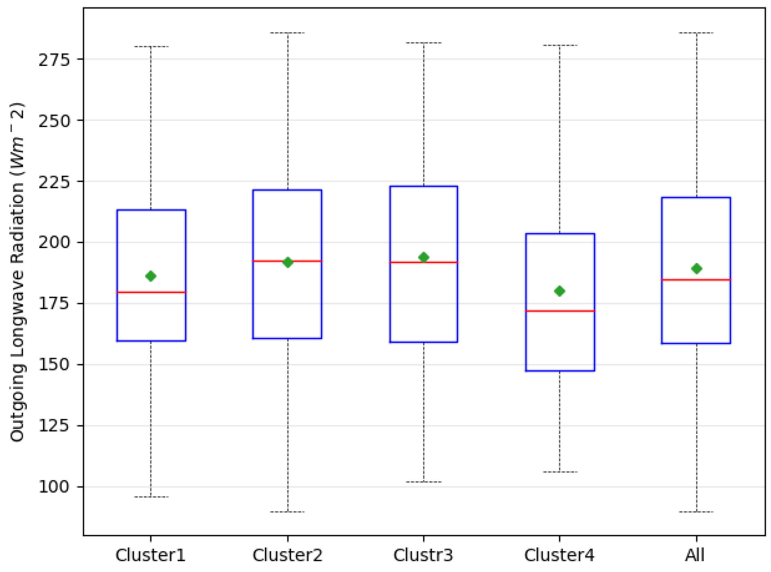
Figure 18.
Composite of weekly SSTA prior to the TC genesis. The color bar shows the magnitude of the SST anomalies in °C. Yellow, light green, and dark green contours show the 25, 50, and 75% KDEs of TCs genesis location in each cluster, respectively.
Figure 18.
Composite of weekly SSTA prior to the TC genesis. The color bar shows the magnitude of the SST anomalies in °C. Yellow, light green, and dark green contours show the 25, 50, and 75% KDEs of TCs genesis location in each cluster, respectively.
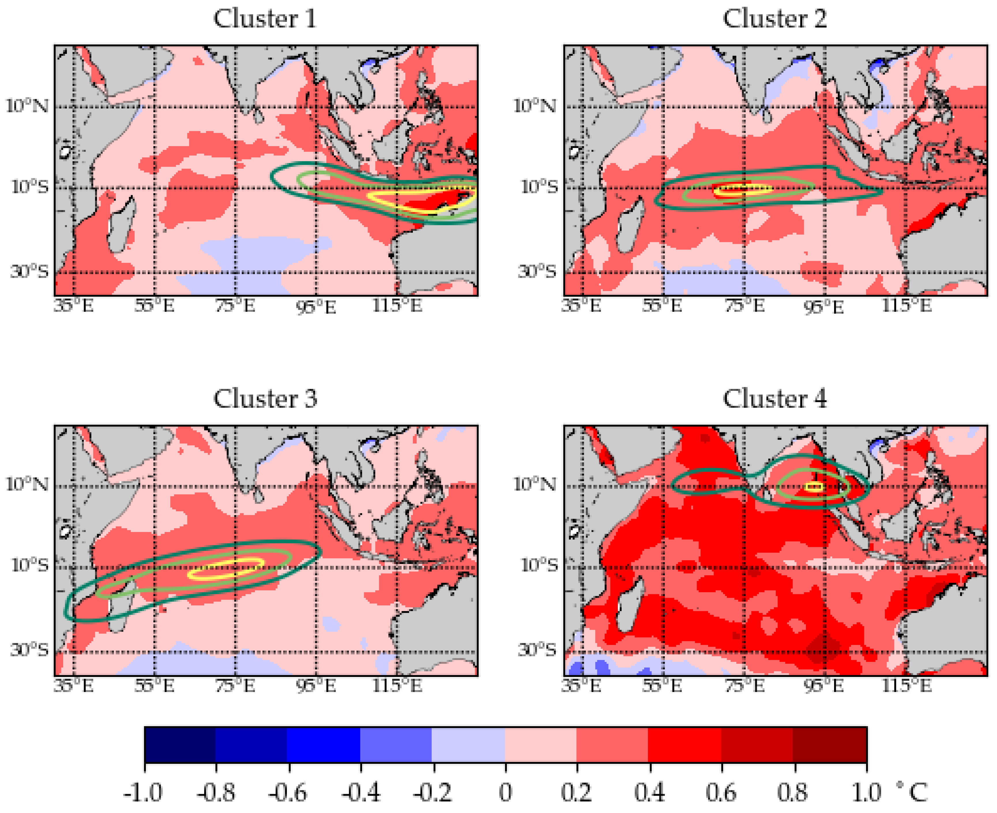
Figure 19.
Box plot of the weekly SST prior to TC genesis in each cluster and all TCs. The upper and lower bounds of the box indicate the 75 and 25 percentiles of the distribution, respectively. The mean (diamond mark), median (bar at the middle of the box), minimum-maximum bound (dash line), and outliers (star marks) of each cluster are also shown in the figure.


Table 1.
Mean and range of cyclone genesis locations of four clusters.
| Clusters | Mean X Genesis | Mean Y Genesis | Genesis X Range | Genesis Y Range | Number of Tracks |
|---|---|---|---|---|---|
| 1 | 115.0° E | 11.4° S | 79.4° E–134.9° E | 2.8° S–19.1° S | 230 |
| 2 | 78.3° E | 10.5° S | 38.0° E–127.0° E | 4.4° S–18.2° S | 116 |
| 3 | 64.7° E | 12.5° S | 35.1° E–108.6° E | 2.5° S–34.7°S | 195 |
| 4 | 84.6° E | 8.6° N | 56.5° E–100.0° E | 2.0° N–20.2° N | 51 |
Table 2.
Mean center, variance, and covariance of the four clusters.
| Cluster No. | Centroid X (° E) | Centroid Y (° N/° S) | Variance X (°) | Variance Y (°) | Variance XY (°) | Number of Tracks |
|---|---|---|---|---|---|---|
| 1 | 110.34° E | 15.58° S | 23.86 | 10.01 | 3.15 | 230 |
| 2 | 67.10° E | 19.40° S | 50.69 | 40.1 | 17.33 | 116 |
| 3 | 59.40° E | 16.77° S | 29.92 | 9.19 | 3.08 | 195 |
| 4 | 79.87° E | 14.01° N | 11.81 | 4.39 | −1.95 | 51 |
Table 3.
Number of cyclones, number of cyclone landfalls, and landfall percentage for each cluster and all cyclones, and the category 1–4 landfall number and percentage.
Table 3.
Number of cyclones, number of cyclone landfalls, and landfall percentage for each cluster and all cyclones, and the category 1–4 landfall number and percentage.
| Cluster | N | Landfalls | Landfall Percentage | Category 1 | Category 2 | Category 3 | Category 4 | Cat 1–4 | |||||
|---|---|---|---|---|---|---|---|---|---|---|---|---|---|
| N | % | N | % | N | % | N | % | N | % | ||||
| 1 | 230 | 119 | 51.73 | 8 | 6.72 | 4 | 3.36 | 2 | 1.68 | 3 | 2.52 | 17 | 14.28 |
| 2 | 116 | 39 | 33.62 | 6 | 15.38 | 6 | 15.38 | 1 | 2.56 | 1 | 2.56 | 14 | 35.89 |
| 3 | 195 | 91 | 46.67 | 11 | 12.09 | 5 | 5.49 | 8 | 8.79 | 1 | 1.1 | 25 | 27.47 |
| 4 | 51 | 43 | 84.31 | 2 | 4.65 | 3 | 6.98 | 1 | 2.33 | 0 | 0.00 | 6 | 13.95 |
| All | 592 | 292 | 49.32 | 27 | 9.25 | 18 | 6.16 | 12 | 4.11 | 5 | 1.71 | 62 | 21.23 |
Table 4.
Statistical significance results of the Kruskal–Wallis tests for TC attributes and environmental variabilities in four clusters.
Table 4.
Statistical significance results of the Kruskal–Wallis tests for TC attributes and environmental variabilities in four clusters.
| Variables | Unit | Cluster 1 | Cluster 2 | Cluster 3 | Cluster 4 | H | p-Value |
|---|---|---|---|---|---|---|---|
| Intensity | knots | 75 | 90 | 63.5 | 52.5 | 39.45 | 0.0001 |
| Rotation angle | Degree | 74.98 | 50.45 | 79.93 | 101.12 | 26.02 | 0.00009 |
| Life span | Days | 7 | 12 | 8 | 5.5 | 121.24 | 0.00000 |
| Track Length | km | 2863 | 5373 | 3245 | 1702 | 183.43 | 0.00000 |
| ACE | Kt2 | 65,652 | 133,247 | 55,550 | 30,737 | 75.57 | 0.00000 |
| SST | °C | 29.27 | 28.78 | 28.61 | 29.00 | 84.59 | 0.00000 |
| OLR | Wm−2 | 179.5 | 192.4 | 192 | 171.9 | 11.73 | 0.0577 |
Table 5.
Statistical significance results of the pairwise Mann–Whitney U tests for TC attributes and environmental variables between cluster pairs.
Table 5.
Statistical significance results of the pairwise Mann–Whitney U tests for TC attributes and environmental variables between cluster pairs.
| Clusters | C1 | C2 | C2 | C3 | C3 | C4 | C1 | C3 | C1 | C4 | C2 | C4 | |
|---|---|---|---|---|---|---|---|---|---|---|---|---|---|
| U | p | U | p | U | p | U | p | U | p | U | p | ||
| Variables | Intensity | 9772 | 0.000 | 6827 | 0.00 | 4121 | 0.079 | 18,516 | 0.002 | 4197 | 0.001 | 1590 | 0.00 |
| Rotation angle | 9965 | 0.000 | 7256 | 0.00 | 4277 | 0.099 | 19,717 | 0.046 | 4699 | 0.029 | 1985 | 0.00 | |
| Life span | 5043 | 0.000 | 6172 | 0.00 | 2376 | 0.000 | 18,690 | 0.004 | 3320 | 0.000 | 319 | 0.00 | |
| Track Length | 3210 | 0.000 | 3578 | 0.00 | 2163 | 0.000 | 19,671 | 0.030 | 2829 | 0.000 | 69 | 0.00 | |
| Seasonality | 9679 | 0.000 | 8361 | 0.00 | 2448 | 0.000 | 21,692 | 0.395 | 2556 | 0.000 | 917 | 0.00 | |
| ACE | 7011 | 0.000 | 5689 | 0.00 | 3649 | 0.004 | 20,503 | 0.112 | 3907 | 0.000 | 933 | 0.00 | |
| SST | 7622 | 0.000 | 8779 | 0.007 | 3234 | 0.000 | 10,800 | 0.000 | 4566 | 0.011 | 2308 | 0.02 | |
| OLR | 12,023 | 0.067 | 11,188 | 0.437 | 4034 | 0.019 | 20,006 | 0.028 | 5221 | 0.110 | 2406 | 0.03 |
Note: All values are statistically significant at α = 0.05 except values in bold.
© 2018 by the authors. Licensee MDPI, Basel, Switzerland. This article is an open access article distributed under the terms and conditions of the Creative Commons Attribution (CC BY) license (http://creativecommons.org/licenses/by/4.0/).
Share and Cite
MDPI and ACS Style
Rahman, M.S.; Yang, R.; Di, L. Clustering Indian Ocean Tropical Cyclone Tracks by the Standard Deviational Ellipse. Climate 2018, 6, 39. https://doi.org/10.3390/cli6020039
AMA Style
Rahman MS, Yang R, Di L. Clustering Indian Ocean Tropical Cyclone Tracks by the Standard Deviational Ellipse. Climate. 2018; 6(2):39. https://doi.org/10.3390/cli6020039
Chicago/Turabian StyleRahman, Md. Shahinoor, Ruixin Yang, and Liping Di. 2018. "Clustering Indian Ocean Tropical Cyclone Tracks by the Standard Deviational Ellipse" Climate 6, no. 2: 39. https://doi.org/10.3390/cli6020039
Note that from the first issue of 2016, this journal uses article numbers instead of page numbers. See further details here.