Hydrological Modeling in Northern Tunisia with Regional Climate Model Outputs: Performance Evaluation and Bias-Correction in Present Climate Conditions

Abstract

This work aims to evaluate the performance of a hydrological balance model in a watershed located in northern Tunisia (wadi Sejnane, 378 km²) in present climate conditions using input variables provided by four regional climate models. A modified version (MBBH) of the lumped and single layer surface model BBH (Bucket with Bottom Hole model, in which pedo-transfer parameters estimated using watershed physiographic characteristics are introduced) is adopted to simulate the water balance components. Only two parameters representing respectively the water retention capacity of the soil and the vegetation resistance to evapotranspiration are calibrated using rainfall-runoff data. The evaluation criterions for the MBBH model calibration are: relative bias, mean square error and the ratio of mean actual evapotranspiration to mean potential evapotranspiration. Daily air temperature, rainfall and runoff observations are available from 1960 to 1984. The period 1960–1971 is selected for calibration while the period 1972–1984 is chosen for validation. Air temperature and precipitation series are provided by four regional climate models (DMI, ARP, SMH and ICT) from the European program ENSEMBLES, forced by two global climate models (GCM): ECHAM and ARPEGE. The regional climate model outputs (precipitation and air temperature) are compared to the observations in terms of statistical distribution. The analysis was performed at the seasonal scale for precipitation. We found out that RCM precipitation must be corrected before being introduced as MBBH inputs. Thus, a non-parametric quantile-quantile bias correction method together with a dry day correction is employed. Finally, simulated runoff generated using corrected precipitation from the regional climate model SMH is found the most acceptable by comparison with runoff simulated using observed precipitation data, to reproduce the temporal variability of mean monthly runoff. The SMH model is the most accurate to reproduce the occurrence of dry days but still underestimates them. From the statistical distribution point of view, corrected SMH precipitation data introduced into the MBBH model were not able to reproduce extreme runoff values generated by observed precipitation data during validation (larger than 80 mm/month). This may be due to the SMH weakness in reproducing moderate and high rainfall levels even after bias correction. This approach may be considered as a way to use regional climate models (RCM) model outputs for studying hydrological impacts.

1. Introduction

Mediterranean countries, such as Tunisia, are in the transition zone between the semi-arid climate of North Africa and the temperate and rainy climate of Central Europe. They are highly vulnerable to climate change as previously reported in several studies [1,2,3]. In Tunisia, most of the dams and reservoirs used in the management of water resources are located in the northern part of the country. This makes it important to consider the likely consequences of climate change on this resource. In particular, future climate projections for this area indicate a decrease in precipitation by 20% [4]. Such projections stress the need for impact studies at the basin scale, which is the relevant scale for water resource management and mitigation strategies.

The most common approach to estimate climate change impacts on water resources is to combine climate model outputs with hydrological models [5,6,7]. However, due to the coarse resolution of Global Circulation Models (GCM), their outputs need to be downscaled to match the scale of interest for an impact study [8]. In recent years, several ensembles of regional climate models (RCM) outputs, such as ENSEMBLES [9], have been developed by the climate scientist community to provide model outputs at a scale compatible with basin-scale studies. One advantage of RCMs over GCMs is that they more accurately take into account orography, thus providing a better reproduction of regional climates. In addition, they do not require to be calibrated with ground data, as for statistical downscaling methods. However, despite the recent improvements to increase their resolution, their outputs are often affected by a strong systematic bias [8,9,10,11,12,13,14].

The goal of this study is to evaluate different runs of RCMs for a medium-scale catchment located in northern Tunisia for hydrological modeling purpose. A hydrological model is first set-up with the available hydro-meteorological data. Then, the outputs of different RCMs from the ENSEMBLES project are compared with observations, and finally they are tested after bias correction as inputs of the hydrological model to evaluate their ability to reproduce observed runoff dynamics. Hydro-climatic data and selected RCMs are presented in Section 2, followed by the methodology in Section 3, where the hydrological model and its calibration method are presented as well as the RCM bias correction method. In Section 4, model calibration and validation results are reported as well as the hydrological impacts of corrected RCM precipitation series in terms of runoff.

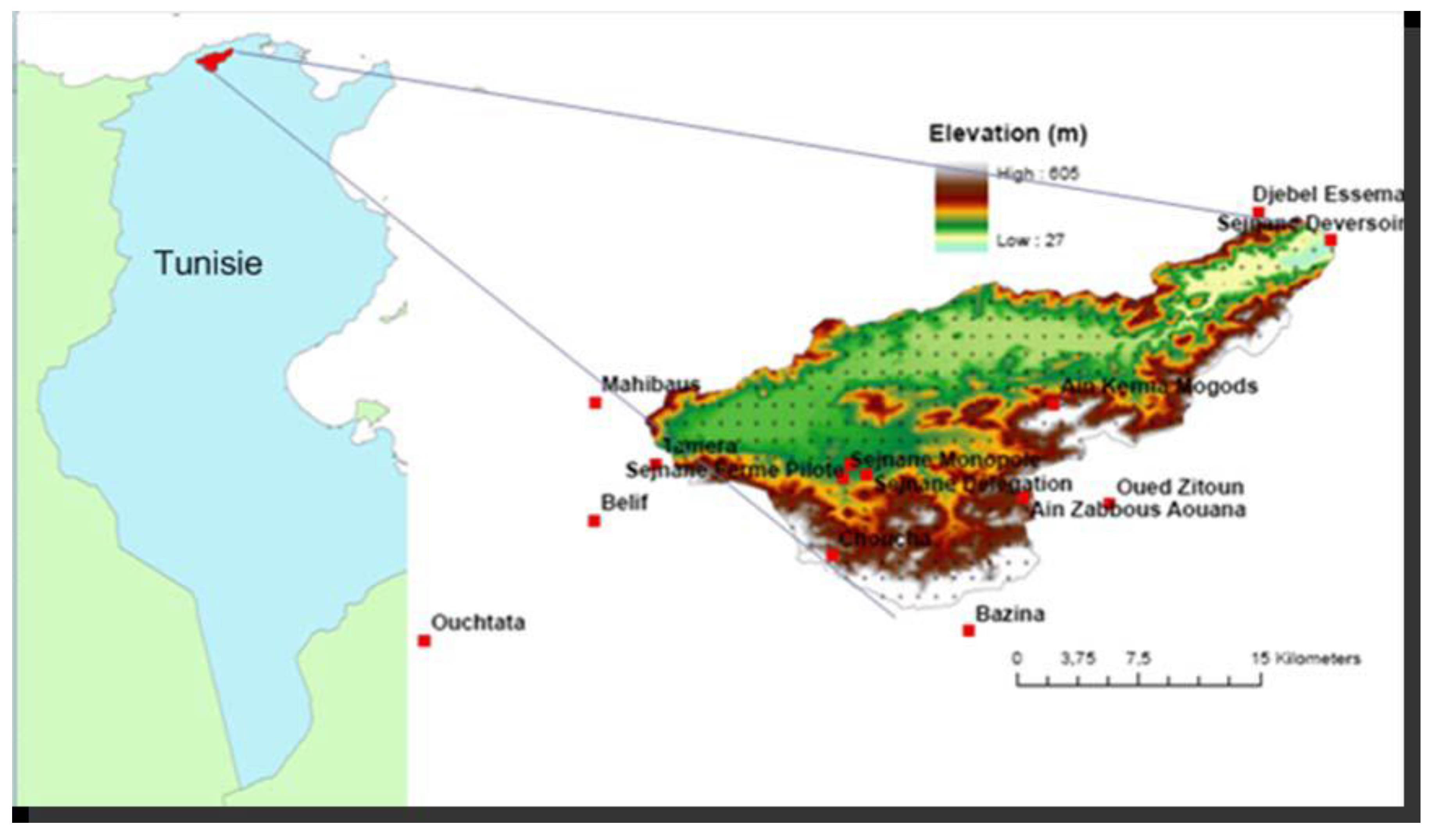
2. Study Area and Data

The study area is located between 36°N and 38°N and 7°E and 8°E (Figure 1). Characterized by a semi-arid climate, it covers an area of 378 km². It is constituted by the upper Wadi Sejnane watershed controlled by a hydrometric station named Sejnane Déversoir. Wadi Sejnane flows over 33.5 km, feeding the freshwater Lake Ichkeul which is its final outlet [15]. The latter is a humid zone recognized as a World Heritage Site (United Nations Environment Programme-World Conservation M [16]). In the watershed controlled by the hydrometric station, elevations range from 27 m to 605 m (Figure 1). The relief is rugged. Watershed occupation is mainly annual dry crops (22%), hardwood forest (17%) and meadows (13%) as well as olives (13%). Urbanized areas represent only 2% of the basin. Nowadays, a dam located downstream with respect to the location of the hydrometric station controls river discharge directly. This dam supplies water for domestic and agricultural uses at the local and regional levels. Part of the water storage is transferred to Tunis City located more than one hundred kilometers from the dam site.

Figure 1. Localization of the study area with rainfall stations network.

Figure 1. Localization of the study area with rainfall stations network.

2.1. Ground Hydro-Climatic Data

Monthly air temperature data are provided by the Tunisian meteorological service (INM) collected from the nearest meteorological stations (Bizerte, Béja, Tabarka) in such a way that the study period 1960–2010 is covered (Figure 1). Data reflect the well-known Mediterranean seasonal effect with a hot summer and a mild winter. Potential evapotranspiration (PET) is estimated using the Oudin empirical formula [17] which requires only air temperature observations.

The daily precipitation database is provided by the national hydrological service (DGRE) and contains 14 rain gauge stations. Observations cover the study period 1960–2010. We considered hydrological years that start on September 1st and end on August 31th. Station locations are reported in Figure 1. Only six stations are inside the basin. As the database contains some gaps, to compute the mean areal rainfall over the watershed by the Thiessen interpolation method, weights are estimated day by day, according to data availability. Mean monthly precipitation variability shows a humid season (September to April) well identified compared to a dry season (May to August), which represents one of the characteristics of the Mediterranean climate.

The mean daily flow time series covers the sub-period 1960–1994 at the gauging station Sejnane déversoir (Figure 1). After 1994, the dam was built and the station was removed. The measurements were kindly provided by the national hydrological service DGRE.

2.2. Regional Climate Models Data

Four different RCM simulation runs at the 25 km spatial resolution of precipitation and air temperature were extracted from the European project ENSEMBLES [18]. The RCM runs included in this study are those of the French meteorological service [19], the Danish Meteorological Institute [20], the International Center for Theoretical Physics in Trieste, Italy [21] and the Swedish Meteorological and Hydrological Institute SMHI [22]. These RCMs are driven by two different general circulation models (GCM): The Max Planck Institute ECHAM model (for SMH and ICT) and the ARPEGE model developed in Météo-France (for ARP and DMI).

3. Methodology

3.1. Hydrological Modeling

A modified version (noted MBBH) of the daily hydrological model BBH [23] was used. This modified version was proposed by [24]. The daily model involves a single active soil layer which defines the root zone. As an input series, the BBH model use daily potential evapotranspiration and rainfall and its outputs are actual evapotranspiration, surface runoff, capillary rise, percolation, daily soil moisture and the average soil water content.

The model has seven parameters: p, the parameter representing soil porosity, D, the parameter representing active soil layer depth (mm), Ks, the parameter representing hydraulic conductivity at the surface (mm/j), SFC, the parameter representing the soil field capacity, B, the parameter representing the soil retention curve form, η, the parameter representing the capacity of water retention, and σ, the parameter representing the vegetation resistance to evapotranspiration. The model is lumped which means that parameters are assumed homogeneous over the basin area.

Based on a soil texture map obtained from the Forestry department of the Agriculture Ministry and the USDA textural triangle norm, we deduced that the main soil texture is silty clay. Ks and SFC are estimated for every soil texture using pedo-transfer functions from the model proposed in [25]. Spatial averages are computed using weights with respect to the area covered by a given soil texture. The resulting parameter estimates are Ks = 213 mm/d and SFC = 0.45. The value p = 0.48 is taken to represent the silty clay soil texture. Based on the work in [26], we take B = 9. After different calibration trials, the parameter D is fixed at D = 500 mm, which seems coherent with respect to vegetation and soil texture. Another assumption is that no capillary rise occurs. Parameters η and σ were calibrated using series of mean average rainfall and potential evapotranspiration (in mm/d) and observations of surface runoff (in mm/d). The interval of variation of both η and σ search is [0, 1] and is scanned by steps of 0.01.

The ratio of mean annual actual evapotranspiration to mean annual potential evapotranspiration is adopted to assess the adequacy of hydrological model. Proposed by [27], this ratio, denoted Kv, reflects information about vegetation. For the Sejnane basin, which belongs to a sub humid type area of Tunisia, we assume that the Kv ratio should range between 0.45 and 0.55. Consequently, three criteria are considered hierarchically to achieve model fitting: (i) the relative bias of the total flow over the calibration period must be less than 5%, (ii) the root mean square error (RMSE) of the monthly flows is minimized and (iii) the Kv ratio must fulfill the condition 0.45 < Kv < 0.55 which reflects that the selected solution is adequate with ecosystem characteristics. Finally, the Nash coefficient and the volume bias are also calculated to evaluate the results both in calibration and validation. The calibration period is 1960–1971 and the validation period is 1972–1984. Note that runoff data are missing from October 1976 to May 1977.

3.2. RCM Outputs Evaluation

Before being used as model inputs in MBBH, the outputs of climate models (precipitation and air temperature series) are analyzed and compared to observations. To this aim, attention is paid to (a) the reproduction of the rainfall seasonal cycles and (b) the good matching between observed ground data distributions and simulated RCM outputs distributions. The control period is 11 years from 1 September 1960 to 31 August 1971. The validation period is 13 years from 1 September 1971 to 31 August 1984. The distribution comparison is performed with the Kolmogorov-Smirnov (K-S) and Cramer-von Mises (CvM) non parametric tests [28].

3.3. Correction of the RCM outputs

The bias-correction of precipitation simulated by the RCMs is performed at the daily scale for each season to ensure the homogeneity of the cumulative distribution functions (CDF). Among the existing bias-correction methods, a quantile-quantile approach is chosen [13,29]. In order to choose between parametric or non-parametric quantile-quantile methods, the adequacy of Gamma distribution for fitting daily rainfall series is tested. At the 95% confidence level, it was found that, for precipitation data in the autumn season (from September to November SON) and in the spring season (from March to May MAM), the Kolmogorov-Smirnov adequacy test rejects the null hypothesis of a Gamma distribution. Thus, a non-parametric quantile-quantile method, the so-called CDFt method proposed by [30] for wind series correction and applied to temperature and rainfall by [31] is employed. The CDFt method consists of a transformation that is applied to the simulated daily precipitation distribution to obtain a distribution which matches the distribution of the observations.

3.4. Drizzle Day Correction

It is well known that RCMs produce too many drizzle days; i.e., rain events less than a few millimeters that are not obtained by measurement devices. This results in the overestimation of the number of rainy days by RCM models. We implemented a correction to account for this called dry day correction.

As in [32], two correction approaches are investigated. Firstly, a fixed threshold of 1 mm/day is assumed and each RCM rain value that does not exceed 1 mm/day is redefined to zero. The second approach is to assume the conservation of the number of observed dry days in the observed and simulated series. Thus, a threshold is identified so that the number of dry days (in the control period) is similar for both observed and RCM simulated series.

4. Results

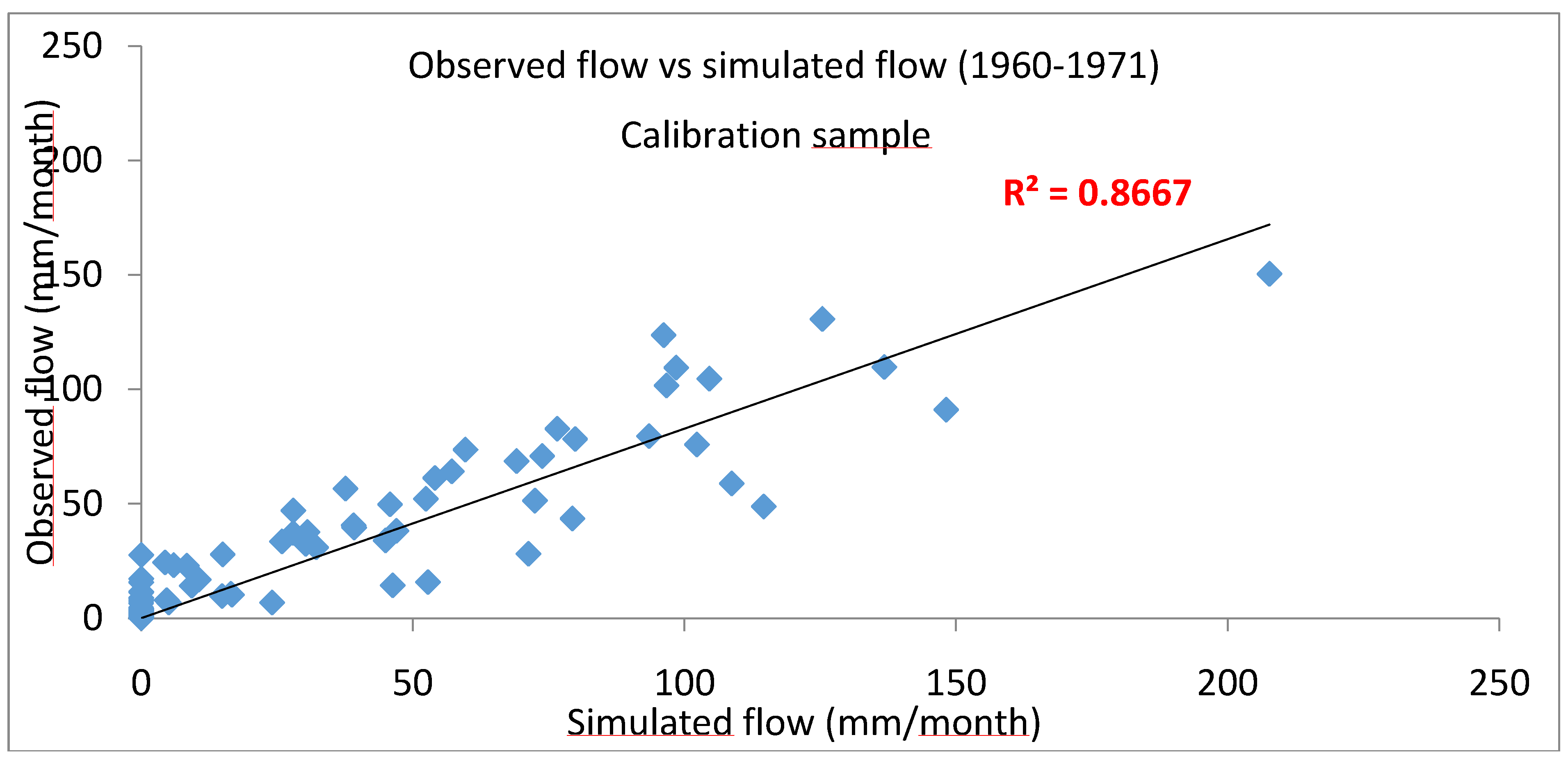
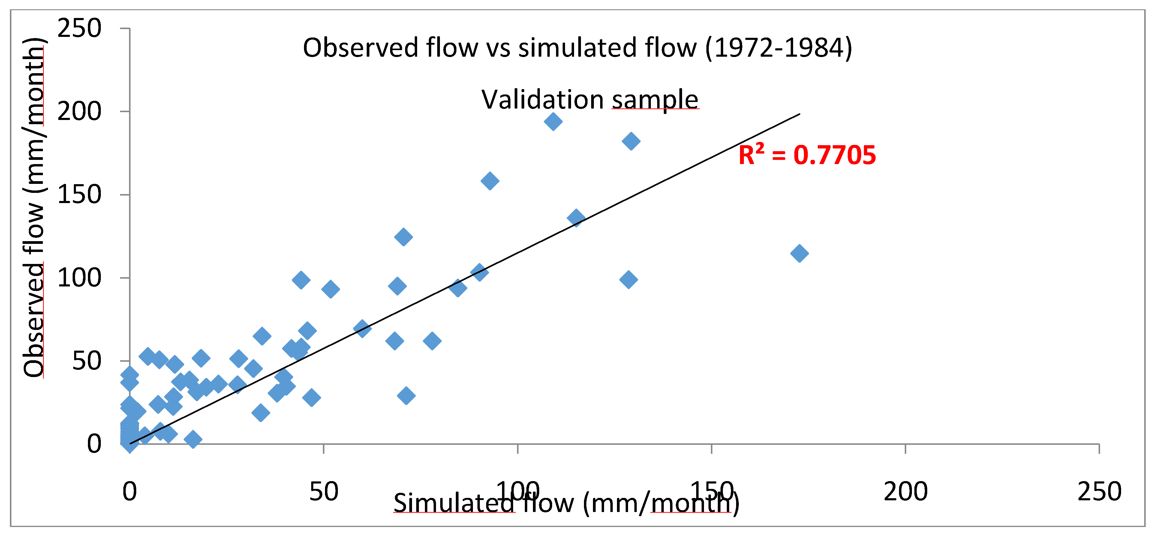
4.1. Hydrological Model Calibration Result Using Ground Data

The calibration of the hydrological model was performed over the period 1960–1971 (the control period) and the evaluation was carried out on the period 1972–1984 (the validation period). Table 1 reports calibrated model parameters as well as evaluation criteria.

Table 1. Model parameters and quality criteria.

η	σ	Monthly RMSE (Calibration)	Decadal RMSE (Calibration)	Monthly RMSE(Validation)	Decadal RMSE (Validation)
0.53	0.14	14.7	3.1	15.9	3.3

Table 1. Model parameters and quality criteria.

η	σ	Monthly RMSE (Calibration)	Decadal RMSE (Calibration)	Monthly RMSE(Validation)	Decadal RMSE (Validation)
0.53	0.14	14.7	3.1	15.9	3.3

Figure 2. Scatter plot of observed and predicted monthly runoff for calibration data.

Figure 2. Scatter plot of observed and predicted monthly runoff for calibration data.

Figure 2 and Figure 3 show the scatter plots of observed and simulated monthly runoff. The correlation between simulated and observed flows during the calibration period is satisfactory as shown by the value of the coefficient of determination (R² = 0.87). Moreover, the model can reproduce high monthly values and keeps a good performance (R² = 0.77) during the validation period. Although the Nash is deteriorated from 0.81 for the calibration period to 0.71 during the validation period, this score remains acceptable.

The calibrated MBBH model simulates monthly flows that are synchronous with the observed flows. The model reproduces adequately monthly flows during the calibration period (within the margin defined beforehand by the criterion of maximum 5% relative bias on the total flow). However, during the period of validation, the three largest monthly totals (from 160 to 180 mm/month) are underestimated resulting in −31.6% of runoff underestimation for the entire validation period while total runoff was overestimated by +4.8% for the calibration period. Despite these shortcomings, the calibrated model is adopted for subsequent analysis.

Figure 3. Scatter plot of observed and predicted monthly runoff for validation data.

Figure 3. Scatter plot of observed and predicted monthly runoff for validation data.

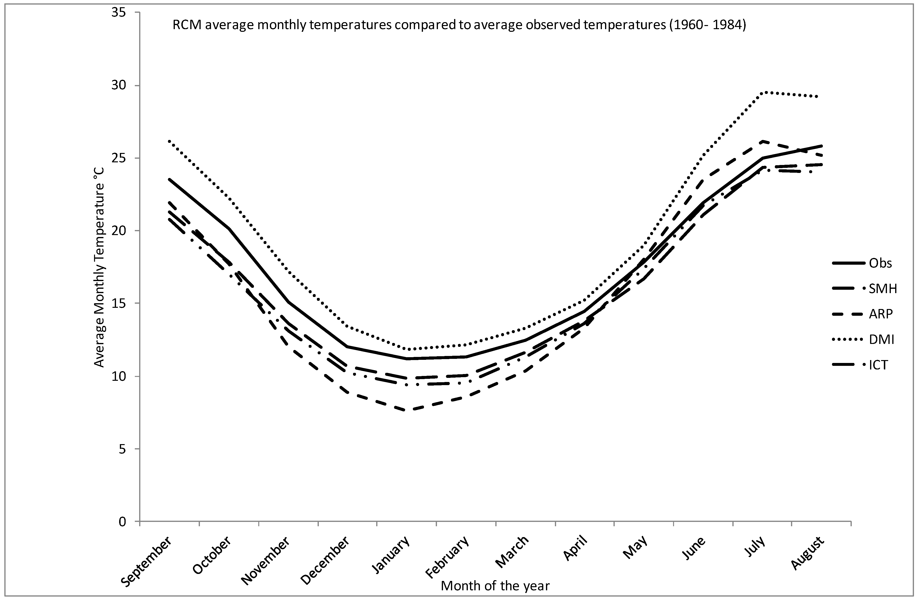
4.2. Evaluation of RCM Simulated Air Temperature

Monthly air temperature regimes are shown in Figure 4 for both observed and RCM data.

Mean monthly air temperatures estimated using the period 1960–1984 are more accurately reproduced in cold months than it hot months (summer season) (Figure 4).

The most accurate RCM in the winter season (DJF) is DMI, while the most accurate in summer season (JJA) is ICT (Table 2). The RCMs that are forced by the same GCM present similar simulations especially SMH and ICT. The comparison between daily PET estimations computed with observed air temperature series on one hand and with RCM simulated air temperature series on the other hand, shows acceptable similarities, especially for DMI and SMH. Consequently, in the following, RCM simulated air temperatures are adopted for PET estimation without correction.

The MBBH model was recalibrated with the PET estimated using the non-corrected RCM air temperature data. It was found that model accuracy is not very sensitive to the PET input as shown by the range of variation in Nash and Kv values: 0.81 < Nash < 0.89 and 0.45 < Kv < 0.48 which is similar to the performances obtained using observed PET. This may support the idea that air temperature correction might be not needed for this study.

Figure 4. Seasonal variability of monthly air temperature (observed and RCM outputs).

Figure 4. Seasonal variability of monthly air temperature (observed and RCM outputs).

Table 2. Regional climate model (RCM) error in monthly average temperature (°C) (1960–1984).

Monthly Temp. Bias	SMH	ARP	DMI	ICT
September	2.3	1.6	−2.6	2.8
October	2.3	2.4	−2.1	3.1
November	1.5	3.1	−2.1	2.0
December	1.3	3.1	−1.5	1.8
January	1.3	3.6	−0.7	1.8
February	1.3	2.8	−0.8	1.8
March	0.8	2.1	−0.8	1.1
April	0.7	1.1	−0.8	0.8
May	1.1	−0.2	−1.1	0.5
June	0.8	−1.6	−3.3	0.2
July	0.7	−1.1	−4.6	0.8
August	1.3	0.7	−3.4	1.8

Table 2. Regional climate model (RCM) error in monthly average temperature (°C) (1960–1984).

Monthly Temp. Bias	SMH	ARP	DMI	ICT
September	2.3	1.6	−2.6	2.8
October	2.3	2.4	−2.1	3.1
November	1.5	3.1	−2.1	2.0
December	1.3	3.1	−1.5	1.8
January	1.3	3.6	−0.7	1.8
February	1.3	2.8	−0.8	1.8
March	0.8	2.1	−0.8	1.1
April	0.7	1.1	−0.8	0.8
May	1.1	−0.2	−1.1	0.5
June	0.8	−1.6	−3.3	0.2
July	0.7	−1.1	−4.6	0.8
August	1.3	0.7	−3.4	1.8

However, it is found that the new calibrated parameter σ is changed, while the parameter η remains unchanged (0.53 < η < 0.54). With observed PET, calibration resulted in σ = 0.14 while using non corrected air temperature series it resulted to σ = 0.01. Note that the stomatal resistance parameter σ is supposed to be high where climate and soil humidity conditions are unfavorable and weak when they are favorable. This result may suggest that using the non-corrected air temperature series results in higher soil humidity conditions than in real situations. Thus, despite the closeness of monthly PET averages computed with observed and non-corrected RCM air temperatures, other statistical features such as air temperature variance and serial correlation may impact the final estimation of the parameter σ representing the vegetation resistance to evapotranspiration (vegetation response). This is a very interesting outcome reflecting the complexity of the problem: Observed air temperature series and non-corrected RCM air temperature series are not translated into the same vegetation response features while they give similar predictions for runoff.

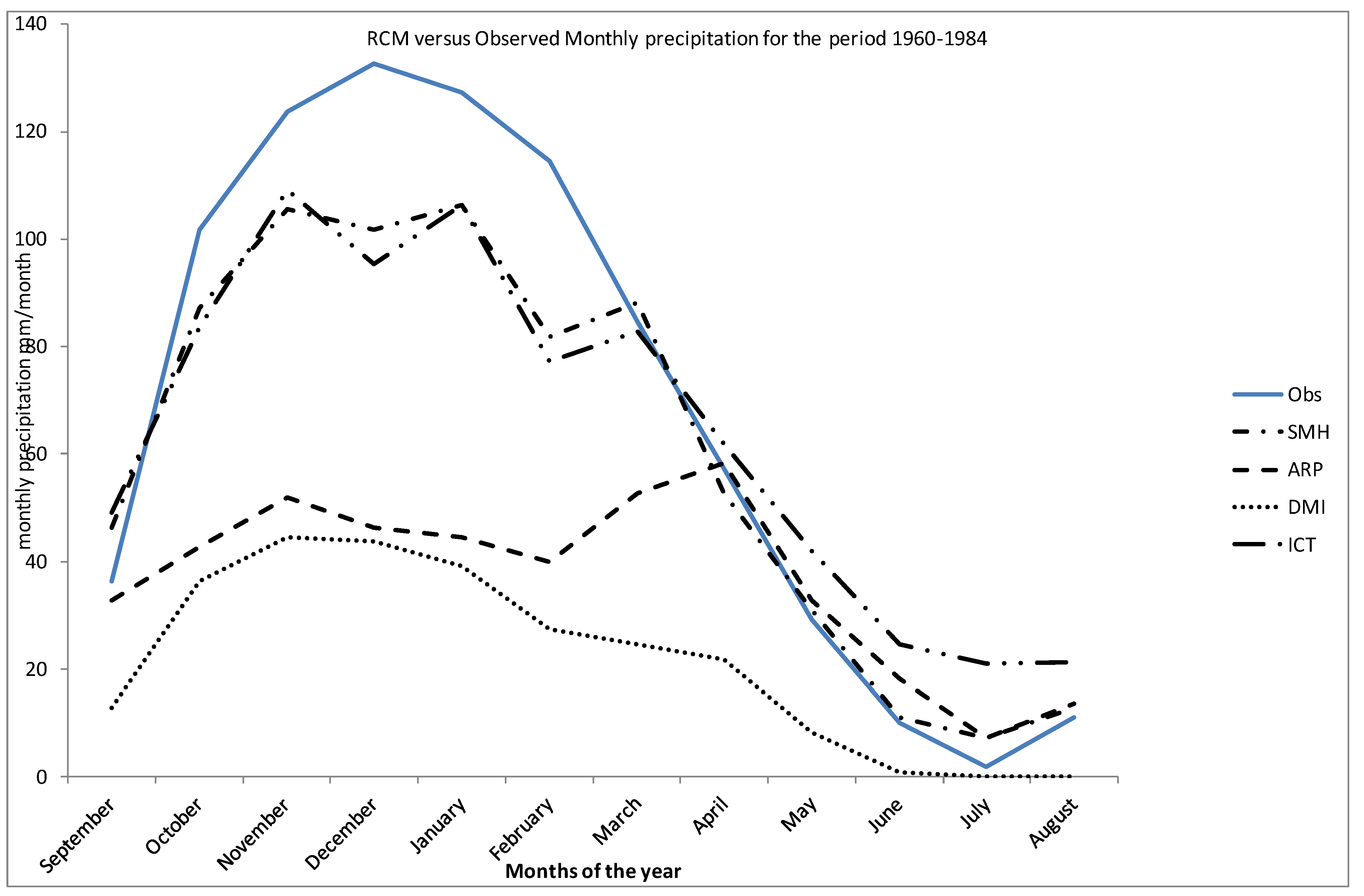
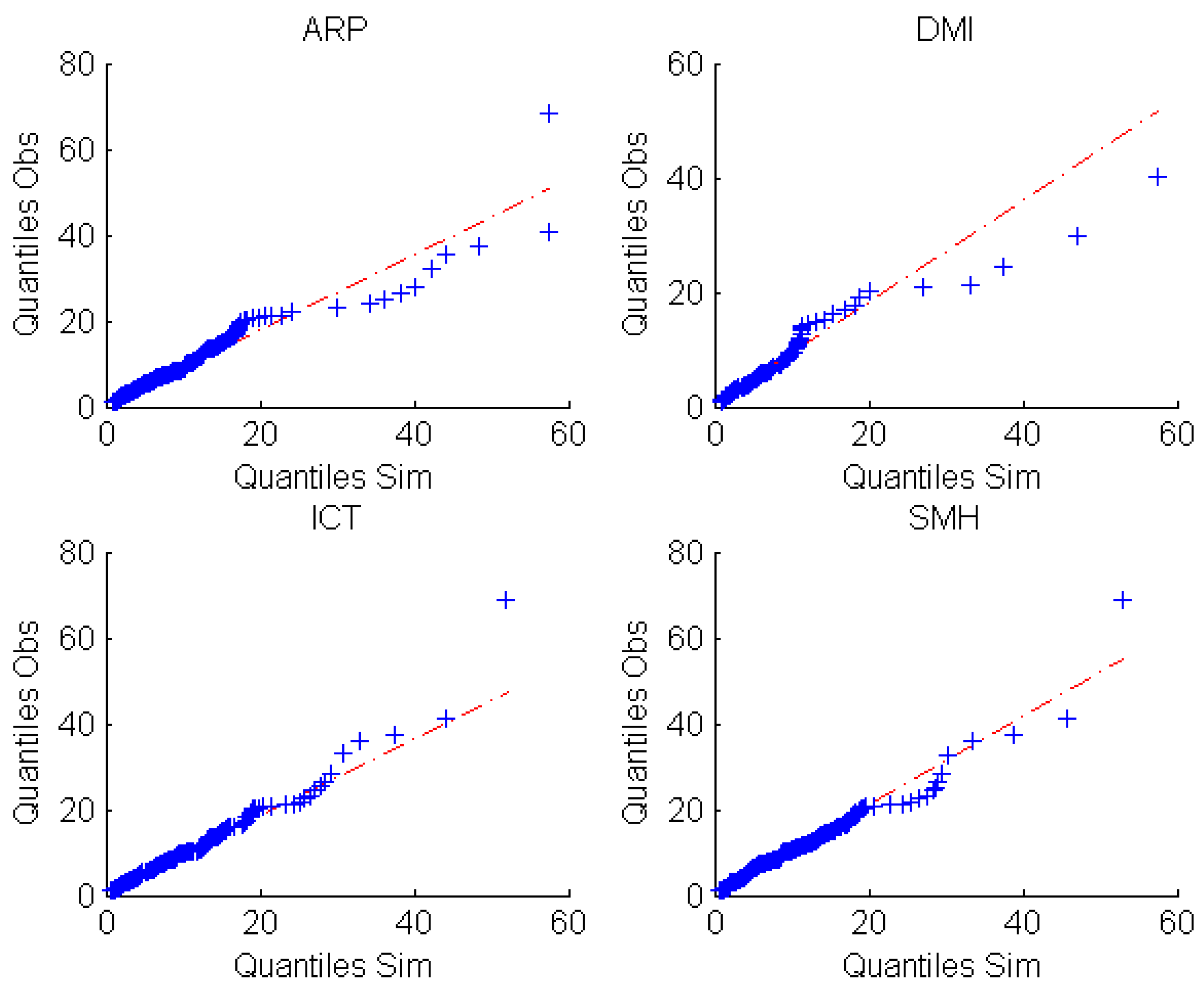
4.3. Evaluation of RCM Simulated Precipitation

Monthly precipitation regimes are shown in Figure 5 for both observed and RCM data. RCM daily rainfall differ from observed rainfall in terms of seasonal distributions (Figure 5). For the dry season months, there is an overestimation of precipitation for all models, except DMI for which there is an underestimation. For the winter months, the monthly totals are underestimated by all models (Figure 5).

Figure 5. Seasonal variability of precipitation (ground data and RCM outputs).

Figure 5. Seasonal variability of precipitation (ground data and RCM outputs).

Simulated rainfall by SMH and ICT is the closest to observed rainfall for the winter months (DJF). Overall, the simulations driven by ECHAM (SMH and ICT) are much closer to the observed cycle than the simulations driven by ARPEGE (ARP and DMI). Moreover, the probability of dry days is underestimated (Table 3), the less accurate results being provided by DMI. As shown in Table 3, DMI has basically no days with zero precipitation: It strongly overestimates the number of wet days. This is may be due to the parametrization of the model or its inability to reproduce precipitation dynamics for the study area. Thus, it is of prime importance to introduce a bias correction to rainfall outputs prior to their use in combination with the hydrological model.

Table 3. Percent of dry days before correction (control period).

Season	Observations	DMI	ICT	SMH	ARP
DJF	44	0	13	22	0.4
MAM	62	0	18	39	0.8
JJA	92	0	43	69	0.3
SON	59	0	17	36	0.2

Table 3. Percent of dry days before correction (control period).

Season	Observations	DMI	ICT	SMH	ARP
DJF	44	0	13	22	0.4
MAM	62	0	18	39	0.8
JJA	92	0	43	69	0.3
SON	59	0	17	36	0.2

This bias correction period is performed using the same calibration period adopted for the hydrological model, 1960–1971 while the validation period for bias correction is 1972–1984.

Figure 6. Scatter plot of precipitation quantiles of bias corrected series including dry day correction and quantiles of observed series for the validation period and MAM spring season.

Figure 6. Scatter plot of precipitation quantiles of bias corrected series including dry day correction and quantiles of observed series for the validation period and MAM spring season.

The method of correction with the fixed threshold at 1 mm has greatly enhanced the comparison for ICT, SMH and ARP. During the validation period, ICT is ranked first to recover the number of dry days for the examined period with only +3% of relative bias on the number of dry days. It is followed by SMH (−7% of relative bias) and then by ARP (+9%). However for DMI, the discrepancy remains large (−58%). The variable thresholds obtained to preserve the number of dry days in the control period are less than 1 mm/d and vary from almost zero to 0.85, depending on the RCM model. For the validation period, a very close performance is obtained for most models either with a fixed threshold of 1 mm/d or with a variable threshold, therefore the first method of a fixed threshold is chosen for the sake of simplicity and to better compare the results between models.

After performing bias correction using the non-parametric quantile-quantile method, the matching between observations and corrected RCM simulations is examined using Kolmogorov-Smirnov and Cramer-von Mises goodness-of-fit tests. The null hypothesis is accepted with both tests for the DJF season for all models. With respect to the MAM season, both tests accept ARP, SMH and ICT simulations and reject the DMI simulation. Q-Q plots are shown in Figure 6. One can see that tests results reflect the good matching between corrected and observed quantiles except for DMI. On the other hand, the null hypothesis is accepted by both tests for only SMH and ICT for the SON season. It is accepted by both tests for SMH, ARP and ICT for summer (JJA).

Figure 7. Comparison of simulated monthly runoff to observed monthly runoff.

Figure 7. Comparison of simulated monthly runoff to observed monthly runoff.

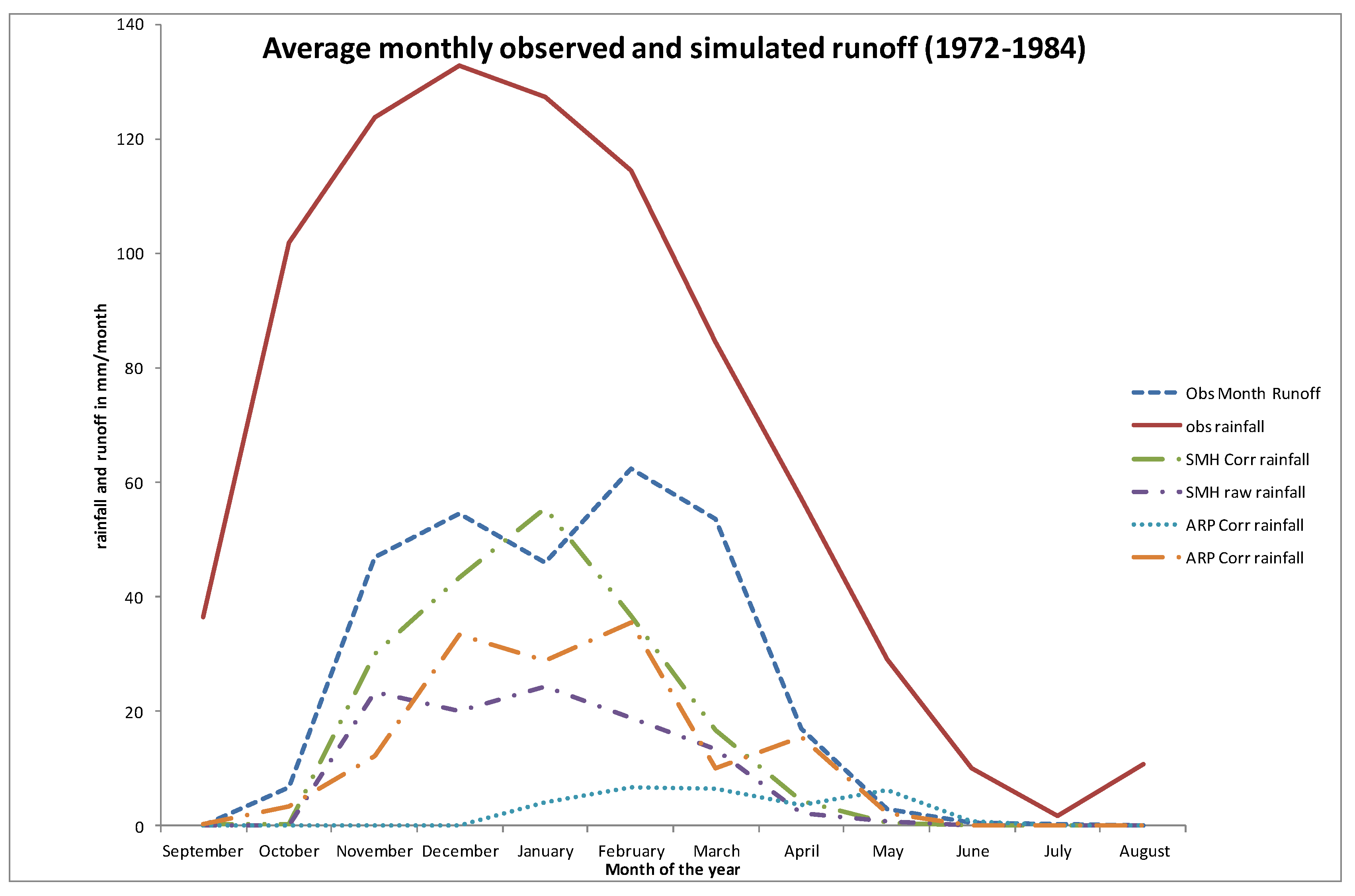
4.4. Hydrological Simulations Driven by Bias-Corrected RCM Precipitation Outputs

In order to examine the hydrological impact of dry day and bias corrections in RCM rainfall series, the calibrated MBBH model is run in two situations: With and without correction of RCM outputs. Average monthly runoff estimations are shown in Figure 7 for SMH and ARP models. The plot suggests that using corrected SMH precipitation, the observed annual regime of runoff is not well reproduced. Indeed, a peak of runoff is simulated for January while there are two peaks in the observed monthly distribution: The most important peak is in February and the second is in December. On the contrary, the corrected precipitation data of ARP reproduces adequately the peaks in runoff for the months of December and February. However, the drawback is that runoff is underestimated for the humid season (from October to March) using ARP corrected precipitation outputs. The mismatch between observed and simulated hydrograph by the bias-corrected outputs of the SMH model is less important than with ARP, except for the timing. Employing a non-corrected rainfall series for SMH, results in biased monthly runoff estimations with two peaks of equal importance in November and January. The use of ARP precipitation series without correction gives rise to an important underestimation of runoff for all months together with an almost uniform hydrograph. Thus, bias correction of precipitation series simulated by the RCMs is absolutely necessary to perform hydrological simulations. It must be noted that bias correction was performed at the daily scale and this does not guarantee an appropriate reduction of bias at the monthly scale. It is worth noting that using the observed precipitation series, the MBBH model tends to underestimate the runoff peak of December while the February peak is well reproduced. As the comparison of RCM bias-corrected precipitation was achieved for the validation period (1972–1984), there is a potential interaction between the hydrological model weakness in validation and the bias correction insufficiencies.

5. Conclusions

The aim of this study was to evaluate RCM outputs in a catchment located in northern Tunisia using a water balance model. The MBBH model was found satisfactory to reproduce runoff at the monthly time scale with stable Nash criterion performance between calibration and validation periods. Since the model only required two parameters to be calibrated using rainfall-runoff data, it is parsimonious. Several RCM precipitation and mean air temperature outputs from the ENSEMBLE projects have been compared to the observed data. For most RCMs, the reproduction of the temperature is acceptable while the precipitation is strongly and systematically biased and requires bias-correction prior to be used in the hydrological model. Therefore, a quantile-quantile bias correction approach was applied to the RCM precipitation intensities together with a drizzle-day correction.

The SMH and ICT RCM models gave rise to the most accurate reproduction of precipitation data after bias correction and a drizzle day correction using a fixed threshold of 1 mm/d. The goodness-of-fit tests accepted the null hypothesis for these models for all seasons. After bias correction, the precipitation amounts in winter season were the most accurately reproduced by the four studied RCMs but the precipitation during the autumn season was the most difficult to reproduce. One explanation could be that in the Mediterranean region during the autumn, rainfall is known to be the most variable in time and space because of the occurrence of convective rainfall events.

With respect to the simulated runoff with the corrected RCM rainfall series, the predicted monthly runoff regime (temporal variability) by ARP reflects the observed regime, where February is the month with the higher runoff values followed by December, which is not the case for SMH results where a single annual peak in January is predicted. Thus, several questions remain unsolved, in particular the effect of correcting rainfall data in the univariate case, while both precipitation and temperature data affects the water balance. To overcome this drawback, Li et al. [33] suggested completing a bivariate approach using a Copula. This could be implemented in further studies on the same catchment.

References

1. Giorgi, F.; Lionello, P. Climate change projections for the Mediterranean region. Glob. Planet. Chang. 2008, 63, 90–104. [Google Scholar] [CrossRef]
2. Majone, B.; Bovolo, C.I.; Bellin, A.; Blenkinsop, S.; Fowler, H.J. Modeling the impacts of future climate change on water resources for the Gallego river basin (Spain). Water Resour. Res. 2012, 48, W01512. [Google Scholar] [CrossRef]
3. Milano, M.; Ruelland, D.; Fernandez, S.; Dezetter, A.; Fabre, J.; Servat, E.; Fritsch, J.-M.; Ardoin-Bardin, S.; Thivet, G. Current state of Mediterranean water resources and future trends under global changes. Hydrolog. Sci. J. 2013, 58, 498–518. [Google Scholar] [CrossRef]
4. Bargaoui, Z.; Tramblay, Y.; Lawin, E.; Servat, E. Seasonal precipitation variability in regional climate simulations over Northern basins of Tunisia. Int. J. Climatol. 2014, 34, 235–248. [Google Scholar] [CrossRef]
5. Fowler, H.J.; Blenkinsop, S.; Tebaldi, C. Linking climate change modelling to impacts studies: Recent advances in downscaling techniques for hydrological modelling. Int. J. Climatol. 2007, 27, 1547–1578. [Google Scholar] [CrossRef]
6. Peel, M.C.; Bloschl, G. Hydrological modelling in a changing world. Prog. Phys. Geogr. 2011, 35, 249–261. [Google Scholar] [CrossRef]
7. Wilby, R.L. Evaluating climate model outputs for hydrological applications. J. Sci. Hydrol. 2010, 55, 1090–1093. [Google Scholar]
8. Maraun, D.; Wetterhall, F.; Ireson, A.M.; Chandler, R.E.; Kendon, E.J.; Widmann, M.; Brienen, S.; Rust, H.W.; Sauter, T.; Themeßl, M.; et al. Precipitation downscaling under climate change: Recent developments to bridge the gap between dynamical models and the end user. Rev. Geophys. 2010, 48. [Google Scholar] [CrossRef]
9. Jacob, D.; Barring, L.; Christensen, O.B.; Christensen, J.H.; de Castro, M.; Deque, M.; Giorgi, F.; Hagemann, S.; Hirschi, M.; Jones, R.; et al. An inter-comparison of regional climate models for Europe: Model performance in present-day climate. Clim. Chang. 2007, 81, 31–52. [Google Scholar]
10. Hagemann, S.; Chen, C.; Haerter, J.O.; Heinke, J.; Gerten, D.; Piani, C. Impact of a statistical bias correction on the projected hydrological changes obtained from three GCMs and two hydrology models. J. Hydrometeorol. 2011, 12, 556–578. [Google Scholar] [CrossRef]
11. Piani, C.; Weedon, G.P.; Best, M.; Gomes, S.M.; Viterbo, P.; Hagemann, S.; Haerter, J.O. Statistical bias correction of global simulated daily precipitation and temperature for the application of hydrological models. J. Hydrol. 2010, 395, 199–215. [Google Scholar] [CrossRef]
12. Piani, C.; Haerter, J.O. Two dimensional bias correction of temperature and precipitation copulas in climate models. Geophys. Res. Lett. 2012, 39. [Google Scholar] [CrossRef]
13. Themeßl, M.; Gobiet, A.; Leuprecht, A. Empirical-statistical downscaling and error correction of daily precipitation from regional climate models. Int. J. Climatol. 2011, 31, 1531–1544. [Google Scholar]
14. Tramblay, Y.; Ruelland, D.; Somot, S.; Bouaicha, R.; Servat, E. High-resolution Med-CORDEX regional climate model simulations for hydrological impact studies: A first evaluation of the ALADIN-Climate model in Morocco. Hydrol. Earth Syst. Sci. 2013, 17, 3721–3739. [Google Scholar] [CrossRef]
15. Kallel, M.R. Dossier Hydrométrique de l’oued Sejnane; Ministry of Agriculture and Water Resources: Tunis, Tunisie, 1980. [Google Scholar]
16. United Nations Environment Programme-World Conservation M. Ichkeul National Park, Tunisia. 2008. Available online: http://www.eoearth.org/view/article/153760/ (accessed on 26 June 2013).
17. Oudin, L.; Hervieu, F.; Michel, C.; Perrin, C.; Andréassian, V.; Anctil, F.; Loumagne, C. Which potential evapotranspiration input for a rainfall-runoff model? Part 2—Towards a simple and efficient PE model for rainfall-runoff modelling. J. Hydrol. 2005, 303, 290–306. [Google Scholar] [CrossRef]
18. Climate Change and Its Impacts: Summary of Research and Results from the ENSEMBLES Project. Available online: http://www.ensembles-eu.org/ (accessed on 26 June 2013).
19. Radu, R.; Déqué, M.; Somot, S. Spectral nudging in a spectral regional climate model. Tellus A 2008, 60, 898–910. [Google Scholar] [CrossRef]
20. Christensen, J.H.; Christensen, O.B.; Lopez, P.; van Meijgaard, E.; Botzet, M. The HIRHAM4 regional atmospheric climate model. DMI Sci. Rep. 1996, 96, 51. [Google Scholar]
21. Giorgi, F.; Mearns, L.O. Introduction to special section: Regional climate modeling revisited. J. Geophys. Res.: Atmos. 1999, 104, 6335–6352. [Google Scholar] [CrossRef]
22. Kjellström, E.; Barring, L.; Gollvik, S.; Hansson, U.; Jones, C.; Samuelsson, P.; Rummukainen, M.; Ullersig, A.; Willen, U.; Wyser, K. A 140-year Simulation of European Climate with the New Version of the Rossby Centre Regional Atmospheric Climate Model (RCA3); SMHI: Norrkoping, Sweden.
23. Kobayashi, T.; Matsuda, S.; Nagai, H.; Teshima, J. A bucket with a bottom hole (BBH) model of soil hydrology. In Soil-Vegetation-Atmosphere Transfer Schemes and Large-Scale Hydrological Models; Dolman, A.J., Hall, A.J., Kavvas, M.L., Oki, T., Pomeroy, J.W., Eds.; IAHS Press: Wallingford, UK, 2001; pp. 41–75. [Google Scholar]
24. Bargaoui, Z.; Houcine, A. Sensitivity to calibration data of simulated soil moisture related drought indices. Rev. Sécher. 2010, 21, 294–300. [Google Scholar]
25. Cosby, B.J.; Hornberger, G.M.; Clapp, R.B.; Ginn, T.R. A statistical exploration of the relationships of soil moisture characteristics to the physical properties of soils. Water Resour. Res. 1984, 20, 682–690. [Google Scholar] [CrossRef]
26. Eagleson, P.S. Climate, soil, and vegetation 6. Dynamics of the annual water balance. Water Resour. Res. 1978, 14, 749–764. [Google Scholar] [CrossRef]
27. Eagleson, P.S. The evolution of modern hydrology (from watershed to continent in 30 years). Adv. Water Resour. 1994, 17, 3–18. [Google Scholar] [CrossRef]
28. Darling, D.A. The Kolmogorov-Smirnov, Cramér-von Mises tests. Ann. Math. Stat. 1957, 28, 823–838. [Google Scholar] [CrossRef]
29. Déqué, M. Frequency of precipitation and temperature extremes over France in an anthropogenic scenario: Model results and statistical correction according to observed values. Glob. Planet. Chang. 2007, 57, 16–26. [Google Scholar] [CrossRef]
30. Michelangeli, P.A.; Vrac, M.; Loukos, H. Probabilistic downscaling approaches: Application to wind cumulative distribution functions. Geophys. Res. Lett. 2009, 36, L11708. [Google Scholar] [CrossRef]
31. Vrac, M.; Drobinski, P.; Merlo, A.; Herrmann, M.; Lavaysse, C.; Li, L.; Somot, S. Dynamical and statistical downscaling of the French Mediterranean climate: Uncertainty assessment. Nat. Hazards Earth Syst. Sci. 2012, 12, 2769–2784. [Google Scholar] [CrossRef] [Green Version]
32. Lavaysse, C.; Vrac, M.; Drobinski, P.; Lengaigne, M.; Vischel, T. Statistical downscaling of the French Mediterranean climate: Assessment for present and projection in an anthropogenic scenario. Nat. Hazards Earth Syst. Sci. 2012, 12, 651–670. [Google Scholar] [CrossRef] [Green Version]
33. Li, C.; Sinha, E.; Horton, D.E.; Diffenbaugh, N.S.; Michalak, A.M. Joint bias correction of temperature and precipitation in climate model simulations. J. Geophys. Res. Atmos. 2014. [Google Scholar] [CrossRef]