
Detailed Urban Heat Island Projections for Cities Worldwide: Dynamical Downscaling CMIP5 Global Climate Models

Abstract
:1. Introduction
2. Numerical Model, Experiment Setup and Model Evaluation
2.1. The UrbClim Model
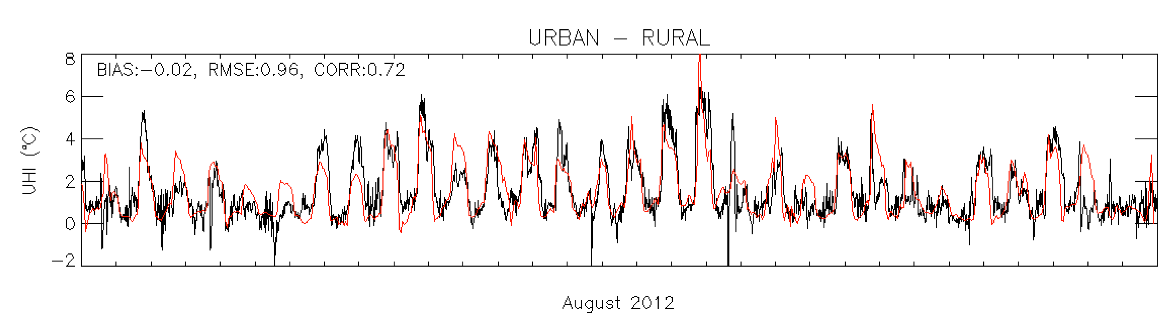
2.2. Model Evaluation

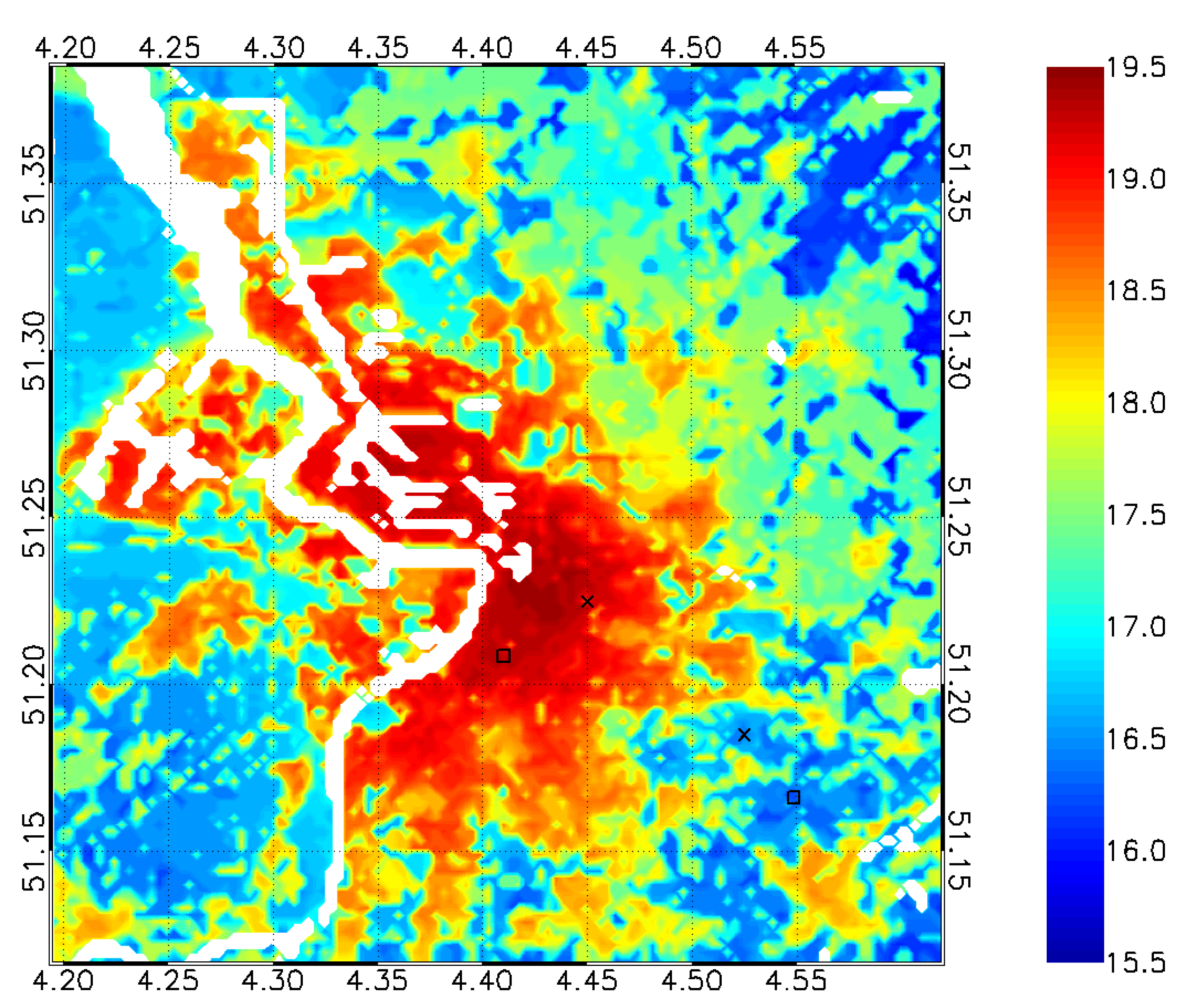
2.3. UHI Indicator Definition

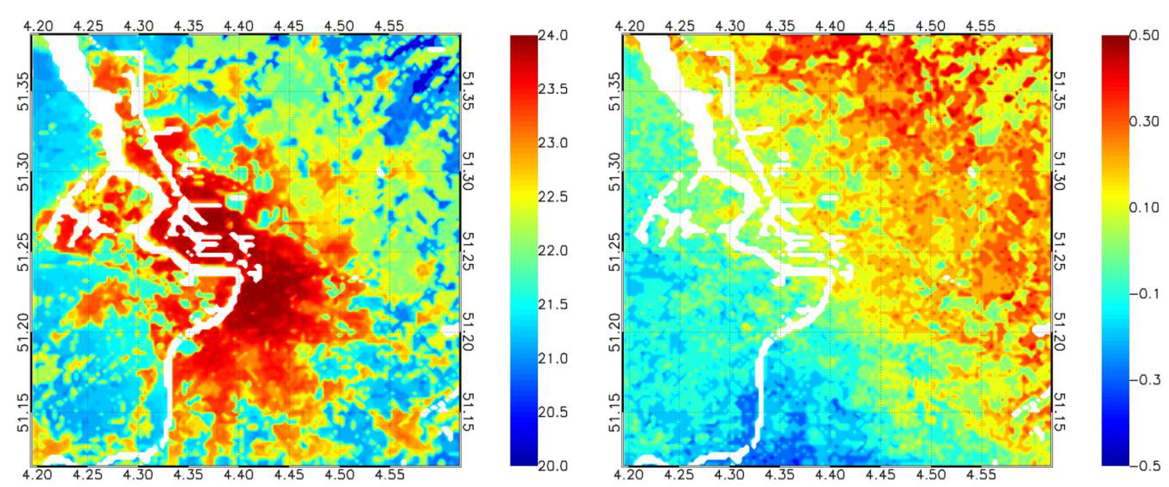
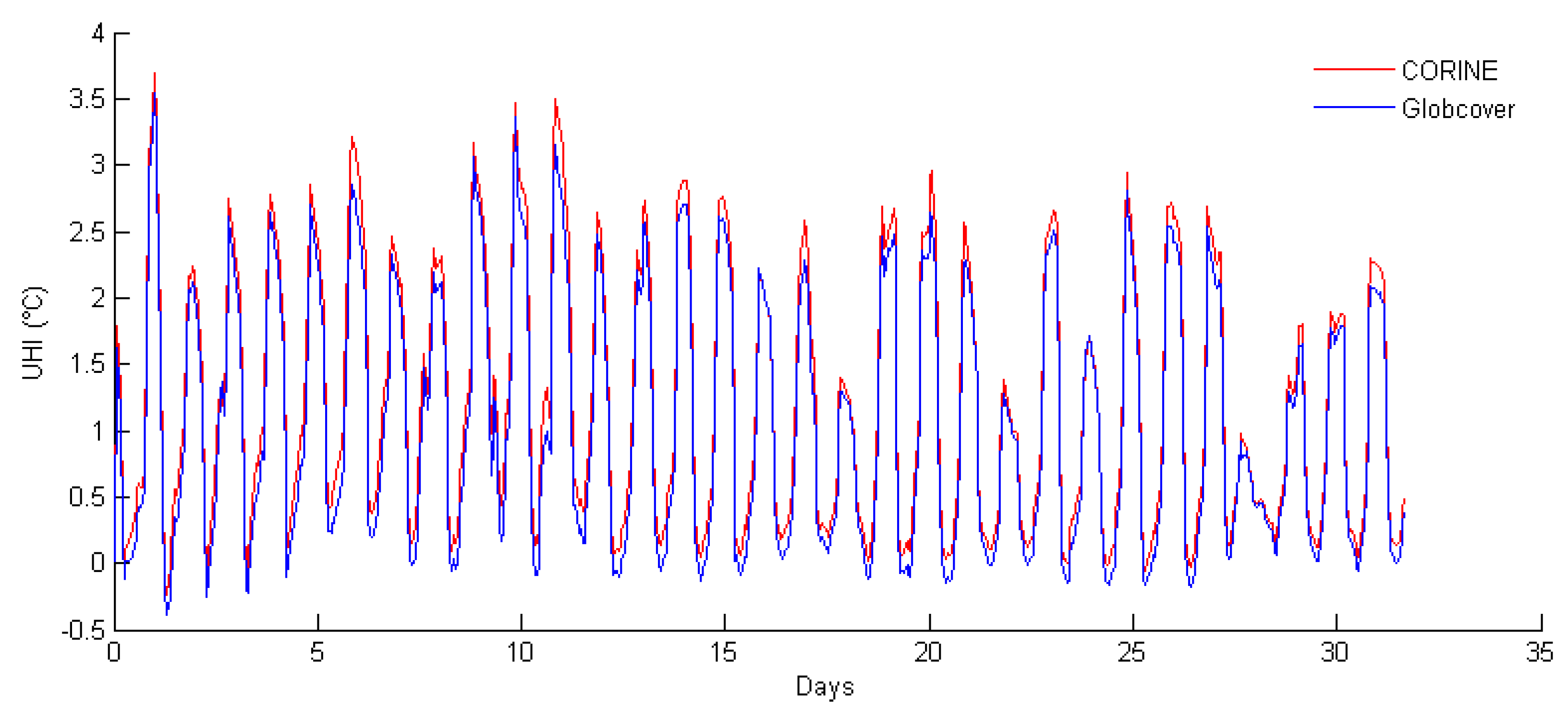
2.4. Towards the Global Applicability of the UrbClim Model

| City | Country | Latitude (°) | Longitude (°) | Domain Size (km2) | Model Resolution | Summer Period |
|---|---|---|---|---|---|---|
| Almada | Portugal | 38.68 | 9.16 | 30 × 30 | 250 m | June–August |
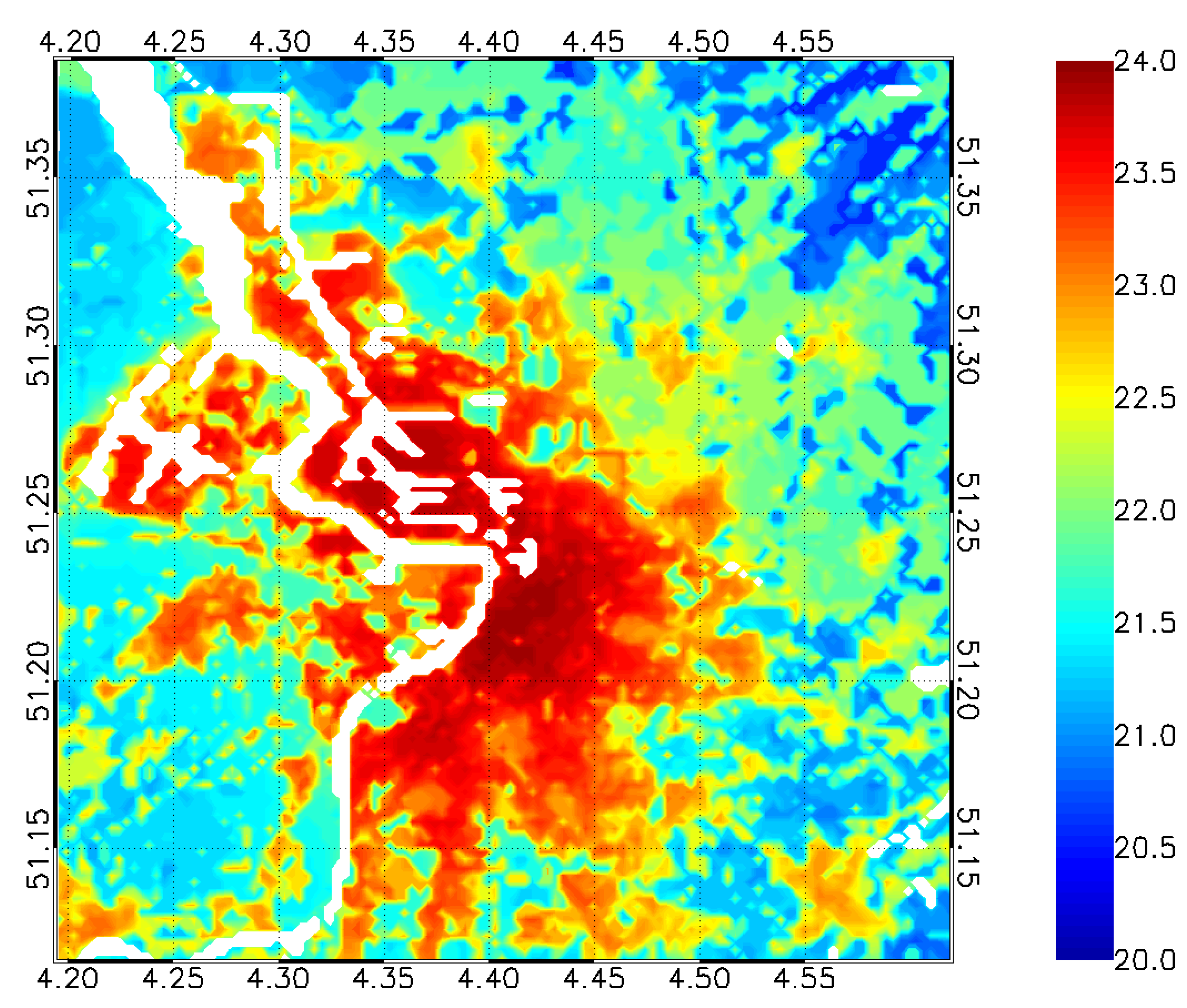
| Antwerp | Belgium | 51.25 | 4.41 | 30 × 30 | 250 m | June–August |
| Berlin | Germany | 52.52 | 13.38 | 50 × 50 | 250 m | June–August |
| Bilbao | Spain | 43.26 | −2.92 | 30 × 30 | 250 m | June–August |
| London | U.K. | 51.51 | −0.13 | 90 × 90 | 500 m | June–August |
| New York | USA | 40.71 | −74.01 | 120 × 120 | 1 km | June–August |
| Rio de Janeiro | Brazil | −22.84 | −43.32 | 70 × 70 | 500 m | January–March |
| Skopje | Macedonia | 42.00 | 21.43 | 30 × 30 | 250 m | June–August |
3. Coupling to GCM Output Fields
3.1. Input from the GCMs for Climate Projections
| Category | Variable | Required Time Increment |
|---|---|---|
| Surface | Downwelling short-wave radiation | 3 h |
| Downwelling long-wave radiation | 3 h | |
| Surface air pressure | 3 h | |
| Air temperature at surface | 3 h | |
| U component of wind velocity at surface | 3 h | |
| V component of wind velocity at surface | 3 h | |
| Specific humidity at surface | 3 h | |
| Sea | Sea surface temperature | monthly |
| Precipitation | Total precipitation | 3 h |
| Convective precipitation | 3 h | |
| Vertical profiles | U component of wind velocity | 6 h |
| V component of wind velocity | 6 h | |
| Temperature profile | 6 h | |
| Specific humidity profile | 6 h | |
| Soil | Soil temperature | monthly |
| Soil moisture content | monthly |
| Model | Institute | ΔLon (°) | ΔLat (°) |
|---|---|---|---|
| ACCESS1.0 | CSIRO/BOM | 1.875 | 1.25 |
| BNU_ESM | BNU | 2.8125 | 2.79 |
| CCSM4 | NCAR | 1.25 | 0.94 |
| CNRM_CM5 | CNRM | 1.40625 | 1.4 |
| FGOALS-G2 | CAS | 2.8125 | 2.79 |
| GFDL-ESM2M | GFDL | 2.5 | 2.02 |
| GISS-E2-R | NASA | 2.5 | 2 |
| HadGem2-ES | MOHC | 1.875 | 1.25 |
| IPSL-CM5A-MR | IPSL | 2.5 | 1.2676 |
| MIROC-ESM-CHEM | Univ. Tokyo | 2.8125 | 2.79 |
| MRI-CGCM3 | MRI | 1.125 | 1.1121 |
3.2. Construction of Vertical Profiles


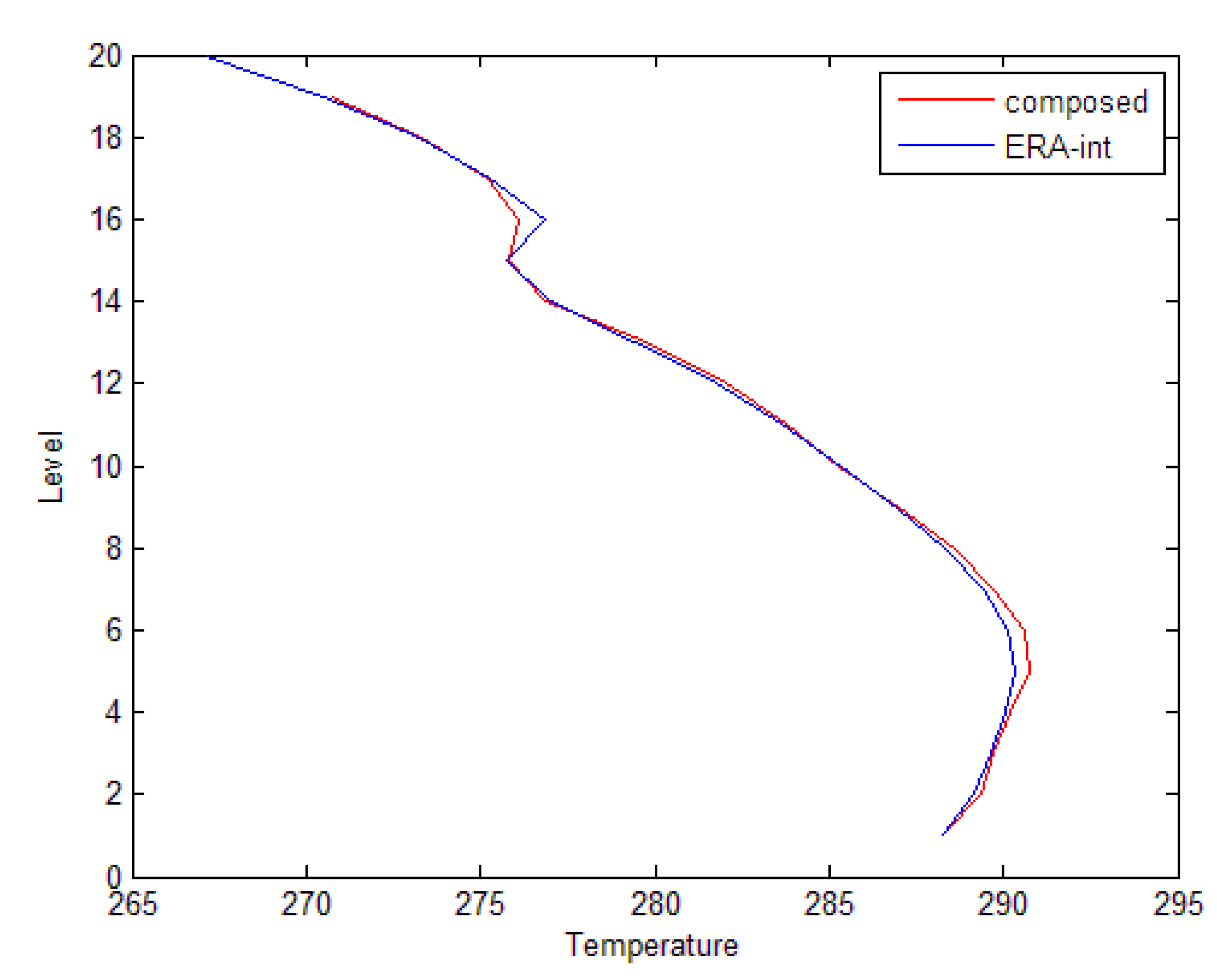
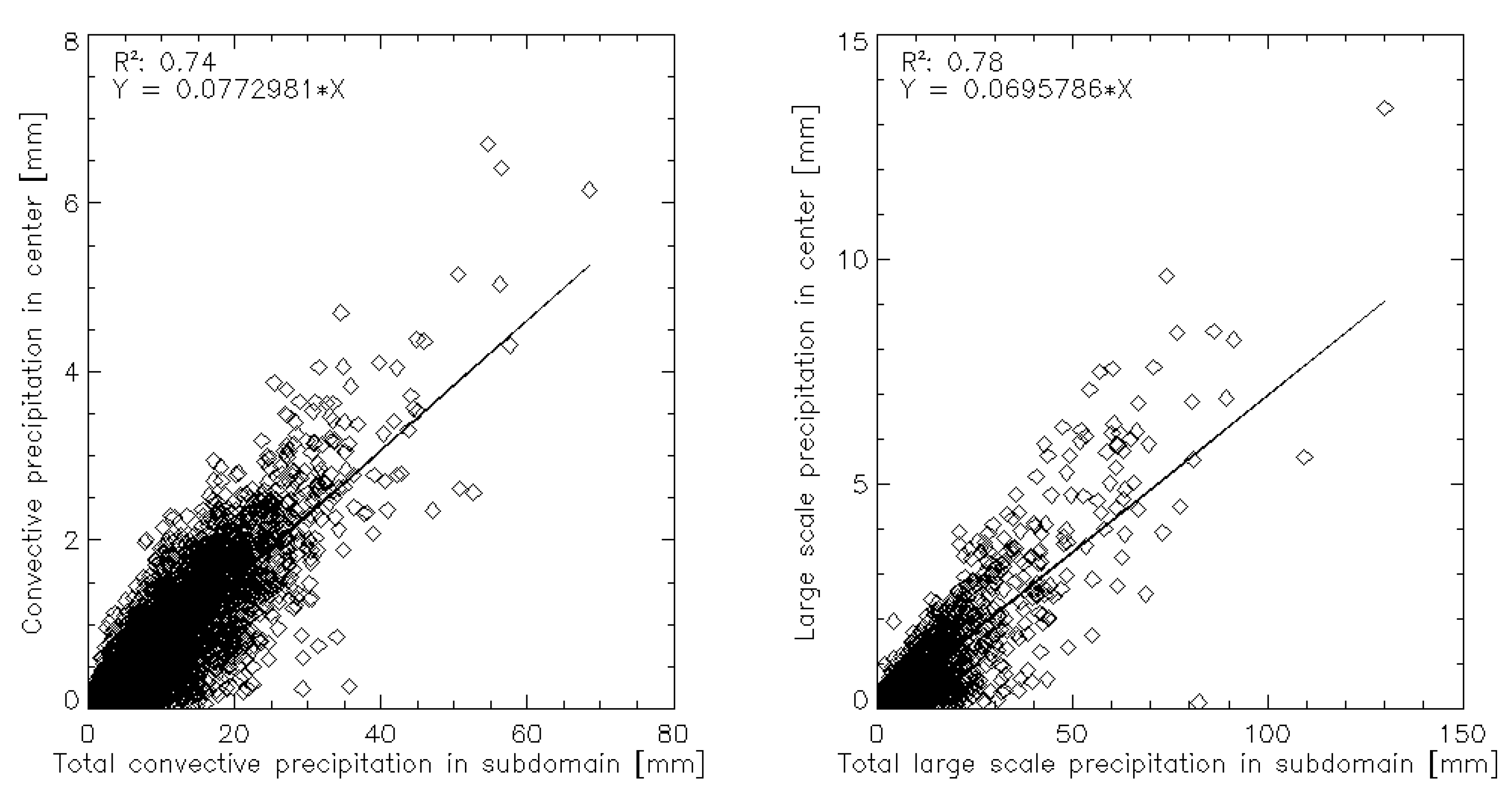
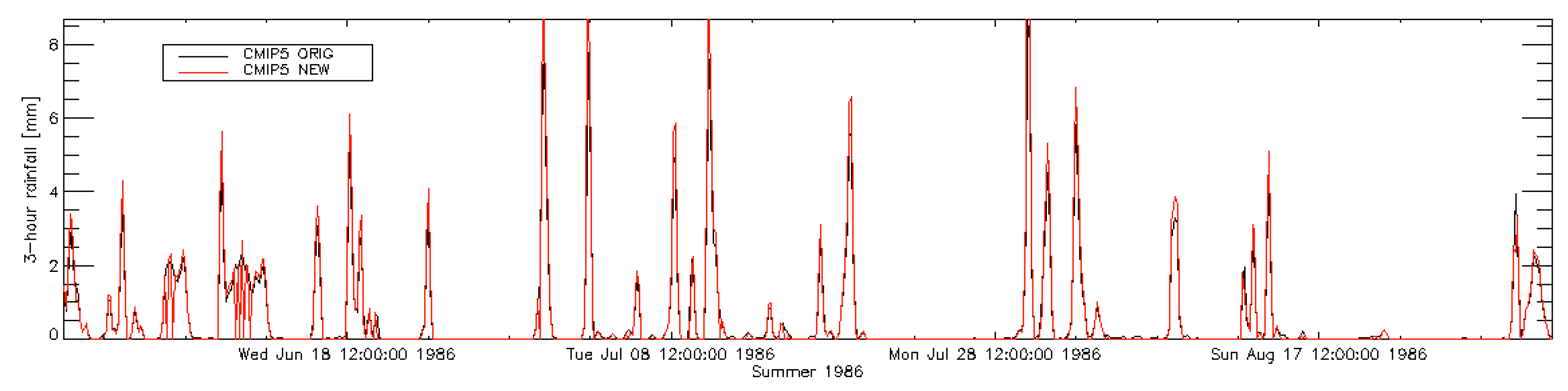
3.3. Precipitation Downscaling

3.4. Bias Correction
| Almada | Antwerp | Berlin | Bilbao | London | New York | Rio | Skopje | |
|---|---|---|---|---|---|---|---|---|
| ACCESS1.0 | −1.1 | −1.9 | −2.0 | +2.8 | −2.2 | −0.1 | +1.3 | −1.5 |
| BNU_ESM | −6.4 | −2.2 | −1.7 | −2.4 | −4.1 | −3.1 | +1.5 | −3.5 |
| CCSM4 | −2.4 | −0.5 | −1.2 | +1.3 | −0.9 | −1.0 | +0.5 | −0.9 |
| CNRM_CM5 | −0.9 | −2.2 | −3.9 | +1.1 | −3.5 | −1.3 | −0.7 | +0.1 |
| FGOALS-G2 | +0.8 | +1.2 | −0.6 | +4.0 | +0.1 | +2.4 | +3.0 | +0.2 |
| GFDL-ESM2M | −4.2 | +1.2 | +0.5 | +1.0 | +1.2 | +0.8 | −0.8 | −0.3 |
| GISS-E2-R | −2.1 | +0.7 | +0.6 | +1.8 | −0.1 | +1.9 | −0.9 | +3.6 |
| HadGem2-ES | −0.1 | −2.8 | −4.2 | +3.4 | −2.9 | −1.3 | −0.1 | −1.4 |
| IPSL-CM5A-MR | +1.2 | −1.5 | −0.9 | −0.8 | −2.4 | −0.5 | +0.3 | +1.5 |
| MIROC-ESM-CHEM | −3.1 | −1.3 | −1.9 | +1.4 | −1.3 | −3.4 | +2.1 | +0.4 |
| MRI-CGCM3 | −0.5 | +0.9 | +1.1 | +2.8 | +1.0 | +2.3 | +1.0 | +3.3 |
4. Results and Discussion
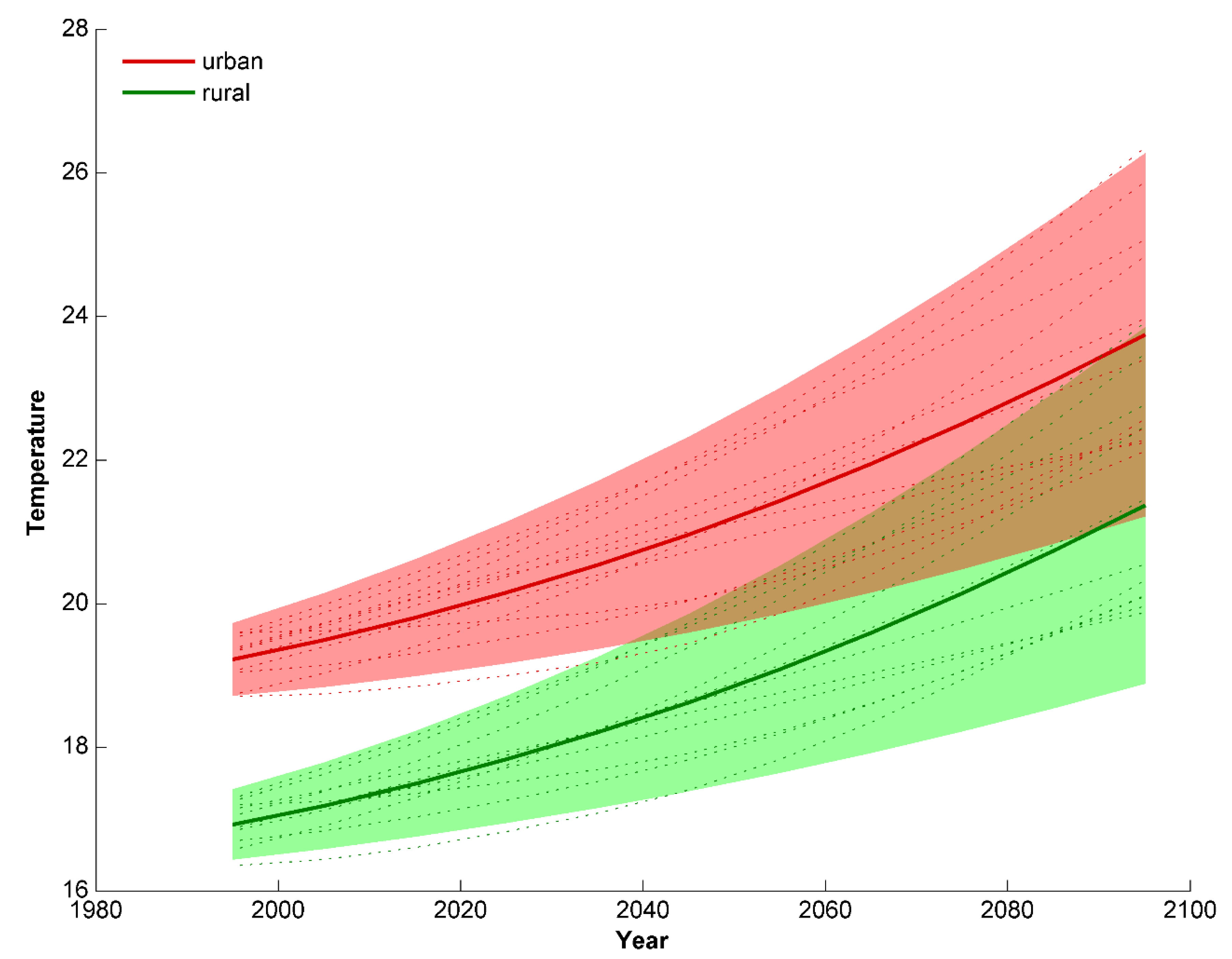
4.1. UHI Projection Results

| City | Ref. UHI (°C) | ΔRural (°C) | ΔUrban (°C) | ΔUHI (°C) | Uncertainty (°C) |
|---|---|---|---|---|---|
| Almada | 2.47 | 4.51 | 4.58 | 0.07 | 0.07 |
| Antwerp | 2.30 | 4.12 | 4.20 | 0.08 | 0.07 |
| Berlin | 2.70 | 4.53 | 4.64 | 0.11 | 0.09 |
| Bilbao | 2.12 | 4.56 | 4.63 | 0.08 | 0.06 |
| London | 2.98 | 4.31 | 4.32 | 0.01 | 0.08 |
| New York | 3.57 | 4.87 | 5.08 | 0.21 | 0.12 |
| Rio | 2.95 | 3.30 | 3.18 | -0.12 | 0.10 |
| Skopje | 2.25 | 6.74 | 6.85 | 0.10 | 0.09 |
4.2. Discussion Regarding the UHI Intensity Changes
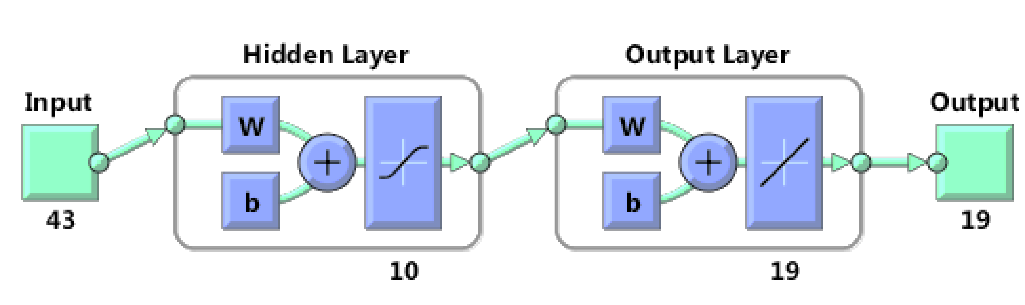
4.3. Applying a Statistical Method

5. Conclusions
Acknowledgments
Author Contributions
Conflicts of Interest
References
- Meehl, G.A.; Tebaldi, C. More intense, more frequent, and longer lasting heat waves in the 21st century. Science 2004, 13, 994–997. [Google Scholar] [CrossRef] [PubMed]
- Diffenbaugh, N.S.; Giorgi, F. Climate change hotspots in the CMIP5 global climate model ensemble. Clim. Chang. 2012, 114, 813–822. [Google Scholar] [CrossRef] [PubMed]
- Schär, C.; Vidale, P.L.; Luthi, D.; Frei, C.; Haberli, C.; Liniger, M.A.; Appenzeller, C. The role of increasing temperature variability in European summer heat waves. Nature 2004, 427, 332–336. [Google Scholar] [CrossRef] [PubMed]
- Oke, T.R. Urban climates and global environmental change. In Applied Climatology: Principles and Practice; Routledge: New York, NY, USA, 1997; pp. 273–287. [Google Scholar]
- Fischer, E.M.; Oleson, K.W.; Lawrence, D.M. Contrasting urban and rural heat stress responses to climate change. Geophys. Res. Lett. 2012, 39, L03705. [Google Scholar] [CrossRef]
- Oleson, K. Contrasts between urban and rural climate in CCSM4 CMIP5 climate change scenarios. Journal of Climate 2012, 25, 1390–1412. [Google Scholar] [CrossRef]
- Hamdi, R.; van de Vyver, H.; de Troch, R.; Termonia, P. Assessment of three dynamical urban climate downscaling methods: Brussels’s future urban heat island under an A1B emission scenario. Int. J. Climatol. 2014, 34, 978–999. [Google Scholar] [CrossRef]
- McCarthy, M.P.; Harpham, C.; Goodess, C.M.; Jones, P.D. Simulating climate change in UK cities using a regional climate model, HadRM3. Int. J. Climatol. 2012, 32, 1875–1888. [Google Scholar] [CrossRef]
- Kusaka, H.; Hara, M.; Takane, Y. Urban climate projection bythe WRF model at 3-km horizontal grid increment: Dynamicaldownscaling and predicting heat stress in the 2070’s August for Tokyo, Osaka, and Nagoya metropolises. J. Meteorol. Soc. Jpn. 2012, 90B, 47–63. [Google Scholar] [CrossRef]
- Argüeso, D.; Evans, J.P.; Fita, L.; Bormann, K.J. Temperature response to future urbanization and climate change. Clim. Dyn. 2014, 42, 2183–2199. [Google Scholar] [CrossRef]
- Lemonsu, A.; Kounkou-Arnaud, R.; Desplat, J.; Salagnac, J.L.; Masson, V. Evolution of the Parisian urban climate under a global changing climate. Clim. Chang. 2013, 116, 679–692. [Google Scholar] [CrossRef]
- IPCC. Climate Change 2013: The Physical Science Basis; Cambridge University Press: Cambridge, UK; New York, NY, USA, 2013. [Google Scholar]
- De Ridder, K.; Lauwaet, D.; Maiheu, B. UrbClim—A fast urban boundary layer climate model. Urban Clim. 2015, 12, 21–48. [Google Scholar] [CrossRef]
- De Ridder, K.; Schayes, G. The IAGL land surface model. J. Appl. Meteorol. 1997, 36, 167–182. [Google Scholar] [CrossRef]
- Kanda, M.; Kanega, M.; Kawai, T.; Moriwaki, R.; Sugawara, H. Roughness lengths for momentum and heat derived from outdoor urban-scale models. J. Appl. Meteorol. Climatol. 2007, 46, 1067–1079. [Google Scholar] [CrossRef]
- De Ridder, K.; Bertrand, C.; Casanova, G.; Lefebvre, W. Exploring a new method for the retrieval of urban thermophysical properties using thermal infrared remote sensing and deterministic modelling. J. Geophys. Res. 2012, 117, JD017194. [Google Scholar]
- Ikeda, R.; Kusaka, H. Proposing the simplification of the multilayer urban canopy model: Intercomparison study of four models. J. Appl. Meteorol. Climatol. 2010, 49, 902–919. [Google Scholar] [CrossRef]
- Masson, V. A physically-based scheme for the urban energy budget in atmospheric models. Bound.-Layer Meteorol. 2000, 94, 357–397. [Google Scholar] [CrossRef]
- Oleson, K.W.; Bonan, G.B.; Feddema, J.; Vertenstein, M.; Grimmond, C.S.B. An urban parameterization for a global climate model. 1. Formulation and evaluation for two cities. J. Applied Meteorol. Climatol. 2008, 47, 1038–1060. [Google Scholar]
- Jürges, W. Die Wärmeübergang an einer ebenen Wand. Beih. Gesundh. Ing. 1924, 19, 1227–1249. [Google Scholar]
- Rowley, F.B.; Algren, A.B.; Blackshaw, J.L. Surface conductances as affected by air velocity, temperature, and character of surface. ASHRAE Trans. 1930, 36, 429–446. [Google Scholar]
- De Ridder, K. Testing Brutsaert’s temperature roughness parameterization for representing urban surfaces in atmospheric models. Geophys. Res. Lett. 2006, 33, GL026572. [Google Scholar] [CrossRef]
- De Ridder, K.; Lefebre, F.; Adriaensen, S.; Arnold, U.; Beckroege, W.; Bronner, C.; Damsgaard, O.; Dostal, I.; Dufek, J.; Hirsch, J.; et al. Simulating the impact of urban sprawl on air quality and population exposure in the German Ruhr area. Part I: Reproducing the base state. Atmos. Environ. 2008, 42, 7059–7069. [Google Scholar] [CrossRef]
- Nakamura, Y.; Oke, T.R. Wind, temperature and stability conditions in an E-W oriented urban canyon. Atmos. Environ. 1988, 22, 2691–2700. [Google Scholar] [CrossRef]
- Erell, E.; Williamson, T. Simulating air temperature in an urban street canyon in all weather conditions using measured data at a reference meteorological station. Int. J. Climatol. 2006, 26, 1671–1694. [Google Scholar] [CrossRef]
- Danielson, J.J.; Gesch, D.B. Global Multi-Resolution Terrain Elevation Data 2010 (GMTED2010): U.S. Geological Survey Open-File Report 2011–1073; U.S. Geological Survey: Reston, VA, USA.
- European Commission. CORINE Land Cover Technical Guide; European Commission Publications: Rue Mercier, Luxembourg, 2013; p. 35. [Google Scholar]
- Gutman, G.; Ignatov, A. Derivation of green vegetation fraction from NOAA/AVHRR for use in weather prediction models. Int. J. Remote Sens. 1998, 19, 1533–1543. [Google Scholar]
- Piringer, M.; Joffre, S.; Baklanov, A.; Christen, A.; Deserti, M.; de Ridder, K.; Emeis, S.; Mestayer, P.; Tombrou, M.; Middleton, D.; et al. The surface energy balance and the mixing height in urban areas—Activities and recommendations of COST Action 715. Bound.-Layer Meteorol. 2007, 124, 3–24. [Google Scholar] [CrossRef]
- Oke, T.R. Boundary Layer Climates; Taylor & Francis: New York, NY, USA, 2002; p. 464. [Google Scholar]
- Pielke, R.A., Sr. Mesoscale Meteorological Modelling, 2nd ed.; Academic Press: San Diego, CA, USA, 2002; p. 676. [Google Scholar]
- Wouters, H.; Demuzere, M.; de Ridder, K.; van Lipzig, N.P.M.; Vogel, G. Exploring water-storage and evaporation for urban impervious land cover. Urban Clim. 2015. submitted. [Google Scholar]
- Garratt, J.R. The Atmospheric Boundary Layer; Cambridge University Press: Cambridge, UK, 1992; p. 316. [Google Scholar]
- Best, M.J.; Grimmond, C.S.B. Analysis of the seasonal cycle within the first international urban land-surface model comparison. Bound. Layer Meteorol. 2013, 146, 421–446. [Google Scholar] [CrossRef]
- Bohnenstengel, S.I.; Evans, S.; Clark, P.A.; Belcher, S.E. Simulations of the London urban heat island. Q. J. R. Meteorol. Soc. 2011, 137, 1625–1640. [Google Scholar] [CrossRef]
- Salamanca, F.; Martilli, A.; Tewari, M.; Chen, F. A study of the urban boundary layer using different urban parameterizations and high-resolution urban canopy parameters with WRF. J. Appl. Meteorol. Climatol. 2011, 50, 1107–1128. [Google Scholar] [CrossRef]
- Chemel, C.; Sokhi, R.S. Response of London’s urban heat island to a marine air intrusion in an easterly wind regime. Bound.-Layer Meteorol. 2012, 144, 65–81. [Google Scholar] [CrossRef] [Green Version]
- Loridan, T.; Lindberg, F.; Jorba, O.; Kotthaus, S.; Grossman-Clarke, S.; Grimmond, C.S.B. High resolution simulation of the variability of surface energy balance fluxes across central London with urban zones for energy partitioning. Bound. Layer Meteorol. 2013, 147, 493–523. [Google Scholar] [CrossRef]
- Lauwaet, D.; de Ridder, K.; Saeed, S.; Brisson, E.; van Lipzig, N.P.M.; Maiheu, B.; Hooyberghs, H. Assessing the current and future urban heat island of Brussels. Urban Clim. 2015. under review. [Google Scholar]
- Reconciling Adaptation, Mitigation and Sustainable Development for Cities (RAMSES). Available online: http://www.ramses-cities.eu (accessed on 17 March 2015).
- North Atlantic Climate (NACLIM). Available online: http://www.naclim.eu (accessed on 17 March 2015).
- Bontemps, S. GLOBCOVER 2009: Products Description and Validation Report; European Space Agency: Frascati, Italy, 2009. [Google Scholar]
- Li, D.; Bou-Zeid, E. Synergistic interactions between urban heat islands and heat waves: The impact in cities Is larger than the sum of its parts. J. Appl. Meteorol. Climatol. 2013, 52, 2051–2064. [Google Scholar] [CrossRef]
- Oleson, K.W.; Bonan, G.B.; Feddema, J.; Jackson, T. An examination of urban heat island characteristics in a global climate model. Int. J. Climatol. 2011, 31, 1848–1865. [Google Scholar] [CrossRef]
© 2015 by the authors; licensee MDPI, Basel, Switzerland. This article is an open access article distributed under the terms and conditions of the Creative Commons Attribution license (http://creativecommons.org/licenses/by/4.0/).
Share and Cite
Lauwaet, D.; Hooyberghs, H.; Maiheu, B.; Lefebvre, W.; Driesen, G.; Van Looy, S.; De Ridder, K. Detailed Urban Heat Island Projections for Cities Worldwide: Dynamical Downscaling CMIP5 Global Climate Models. Climate 2015, 3, 391-415. https://doi.org/10.3390/cli3020391
Lauwaet D, Hooyberghs H, Maiheu B, Lefebvre W, Driesen G, Van Looy S, De Ridder K. Detailed Urban Heat Island Projections for Cities Worldwide: Dynamical Downscaling CMIP5 Global Climate Models. Climate. 2015; 3(2):391-415. https://doi.org/10.3390/cli3020391
Chicago/Turabian StyleLauwaet, Dirk, Hans Hooyberghs, Bino Maiheu, Wouter Lefebvre, Guy Driesen, Stijn Van Looy, and Koen De Ridder. 2015. "Detailed Urban Heat Island Projections for Cities Worldwide: Dynamical Downscaling CMIP5 Global Climate Models" Climate 3, no. 2: 391-415. https://doi.org/10.3390/cli3020391