Article

The Effect of Land Cover/Land Use Changes on the Regional Climate of the USA High Plains

1
Geography Department, University of Nevada, Reno, NV 89557, USA
2
School of Natural Resources and Department of Civil Engineering, University of Nebraska-Lincoln, 311 Hardin Hall, Lincoln, NE 68583, USA
3
Department of Biological Systems Engineering, University of Nebraska-Lincoln, 239 L.W. Chase Hall, Lincoln, NE 68583, USA
*
Author to whom correspondence should be addressed.
Climate 2014, 2(3), 153-167; https://doi.org/10.3390/cli2030153
Submission received: 26 June 2014 / Revised: 1 August 2014 / Accepted: 5 August 2014 / Published: 11 August 2014
(This article belongs to the Special Issue Land-Use/Cover Change Impacts on Climate)

Abstract

:
We present the detection of the signatures of land use/land cover (LULC) changes on the regional climate of the US High Plains. We used the normalized difference vegetation index (NDVI) as a proxy of LULC changes and atmospheric CO2 concentrations as a proxy of greenhouse gases. An enhanced signal processing procedure was developed to detect the signatures of LULC changes by integrating autoregression and moving average (ARMA) modeling and optimal fingerprinting technique. The results, which are representative of the average spatial signatures of climate response to LULC change forcing on the regional climate of the High Plains during the 26 years of the study period (1981–2006), show a significant cooling effect on the regional temperatures during the summer season. The cooling effect was attributed to probable evaporative cooling originating from the increasing extensive irrigation in the region. The external forcing of atmospheric CO2 was included in the study to suppress the radiative warming effect of greenhouse gases, thus, enhancing the LULC change signal. The results show that the greenhouse gas radiative warming effect in the region is significant, but weak, compared to the LULC change signal. The study demonstrates the regional climatic impact of anthropogenic induced atmospheric-biosphere interaction attributed to LULC change, which is an additional and important climate forcing in addition to greenhouse gas radiative forcing in High Plains region.

1. Introduction

Extensive land use/land cover changes (LULC) and their climate forcing represent an important human influence on atmospheric temperature trends [1]. Several studies using both modeled and observed data have documented the perturbation and impacts of LULC changes on climate (e.g., [2,3,4,5,6,7,8,9,10,11,12]). Authors in [1] expressed the importance of detecting LULC changes accurately at appropriate scales as so to better understand their impacts on climate and provide improved prediction of future climate. In this study, we attempt to detect the signature of the external forcing of LULC change on the regional climate of the High Plains. The proxy investigated for the forcing on the regional climate due to LULC change is the Normalized Difference Vegetation Index (NDVI). The index has been widely used to study and monitor vegetation coverage, change, and development in several ecosystems. On a daily basis, vegetation as a component of the biosphere interacts with the atmosphere through its direct influence on the partitioning between latent and sensible heat fluxes [13,14]. In addition to LULC change, we included atmospheric carbon dioxide (CO2) concentrations as a proxy of greenhouse gas forcing on climate. The increase in atmospheric CO2 concentration has been used in several studies to express the net radiative forcing contribution of anthropogenic greenhouse gases on climate [15].
For the detection of an external forcing signal on climate, Authors in [16] proposed a rationale of developing filters that optimized external forcing signal to natural climate noise ratio. The filters function as projectors of the forced climate signals from a dimensional space of high noise to a low noise dimensional space. The dimensional space in this study is represented by the two-dimensional signals; LULC change and greenhouse radiative warming. This technique referred to as optimal fingerprinting is a space and time dependent analysis. The climate response consists of a time series of observed climate indices from which the anticipated external forcing signal can most readily be distinguished from natural climate noise (also referred to as natural climate variability). Results from climate models indicate that temperature and atmospheric moisture content are good indices [17,18,19]. This is because temperature is a smooth field with relatively little variability, and atmospheric moisture is a first order function to temperature that shares much of the smoothness. Authors in [20] showed that the signal to noise ratio was comparably higher in near-surface temperature than in any other indices. In addition, temperature has been observed for a comparatively long time, providing reasonably good information on the time dependence of observed climate variability. Therefore in this study we investigated temperature as the observed climate response variable.
The intrinsic time dependence of climate variables is a confounding factor in the optimal fingerprinting technique, explicitly, in determining the covariance matrix. Authors in [21,22] suggested the method of reducing the complexity of the covariance structure by representing the natural climate variability as a superposition of a finite number of principal oscillation patterns. The basic idea is to introduce an auto-regression moving average (ARMA) type of dynamic modeling approach into the time domain. In this study, we used this approach by applying the linear transformation of ARMA pre-filters to identify and suppress time dependence/autocorrelation in the analysis. With the assumption that natural climate variability is a stationary process, ARMA pre-filters were fit to generate near-stationary residuals, which represent natural climate variability (noise). By introducing the ARMA pre-filters, our study developed an enhanced signal processing procedure that maximized the signal to noise ratio to detect the signal of LULC change on observed temperatures in the High Plains.

2. Methodology and Analyses

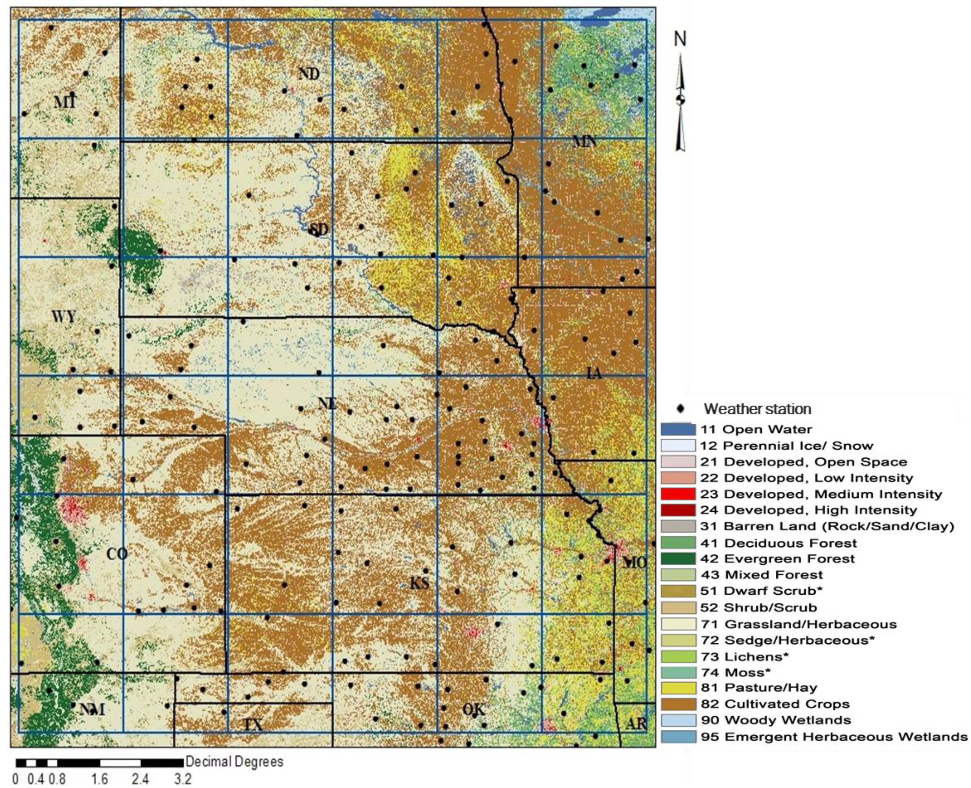
2.1. Study Area and Input Data

The study area is the High Plains region located in the central United States and extending over thirteen states: Nebraska, Kansas, South Dakota, North Dakota, Minnesota, Wyoming, Montana, Colorado, Iowa, Missouri, Oklahoma, New Mexico, and Texas (Figure 1). The region is geographically located between dense eastern forests and the western mountains and deserts [23]. The area is a vast, flat-to-rolling plain that is predominately agricultural. A landcover map of the region showing the spatial patterns of agricultural areas, natural vegetation, and urban development from the year 2006 is shown in Figure 1.
Figure 1. Map showing the study region, High Plains, the landcover during the year 2006 (Source: National Land Cover Database, and the weather stations (black dots) used in the analysis.
Climate 02 00153 g001
The study developed 2 × 2 degree grids of summer surface temperature anomalies, CO2 measurements from Mauna Loa observatory, and Advanced Very High Resolution Radiometer (AVHRR)-based NDVI. The United States Historical Climatology Network (USHCN) was the source of the monthly mean, minimum, and maximum temperature datasets for the 204 weather stations across the High Plains. The USHCN data are quality assessed by the National Climatic and Data Center (NCDC) [24]. We used the climate anomaly method (CAM) [25] to compute the monthly anomalies of the mean, minimum, and maximum temperatures for all stations. The based period used to compute the anomalies was the 30 year period of 1936 to 1965. The summer anomalies were then derived from averaging the anomalies of June, July, and August for each year. The 2 × 2 degree grid sized spatial map of anomalies over the High Plains was created by averaging the anomalies for all stations in each grid.
The atmospheric CO2 concentration data were measured at Mauna Loa, Hawaii (19.5°N; 155.6°W), and acquired from the National Oceanic and Atmospheric Administration (NOAA) Earth System Research Laboratory (ESRL). The data contain monthly mean CO2 mole fractions, expressed as parts per million (ppm). Because the measurements are made in the middle of the Pacific Ocean and at high elevations, the data are assumed to represent the mean atmospheric CO2 concentrations of a well-mixed atmosphere. The data were used to estimate the average summer CO2 atmospheric concentrations over the High Plains by averaging the concentrations of June, July, and August for every year of the study period. Prior to averaging, the CO2 concentrations for each month were standardized.
We obtained the NDVI data from Global Inventory Modeling and Mapping Studies (GIMMS). The data is originally acquired from the AVHRR sensor onboard the NOAA polar-orbiting satellites that have a biweekly temporal resolution and 4-km onboard resampled spatial grid-size. GIMMS data are resampled to 8-km pixel size products. The special features of the data include reduced NDVI variation arising from calibration, view geometry, volcanic aerosols, and other effects not related to actual vegetation change. The details on radiometric calibration, atmospheric correction and cloud screening, satellite drift correction, inter-calibration of NDVI, and quality assessment of the data are described by [26,27,28]. For this study, the data were resampled from 8-Km pixel size to 2° grids. The summer NDVI mean values were estimated from the biweekly values of June, July, and August for every year of the study period.

2.2. Spatial Gridding

The study region was gridded into 36 grids of 2° size. The grids are referenced in the figures and tables as column by row (C-R). The columns are numbered as one to six from west to east and the rows are numbered as one to six from north to south. Authors in [29] highlight that at small spatial scales, natural climatic variability is high and, thus, it is harder to detect significant anthropogenic effects on climate. Therefore, the 2° grid size was used in this study as a rational grid size that spatially does not smooth the climatological variation over the High Plains and has adaptable natural climatic variability for the optimal fingerprinting analysis.

3. ARMA Pre-Filters

The concept of maximizing the signal-to-noise ratio in the observed climate requires the assumption that the background natural climate noise is a near-stationary Gaussian process. The observed climate (such as temperature anomalies), external forcings, and natural climate noise are inherently time-dependent, which violates the stationarity assumption. The ARMA pre-filters are, therefore, designed to take into account the temporal cycles and correlation in climate data ensuring that the noise generated by projecting the observed climate into the forcing signals’ dimensional space is a near-stationary process.
Considering the observed climate (X) to be a linear combination of external forcings (Z) and natural climate noise vector (u):
X = Z β + u
where, Z = (z1|...|zt) is the matrix of external forcings (design matrix), and β = ( β1,…, βt) is vector of signal amplitudes. In this study t = 2, representing the two external forcings of CO2 concentration and LULC change (denote by NDVI). Let C be the covariance matrix of natural climate noise (u). If vector u is known, and thus C is known, by using spectral decomposition, it is possible to find a transformation pre-filter vector (A) such that: ACA' = σ2I.
Therefore C 1 = σ 2 A ' A , where I denotes the n x n identity matrix (n: being number of years of the study period), A ' is the transpose of A and σ2 is the variance of the noise vector. With the pre-filter A, Equation (1) can be transformed into:
A X = A Z β + A u
and re-parameterized as:
Y = G β + ω
where, G = AZ, Y = AX, and ω = Au is the white noise vector with covariance matrix σ2I and mean zero.
However, in this study u is unknown, therefore the first step of the procedure was to model the transformation pre-filter A such that ω is a near stationary process. To reach this assumption, first, ordinary least squares was applied on Equation (1) to generate residuals (u) as shown:
u = X   X ̂ ,   where  X ̂ = Z β ̂
Then, an ARMA model was fit on u such that the outcome was a near stationary natural climate noise ( w ) :
̂ ( B ) θ ̂ ( B ) u = w
where, ̂ ( B ) θ ̂ ( B ) is the transforming ARMA pre-filter (A). The ARMA pre-filter was fit by determining the nominator as an autoregressive model of order [p], and the denominator as a moving average model of order [q]. The orders [p]; and [q]; were determined by constructing the partial autocorrelation function (PACF) and autocorrelation function (ACF), respectively, of the estimated residuals ( u ). Further details on ARMA models and determination the orders are in [30].
The fitted ARMA pre-filter was then used to transform Equation (1) as shown below:
̂ ( B ) θ ̂ ( B ) x = β ' ̂ ( B ) θ ̂ ( B ) z + w
Letting
Y = ̂ ( B ) θ ̂ ( B ) x and G = ̂ ( B ) θ ̂ ( B ) z
the ARMA pre-filtered Equation (1) was re-parameterized as: Y = G β + ω : which is Equation (3).
Thus, Equation (3) is the model representation of the linear combination of observed climate response (Y) to external forcings (G) and natural climate noise ( ω ), onto which the optimal fingerprint technique was applied to detect the signals of external forcings, where the elements of vector (β) are the amplitudes of the external forcings.

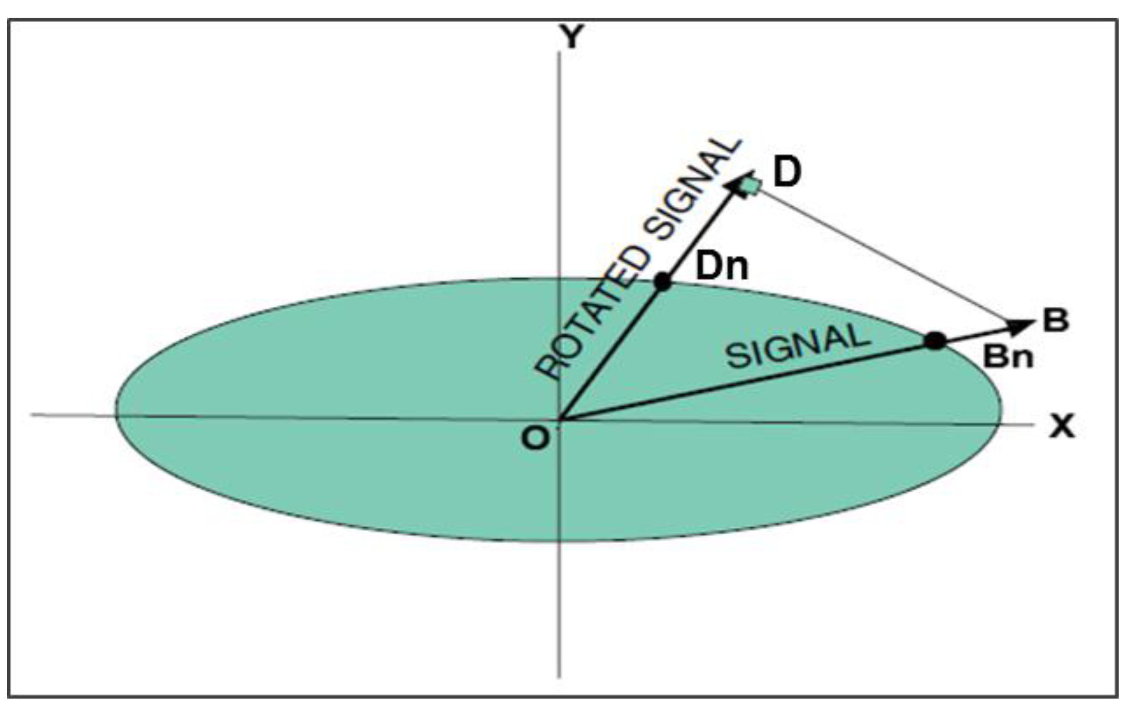
3.1. Optimal Fingerprinting Technique and Hypothesis Testing

Optimal fingerprinting is a technique that estimates the amplitude of an external forcing signal in an observed climate, [31]. Natural climate noise overwhelms the external forcing signals in observed climate data. The technique is developed to overcome this inherent problem by maximizing the distance between the signal and natural climate noise or signal-to-noise ratio [32]. We use Figure 2 to describe the concept of optimal fingerprinting: The external forcing signal (OB) in the in-situ state is usually projected in a direction space where the natural climate noise (OBn) overwhelms the statistical test of significance of the signal. Therefore, optimal fingerprinting technique re-projects the signal into a new direction space (OD) that minimizes natural climate noise (ODn), thus increasing the statistical power to detect the external forcing signal.
Figure 2. An illustration of the technique of optimal fingerprinting. The green horizontal plane represents the natural climate noise. The in-situ signal to noise ratio given by external forcing signal/ natural climate noise (OB/OBn) laying in the direction of the overwhelming natural climate noise. And the rotated signal to noise ratio new direction space/natural climate noise (OD/ODn) laying in the direction of minimized natural climate noise. The technique of optimal fingerprinting merely identifies the direction OD. Source: IPCC (2001).
Climate 02 00153 g002
The next steps of optimal fingerprinting were applied on ARMA pre-filtered and re-parameterized Equation (3) above. The determination of signal amplitudes (β) of the external forcings is the objective of the optimal fingerprinting technique. These amplitudes represent the magnitude and direction of the climate response to the external forcings. Based on the Gauss-Markov theorem, the optimal estimates of the amplitudes ( β ̂ ) , also referred to as the Best Linear Unbiased Estimators (BLUE), were estimated as.
β ̂ = ( G ' C 1   G ) 1 G ' C 1   Y
Authors in [33] referred to the ( G ' C 1  G ) 1 G ' C 1 as the operator which extracts β ̂ from Y. The intent of optimal fingerprinting is not to maximize the explained variance in observed climate response due to the external signals, but to maximize the signal to noise ratio. Therefore, authors in [34] derived a statistic equivalent to the maximized-squared-signal-to-noise-ratio (R2), which was used to test the null hypothesis of a multivariate statistical significance of an external forcing signal.
R 2 = Y ' C 1 G ( G ' C 1 G ) 1 G ' C 1 Y
where R 2 is a chi-square (χ2) variable with p degrees of freedom. The null hypothesis is that:
Ho = 0 vs. Ha : β 0, in other words, the observed climate change originates only from natural climate noise. The null hypothesis test was rejected when:
R 2 > χ t ,   1 α 2
where, χ t ,   1 α 2   is the critical value and α (0.05) is the set level of significance for the test. If one or both of the signals were not significant, then each external forcing signal was tested individually by reducing the G matrix to one dimension. Since C was estimated, the test is only reasonable if the number years is large enough. In this analysis, the study period was 26 years (1981–2006).

4. Results and Discussion

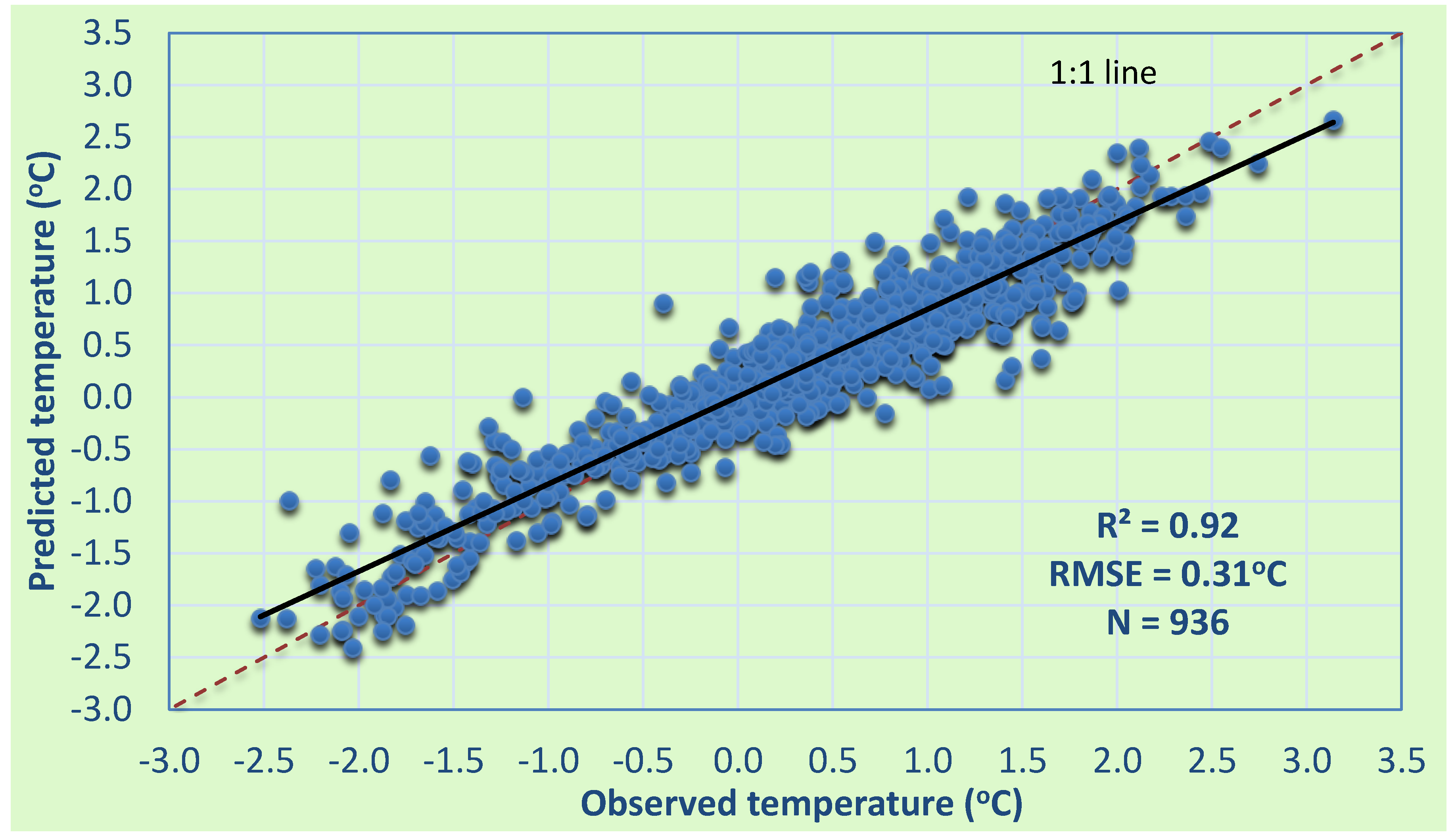
4.1. Model Fitting on Observed Summer Temperature Data

This section discusses the performance of fitted models in predicting the observed temperature anomalies during the study period. It is observed in Figure 3 that the model predicted anomalies practically agreed with observed temperature anomalies, with a coefficient of determination (r2) of 0.92 and Root Mean Square Error (RMSE) of 0.31. The year 1992 had the lowest anomalies (<−1.5). The cooling of summer 1992 has been associated with volcanic aerosol-induced cooling of the global mean temperature due to the June 1991 Pinatubo eruption in the Philippines [35]. The warmest anomalies (>2.0) were from the year 1988 due to the extreme dry and hot drought that lasted from 1987 to 1989. According to [36] the drought of 1988 covered 36% of USA at its peak. The cooling and warming of temperatures during the summers of 1992 and 1988, respectively, demonstrate the impact of the natural forcings in masking out external forcing signals and trends on climate. Such large events in natural climate variability make statistical detection of external forcing signals practically impossible. The suppression of these events by subtracting or modeling them out of natural climate variability could simplify the estimation of the undisturbed or “normal” natural climate variability, thus enhancing the detection of external forcing signals. Indeed, authors in [33] minimized the impact of volcanic activities of Mt. Agung and Mt. Pinatubo in detection analysis by omitting the data over the period effected by the events.

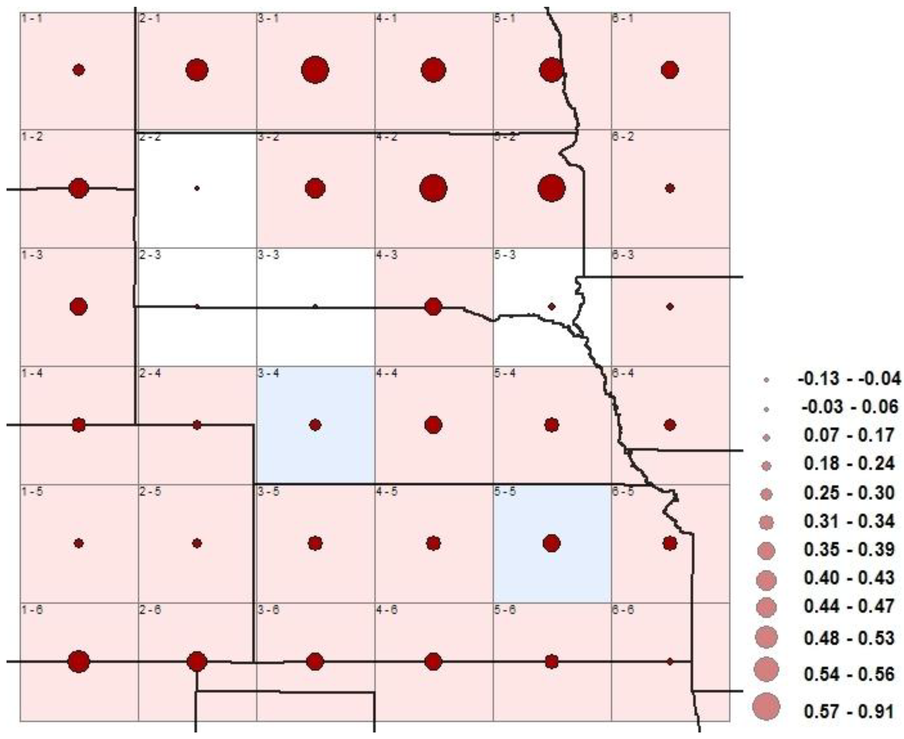
4.2. Spatial Signatures of Climate Response to LULC Changes Using NDVI Proxy

The spatial signatures of optimally estimated signal amplitudes of LULC changes are presented in Figure 4. The relative magnitude of the amplitude in each grid is represented by the solid cycle that is referenced the legend of the figure. Statistically, the amplitudes are estimates of the main effect of the LULC changes forcing on the observed temperature anomalies. The positive or negative sign of the amplitude indicates whether the external forcing on temperature was a warming or cooling effect, respectively. Since the amplitudes appear mostly negative in Figure 4, the effect of LULC changes on the regional temperature is mostly a cooling effect. The blue grids in Figure 4 show areas with significant a LULC change cooling effect on the regional temperatures, with both NDVI and CO2 forcings in the model. The light blue grids show areas with significant cooling effect, but with only NDVI forcing in the model. That is, when both NDVI and CO2 forcings were in the model, the NDVI signal was insignificant, however when CO2 was dropped from the model, the signal of NDVI became significant. The change in significance or even direction of a signal when another signal is added to or dropped from the model is referred to as multicollinearity [37]. Multicollinearity is caused by probable presence of correlation between forcing signals, making it difficult to identify and interpret the signals that have the most effect.
Figure 3. Model-predicted temperature anomalies vs. observed temperature anomalies. “N” is the number of points. RMSE: root mean square difference.
Climate 02 00153 g003
In Figure 4, the red colored grids are areas where the LULC change forcings yielded a significant positive or warming effect. These grids are mostly covered with natural vegetation and grassland for cattle ranching. The white grids represent areas where LULC change forcing had an insignificant effect. Probably due to the natural climate variability completely overwhelming the LULC change signal or due to inadequate evidence to detect the LULC change signal on observed temperature in those grids. For instance, in Grid 1–5, which covers most of the areas on the eastern slopes of the Rocky Mountains, the elevation of the weather stations ranged between 1600 and 2800 m above mean sea level. The temperature measurements of these stations are most likely to be mainly influenced by topographic and high elevation effect. Additionally, the area is subjected to periodic, severe turbulent conditions from the effects of high westerly Chinook winds over the mountain barrier. The winds are highly episodic, thus tremendously noisy, which makes the extraction of external forcing signals on measured temperatures practically difficult to detect statistically. Importantly, due to the grid size used in this study, the exact spatial extent of the significant or insignificant signatures of the forcings in the region is coarsened. These results are only representative of the average spatial patterns of climate response to LULC change forcing over the High Plains during the 26 years of this study. The signatures of climate response to LULC changes and CO2 forcings are not temporally and spatially stationary over the years, but rather physically dynamic, evolving spatially and in significance as seasons, natural forcings (such as solar and volcanic activities, ENSO, droughts, etc.), and other external forcings influence the climate in the region.
Figure 4. Spatial signatures of climate response to NDVI effect on the High Plains’ regional climate. Blue grids indicate areas with significant cooling signal, white grids indicate areas with insignificant NDVI signal, and light blue grids indicate areas with significant cooling signal from one-signal pattern model. Red grids indicate areas with significant warming signal. The solid green and red circles represent the magnitude of the amplitudes of NDVI signal in each grid.
Climate 02 00153 g004
The widespread cooling effect in Figure 4 is probably due to the evaporative cooling originating from the extensive irrigation in the region. A study by [38] using RegCM2 revealed a warming hole (minimum warming) in the High Plains that was attributed to evaporative cooling suppressing daytime maximum temperatures of the region during the summer months of June, July, and August. In fact the warming hole was observed to start developing in June, reaching its maximum value in September and gradually diminishing through October and November. The months of June, July, August, and September are characterized by extensive irrigation in the High Plains. A similar climate change study by [39] using the global Community Climate System Model Version 3 (CCSM3) earth systems model also shows the projected July temperatures between 2000 and 2050 to be increasing at a slower rate in the High Plains relative to surrounding regions, especially the western Region.
The irrigated area in the High Plains has steadily increased from about 8 million ha in 1980 to more than 13.4 million ha by 2000. This trend has continued into the 21st century as economical profitability and other incentives of maize, soybean, wheat, and other crops have led farmers to convert natural grasslands of the High plains into irrigated croplands. Studies [10,40,41,42,43,44] have shown that irrigation and vegetation coverage have a direct influence on regional surface temperatures. These studies show that irrigation can consistently reduce maximum daily temperatures by as much as 7.5 °C. In a simulation study by [45] more evidence was provided on the impact of agricultural-related land use change on the surface climate of the High plains. In some regions (Nebraska) they observed a significant irrigation-induced surface cooling effect of 1.2 °C.

4.3. Spatial Signatures of Climate Response to Greenhouse Gases Using CO2 as Proxy

The main purpose of including atmospheric CO2 forcing in the model was to suppress the radiative effect of greenhouse gases from the observed climate, thus enhancing the LULC change signal to noise ratio. Atmospheric CO2 concentration has often been used to express the net radiative forcing contribution of anthropogenic greenhouse gases on the climate [46]. The spatial signatures of optimally estimated amplitudes of CO2 are presented in Figure 5. The solid circles in the grids also represent the relative magnitude of the estimated amplitudes of the atmospheric CO2 signal. Compared with the LULC change amplitudes, the CO2 amplitudes were mainly positive, indicating a radiative warming effect on regional climate of the High Plains. The red colored grids show areas with a significant radiative warming effect. The two blue colored grids (3–4 and 5–5) indicate areas with a significant cooling effect. Four white grids (2–2, 2–3, 3–3, and 5–3) had an insignificant CO2 radiative effect on the regional climate. The magnitudes of the amplitudes of these grids were indeed the smallest, an indication that the atmospheric CO2 signal in these areas was weak. Grids 2–2 and 3–3 also had insignificant LULC change signals which raised the possibility that the natural climate variability in the observed temperature of these areas completely overwhelmed both signals of LULC changes and atmospheric CO2 concentrations or the observed temperature in the two grids had insufficient footprints of the two external forcings.
Since we used global atmospheric CO2 concentrations from Mauna Loa, Hawaii, the variation in the spatial signatures of climate response to atmospheric CO2 forcing was not expected to fluctuate much over the region. However, in Figure 5, the amplitudes of atmospheric CO2 signals were observed to be strongest in the northern part relative to the rest of the region. In a recent study by [47], the trends in average annual temperatures over the region also show the strongest amount of warming to be in North Dakota and the least in Colorado. The warming signal of atmospheric CO2 forcing was observed to be weakest in the central part of the High Plains and appears to increase again from the central part towards the south. In Figure 5, the amplitudes of atmospheric CO2 forcing are smaller in magnitude compared to LULC changes amplitudes. The optimal fingerprinting technique automatically assigns higher weights to variables with high signal-to-noise ratio [48]. These results, therefore, indicate that the atmospheric CO2 signal in the region was weak compared to the LULC changes signal. Authors in [42] observed that the expanding evaporative cooling from irrigation over the past years might have introduced a countervailing temperature effect, limiting the detection of global greenhouse warming signal in observational records of temperature. Our results and recent studies, such as [38,42,49], demonstrate that the regional climatic effect originating from anthropogenic induces an atmospheric-biosphere interaction attributed to LULC change, which is probably masking the global greenhouse gas radiative warming in the High Plains region.
Figure 5. Spatial signatures of climate response to CO2 radiative effect on the High Plains’ regional climate. Red grids indicate areas with significant warming signal, white grids indicate areas with insignificant CO2 signal, and blue grids indicate areas with significant cooling signal. The solid red circles represent the magnitude of the amplitudes of CO2 signal in each grid.
Climate 02 00153 g005

5. Conclusions

By integrating ARMA modeling and the optimal fingerprinting technique, an enhanced signal processing procedure was developed to detect the signals of LULC changes on the regional climate of the US High Plains. The ARMA pre-filters were used as linear transformation models that ensured the output residuals were near-stationary processes, thus enforcing the assumption of stationarity of natural climate variability. The study used NDVI as a proxy of LULC changes and atmospheric CO2 concentrations as a proxy of greenhouse gases. The results, which are representatives of the average spatial signatures of climate response to LULC change forcing on the regional climate of the High Plains during the 26 years of the study period, show a significant cooling effect on the regional climate during the summer season. The cooling effect is probably due to the evaporative cooling originating from the increasing extensive irrigation in the region. Atmospheric CO2 forcing was added into the model to suppress the radiative effect of greenhouse gases, thus enhancing the LULC change signal to noise ratio. The results show that the greenhouse gas warming effect was mostly significant in the region, but weak compared to LULC change signal. This study demonstrates the regional climatic impact of anthropogenic induced atmospheric-biosphere interaction attributed to LULC change, which is an additional important climate forcing besides greenhouse gas radiative forcing in the High Plains region.

Author Contributions

All authors have contributed to the idea and hypothesis development, method development, analyses, interpretation of the results and writing the manuscript.

Conflicts of Interest

The authors declare no conflict of interest.

References

  1. Mahmood, R.; Pielke, R.A.; Hubbard, G.K.; Niyogi, D.; Bonan, G.; Lawrence, P.; Mcnider, R.; Mcalpine, C.; Etter, A; Gameda, S. Impacts of land use/land cover change on climate and future research priorities. Bull. Amer. Meteorol. Soc. 2010, 91, 37–46. [Google Scholar]
  2. Chase, T.N.; Pielke, R.A., Sr.; Kittel, T.G.F.; Nemani, R.R.; Running, W.S. Simulated impacts of historical land cover changes on global climate in northern winter. Clim. Dyn. 2000, 16, 93–105. [Google Scholar] [CrossRef]
  3. Kalnay, E.; Cai, M. Impact of urbanization and land use on climate change. Nature 2003, 423, 528–531. [Google Scholar] [CrossRef] [PubMed]
  4. Cai, M.; Kalnay, E. Response to the comments by Vose et al. and Trenberth. Nature 2004. [Google Scholar] [CrossRef]
  5. Trenberth, K.E. Rural land-use change and climate. Nature 2005. [Google Scholar] [CrossRef]
  6. Vose, R.S.; Karl, T.R.; Easterling, D.R.; Williams, C.N.; Menne, M.J. Impact of land-use change on climate. Nature 2004, 427, 213–214. [Google Scholar] [CrossRef] [PubMed]
  7. Feddema, J.J.; Oleson, K.W.; Bonan, G.B.; Mearns, L.O.; Buja, L.E.; Meehl, G.A.; Washington, W.M. The importance of land-cover change in simulating future climates. Science 2005, 310, 1674–1678. [Google Scholar] [CrossRef] [PubMed]
  8. Christy, J.R.; Norris, W.B.; Redmond, K.; Gallo, K.P. Methodology and results of calculating central California surface temperature trends: Evidence of human-induced climate change? J. Clim. 2006, 19, 548–563. [Google Scholar]
  9. Mahmood, R.; Keeling, T.; Hubbard, K.G.; Carlson, C.; Leeper, R. Impacts of irrigation on 20th century temperatures in the Northern Great Plains. Global Planet. Change 2006, 54, 1–18. [Google Scholar] [CrossRef]
  10. Mahmood, R.; Pielke, R.A., Sr.; Hubbard, K.; Niyogi, D.; Dirmeyer, P.; McAlpine, C.; Carleton, A.; Hale, R.; Gameda, S.; Beltrán-Przekurat, A.; et al. Land cover changes and their biogeophysical effects on climate. Int. J. Climatol. 2014, 34, 929–953. [Google Scholar] [CrossRef]
  11. Ezber, Y.; Sen, O.L.; Kindap, T.M.; Karaca, M. Climatic effects of urbanization in Istanbul: A statistical and modeling analysis. Int. J. Climatol. 2007, 27, 667–679. [Google Scholar] [CrossRef]
  12. De Noblet-Ducoudré, N.; Boisier, J.P.; Pitman, A.J.; Bonan, G.B.; Brovkin, V.; Cruz, F.; Delire, C.; Gayler, V.; van den Hurk, B.J.J.M.; Lawrence, P.J.; et al. Determining robust impacts of land-use induced land-cover changes on surface climate over North America and Eurasia: Results from the first of LUCID experiments. J. Clim. 2011, 25, 3261–3281. [Google Scholar] [CrossRef]
  13. Cotton, W.R.; Pielke, R.A., Sr. Human Impacts on Weather and Climate; Cambridge University Press: New York, NY, USA, 1995. [Google Scholar]
  14. Guillevic, P.C.; Privette, J.L.; Coudert, B.; Palecki, M.A.; Demarty, J.; Ottle, C.; Augustine, J.A. Land Surface Temperature product validation using NOAA’s surface climate observation networks—Scaling methodology for the Visible Infrared Imager Radiometer Suite (VIIRS). Remote Sens. Environ. 2012, 124, 282–298. [Google Scholar] [CrossRef]
  15. Houghton, J.T.; Ephraums, J.J. Climate Change: The IPCC Scientific Assessment; Cambridge University Press: New York, NY, USA, 1990. [Google Scholar]
  16. Hasselmann, K. On the signal-to-noise problem in atmospheric response studies. In Meteorology of Tropical Oceans; Shawn, D.B., Ed.; Royal Meteorological Society: London, UK, 1979; pp. 251–259. [Google Scholar]
  17. Barnett, T.P.; Schlesinger, M.E. Detecting changes in global climate induced by greenhouse gases. J. Geophys. Res. 1997, 92, 14772–14780. [Google Scholar] [CrossRef]
  18. Santer, B.D.; Wigley, T.M.L.; Schlesinger, M.E.; Jones, P.D. Greenhouse-Gas-Induced Climatic Change. In Multi-Variate Methods for a Detection of Greenhouse-Gas-Induced Change: A Critical Appraisal of Simulations and Observations; Elsevier: Amsterdam, The Netherland, 1991; pp. 511–536. [Google Scholar]
  19. Santer, B.D.; Bruggermann, W.; Cubasch, U.; Hasselmann, K.; Hock, H.; Maier-Reimer, E.; Mikolajewicz, U. Signal-to-noise analysis of time-dependent greenhouse warming experiments. Part 1: Pattern analysis. In Max-Planck-Institut Fur Meteorogie Report 98; Max-Planck Institut for Meteorologie Bundesstrasse: Hamburg, Germany, 1993; pp. 46–62. [Google Scholar]
  20. Cubasch, U.; Santer, B.D.; Hellach, A.; Hegerl, G.; Hӧck, H.; Maier-Reimer, E.; Mikolajewicz, U.; Stassl, A. Monte Carlo climate change forecasts with a global coupled ocean-atmosphere model. Clim. Dyn. 1994, 10, 1–19. [Google Scholar]
  21. Hasselmann, K. PIPs and POPs: The reduction of complex dynamical systems using principal interaction and oscillation patterns. J. Geophys. Res. 1988, 93, 11015–11021. [Google Scholar] [CrossRef]
  22. Von Storch, H.; Bruns, T.; Fischer-Bruns, I.; Hasselmann, K. Principal oscillation pattern analysis of the 30- to 60-day oscillation in a general circulation model equatorial troposphere. J. Geophys. Res. 1988, 93, 11022–11036. [Google Scholar] [CrossRef]
  23. Rossum, S.; Lavin, S. Where are the Great Plains? A cartographic analysis. Prof. Geogr. 2000, 52, 543–552. [Google Scholar] [CrossRef]
  24. Smith, T.M.; Reynolds, R.W.; Peterson, T.C.; Lawrimore, J. Improvements to NOAA’s historical merged land-ocean surface temperature analysis (1880–2006). J. Clim. 2008, 21, 2283–2293. [Google Scholar] [CrossRef]
  25. Jones, P.D. Hemispheric surface air temperature variations: A reanalysis and an update to 1993. J. Clim. 1994, 7, 1794–1802. [Google Scholar] [CrossRef]
  26. Pinzon, J. Using HHT to successfully uncouple seasonal and interannual components in remotely sensed data. In Proceedings of the SCI 2002 Conference, Orlando, FL, USA, 14–18 July 2002.
  27. Pinzon, J.; Brown, M.E.; Tucker, C.J. Satellite time series correction of orbital drift artifacts using empirical mode decomposition. In Hilbert-Huang Transform: Introduction and Applications; Huang, N.E., Shen, S.S., Eds.; World Scientific: Hackensack, NJ, USA, 2004; pp. 17–29. [Google Scholar]
  28. Tucker, C.J.; Pinzon, J.E.; Brown, M.E.; Slayback, D.; Pak, E.W.; Mahoney, R.; Vermote, E.; Nazmi, E.S. An extended AVHRR 8-km NDVI dataset compatible with MODIS and SPOT vegetation NDVI data. Int. J. Remote Sens. 2005, 26, 4485–4498. [Google Scholar] [CrossRef]
  29. Sexton, M.H.D.; Grubb, H.; Shine, P.K.; Folland, K.C. Design and analysis of climate model experiments for the efficient estimation of anthropogenic signals. J. Clim. 2003, 16, 1320–1336. [Google Scholar] [CrossRef]
  30. Shumway, R.H.; Stoffer, D.S. Time Series Analysis and Its Applications: With R Examples, 2nd ed.; Springer: New York, NY, USA, 2006. [Google Scholar]
  31. Allen, M.R.; Stott, P.A. Estimating signal amplitudes in optimal fingerprinting (I), Theory. Clim. Dyn. 2003, 21, 477–491. [Google Scholar] [CrossRef]
  32. Levine, A.R.; Berliner, M.L. Statistical principles for climate change studies. J. Clim. 1999, 12, 564–574. [Google Scholar] [CrossRef]
  33. Allen, M.R.; Tett, S.F.B. Checking for model consistency in optimal fingerprinting. Clim. Dyn. 1999, 15, 419–434. [Google Scholar] [CrossRef]
  34. Hasselmann, K. Optimal fingerprints for the detection of time dependent climate change. J. Clim. 1993, 6, 1957–1971. [Google Scholar] [CrossRef]
  35. Hansen, J.; Lacis, A.; Ruedy, R.; Sato, M. Potential climate impact of Mountain Pinatubo eruption. Geophys. Res. Lett. 1992, 19, 215–218. [Google Scholar] [CrossRef]
  36. Riebsame, W.E.; Changnon, S.A.; Karl, T.R. Drought and Natural Resources Management in the United States: Impacts and Implications of the 1987–1989 Drought; Westview Press: Boulder, CO, USA, 1991. [Google Scholar]
  37. Judge, G.G.; Griffiths, W.E.; Hill, R.C.; Lutkepohl, H.; Lee, T.C. The Theory and Practice of Econometrics, Second Edition; John Wiley & Sons: New York, NY, USA, 1985. [Google Scholar]
  38. Pan, Z.; Arritt, R.W.; Takle, E.S.; Gutowski, W.J., Jr.; Anderson, C.J.; Segal, M.M. Altered hydrologic feedback in a warming climate introduces a “warming hole”. Geophys. Res. Lett. 2004. [Google Scholar] [CrossRef]
  39. Ganguly, A.R.; Parish, E.S.; Singh, N.; Steinhaeuser, K.; Erickson, D.J.; Branstetter, M.L.; King, A.W.; Middleton, E.J. Regional and decadal analysis of climate change induced extreme hydro-meteorological stresses informs adaptation and mitigation policies. In Proceedings of the 21st Conference on Climate Variability and Change, Phoenix, AZ, USA, 13 January 2009.
  40. Pielke, R.A., Sr.; Pitman, A.; Niyogi, D.; Mahmood, R.; McAlpine, C.; Hossain, F.; Goldewijk, K.; Nair, U.; Betts, R.; Fall, S.; et al. Land use/land cover changes and climate: Modeling analysis and observational evidence. WIREs Clim. Change 2011. [Google Scholar] [CrossRef]
  41. Lobell, D.; Bala, G.; Mirin, A.; Phillips, T.; Maxwell, R. Regional differences in the influence of irrigation on climate. J. Clim. 2009, 22, 2248–2255. [Google Scholar] [CrossRef]
  42. Kueppers, L.M.; Snyder, M.A.; Sloan, L.C. Irrigation cooling effect: Regional climate forcing by land-use change. Geophys. Res. Lett. 2007. [Google Scholar] [CrossRef]
  43. Bonfils, C.; Lobell, D. Empirical evidence for a recent slowdown in irrigation-induced cooling. Proc. Natl. Acad. Sci. USA 2007, 104, 13582–13587. [Google Scholar] [CrossRef] [PubMed]
  44. Boucher, O.; Myhre, G.; Myhre, A. Direct human influence of irrigation on atmospheric water vapor and climate. Clim. Dyn. 2004, 22, 597–603. [Google Scholar] [CrossRef]
  45. Adegoke, J.O.; Pielke, R.A., Sr.; Carleton, A.M. Observational and modeling studies of the impacts of agriculture-related land use change on climate in the central U.S. Agric. For. Meteorol. 2007. [Google Scholar] [CrossRef]
  46. Houghton, J.T.; Meira Filho, L.G.; Callander, B.A.; Harris, N.; Kattenberg, A.; Maskell, K. Climate Change 1995: The IPCC Second Scientific Assessment; Cambridge University Press: Cambridge, UK, 1996. [Google Scholar]
  47. High Plains Regional Climate Center (HPRCC). Climate Change on the Prairie: A Basic Guide to Climate Change in the High Plains Region. Available online: http://www.hprcc.unl.edu/publications/files/HighPlainsClimateChangeGuide.pdf (accessed on 7 January 2012).
  48. Hegerl, G.C.; von Storch, H.; Hasselmann, K.; Santer, B.D.; Cubasch, U.; Jones, P.D. Detecting greenhouse gas-induced climate change with an optimal fingerprint method. J. Clim. 1996, 9, 2281–2306. [Google Scholar] [CrossRef]
  49. Pitman, A.J.; de Noblet-Ducoudre, N.; Cruz, F.T.; Davin, E.L.; Bonan, G.B.; Brovkin, V.; Claussen, M.; Delire, C.; Ganzeveld, L.; Gayler, V.; et al. Uncertainties in climate responses to past land cover change: First results from the LUCID intercomparison study. Geophys. Res. Lett. 2009. [Google Scholar] [CrossRef]

