
Assessing Property Exposure to Cyclonic Winds under Climate Change
by
 ,
,
Evelyn G. Shu
1,* ,
,
Mariah Pope
1,
Bradley Wilson
1,
Mark Bauer
1,
Mike Amodeo
1,
Neil Freeman
1 and
Jeremy R. Porter
1,2 1
First Street Foundation, Brooklyn, NY 11201, USA
2
Department of Sociology and Demography, City University of New York, New York, NY 10017, USA
*
Author to whom correspondence should be addressed.
Climate 2023, 11(11), 217; https://doi.org/10.3390/cli11110217
Submission received: 14 August 2023
/
Revised: 25 October 2023
/
Accepted: 29 October 2023
/
Published: 1 November 2023
Abstract
:Properties in the United States face increasing exposure to tropical storm-level winds due to climate change. Driving this increasing risk are severe hurricanes that are more likely to occur when hurricanes form in the future and the northward shift of Atlantic-formed hurricanes, increasing the estimated exposure of buildings and infrastructure to damaging winds. The wind model presented here combines open data and science by utilizing high-resolution topography, computer-modeled hurricane tracks, and property data to create hyper-local tropical cyclone wind exposure information for the Contiguous United States (CONUS) from current time to 2053 under RCP 4.5. This allows for a detailed evaluation of probable wind speeds by several return periods, probabilities of cyclonic thresholds being reached or surpassed, and a comparison of this cyclone-level wind exposure between the current year and 30 years into the future under climatic changes. The results of this research reveal extensive exposure along the Gulf and Southeastern Atlantic Coasts, with significant growing exposure in the Mid-Atlantic and Northeastern regions of the country.
1. Introduction
Tropical storms and hurricanes are types of severe weather systems (tropical cyclones) that form over and gain their energy from warm ocean waters. By definition, tropical storms have sustained wind speeds of 39–73 mph, while hurricanes have wind speeds of 74 mph or higher [1]. The wind speed of tropical cyclones is used to classify these storms on the Saffir–Simpson scale, ranging from tropical storms to hurricanes, with Category 1 hurricanes being the weakest and Category 5 storms being the strongest. Tropical storms and hurricanes are both dangerous and destructive, and people in at-risk areas should prepare for potential impacts. In the contiguous United States (CONUS), the Gulf and East Coasts face the highest probabilities of tropical cyclone winds that can cause significant damage to properties and infrastructure.
Physical property damage from tropical cyclones has been rising in the United States and is expected to continue rising in the future [2]. Winds from tropical cyclones (hurricanes and tropical storms) can cause significant damage to property and infrastructure, disrupt essential services, and pose a serious threat to human life. Tropical cyclone winds span large areas, reach high speeds, and are accompanied by heavy rainfall, which can cause destructive flooding. Notably, hurricanes affect communities within the United States more frequently and severely than other natural disasters [3]. As a result, tropical cyclones have caused a total of USD 1.194 trillion (CPI adjusted) in losses in the United States between 1980 and 2022 (see Figure 1), with an average cost of approximately USD 21 billion per event. Of the approximately USD 41–70 billion in losses due to Hurricane Ian in 2022, it is estimated that half of those damages (USD 23–35 billion) were due to wind damage [4]. Additionally, the annual economic costs have increased during each of the last four decades [2]. Given the increasing damage estimates from tropical cyclones, there is a need to evaluate the probable changes in wind exposure in the future in order to provide US residents with an informed understanding of their risk.
Over the next 30 years, tropical cyclones are more likely to become major hurricanes, with greater intensities, and therefore, their effects will reach further inland. While the total number of such storms is not expected to increase in the future due to a changing climate, the frequency of major hurricanes (Category 3–5) relative to the total number of hurricanes that form is expected to increase over time [5]. In other words, the intensity of the hurricanes that develop in the future is expected to increase (see Figure 2). Wang and Toumi [6] report that the number of tropical cyclones with landfall intensity of more than 50 m s−1 has doubled since the 1980s. In the North Atlantic, the proportion of major hurricanes has increased by four times since the 1980s, from about 10% of all tropical cyclone events to over 40% of all events today [7]. Driving this increase in intensity are rising air temperatures that increase the temperatures and heat the upper layers of the ocean waters, which provide the energy that fuels these storms. Li and Chakraborty [8] presented that in recent years, tropical cyclones tend to decay more slowly after landfall.
Other environmental changes, including increases in the amounts of moisture in the atmosphere and alterations to large-scale wind patterns, also influence the intensity of hurricanes and where they are likely to move. Over the next 30 years, tropical cyclones will push further northward before making landfall. A shift of storms poleward has already been observed in the global historical data and has been confirmed by modeling studies, which means that the probability of storms making landfall further north along the East Coast of the US is expected to increase (see Figure 3) [9]. While wind exposure is most significant along the coast, it is likely to increase inland drastically in many places that have never before been exposed.
While tropical cyclone wind events are most common and severe along the Gulf Coast, they pose significant risk to many parts of the United States, particularly along the East Coast. Communities with greater awareness of their risk may take precautions, such as imposing more stringent building codes, which result in structures that better withstand high wind velocities. However, areas unaccustomed to these risks or unaware of future increases in exposure may be unprepared for wind impacts. As the probability and severity of tropical cyclone activities increase in these areas, more people, property, infrastructure, and economic resources are exposed. Furthermore, since hurricanes that will form in the future are more likely to be severe storms, the cyclone-level winds resulting from a landfalling hurricane will also extend further into the interior of the US (see Figure 4), as it will take longer for storms’ wind speeds to decrease after the source of their energy—warm ocean waters—has been cut off at landfall.
In order to assess this increasing exposure, this research develops a national wind exposure model using open data, open science, and engineering expertise to create a tropical cyclone wind model that assesses hyper-local climate tropical cyclone wind speed exposure across the CONUS due to the Atlantic-formed cyclones. This research focuses on the Atlantic-formed tropical cyclones, as Pacific cyclones tend not to make landfall on the West Coast of the United States due to cooler water temperatures. The wind model uses high-resolution topography, computer-modeled hurricane tracks, and property data to allow for a detailed evaluation of probable wind speeds by return period and a comparison of this wind exposure between the current year and 30 years in the future under RCP 4.5.
The Intergovernmental Panel on Climate Change (IPCC) presents a framework for understanding risk through the necessary components of hazard, exposure, and vulnerability [10]. Hazard refers to the probability and severity of physical environmental events, while exposure refers to the assets, people, and systems that are located within those hazard fields. The final component necessary to constitute risk is vulnerability, which encompasses the factors (for example, social, economic, and political factors) that influence the susceptibility of an exposed system to impacts and the ability to cope with or recover from events [10].
Current and future exposure to wind from hurricanes and tropical storms is calculated in this manuscript by using the modeled tropical cyclone tracks to estimate wind speeds at a 10 km horizontal resolution for the CONUS. The hazard information provided by the wind model relies on information from approximately 50,000 synthetic hurricane tracks created by computer models and based on historical storms to enable robust statistical sampling of hurricanes’ characteristics [11]. These synthetic tracks and their concomitant wind fields are downscaled using surface roughness corrections at the 30 m resolution for multiple return periods and are projected 30 years into the future using the World Climate Research Programme (WCRP) Climate Model Intercomparison Project 6 (CMIP6) climate models (WCRP) [12]. These are then combined with property data across the CONUS to better understand the property-level impacts and exposure due to cyclonic winds. Taken together, this research contributes to our understanding of cyclonic wind exposure implications by building on existing research through the development of high-resolution exposure estimates (30 m), standardizing hazard information across multiple return periods, and adjusting this exposure into the future using existing global climate models. Additionally, this manuscript complements the existing literature [13] that considers the same source of modeled synthetic tracks to evaluate the associated flood risk.
The wind exposure model indicates that extensive exposure to high winds is expected along the Gulf and Southeastern Atlantic Coasts. While these regions have historically been prone to tropical cyclones, hurricanes, and other severe weather events, the model also reveals growing exposure in the Mid-Atlantic and Northeastern regions of the country, especially along the inland stretch, which has mild exposure in the current climate. Overall, in the next 30 years, 13.4 million properties are likely to face tropical cyclone-level winds that do not currently face such exposure.
2. Methodology
2.1. Hurricane Tracks
The wind model uses large numbers (~104) of synthetic hurricane tracks derived under current (2015–2030) and future (2079–2099) CMIP6-defined climatic conditions. Hurricane tracks for the wind model were provided by Rhodium Group and WindRiskTech LLC and generated using methods that have been described in detail in previous peer-reviewed publications and validated well against historical observations [11,14,15,16,17]. We describe the methodology in brief below but refer readers to the original publications for a more detailed description of the tropical cyclone downscaling model used for the track generation.
The track generation process starts with a monthly representation of the mean thermodynamic conditions for a given climate state, defined with sea surface temperature and air temperature and humidity at all model levels up through the lower stratosphere from a GCM or reanalysis. Daily winds at the 250-hPA and 850-hPA levels are used to create a synthetic time series of winds at both levels that are constrained to have the same monthly means, variances, and covariances as the global model, and a power spectrum that falls off with the cube of the frequency. Weak protocyclonic disturbances are then introduced randomly in space and time and allowed to move according to the weighted mean of the 250- and 850-hPa flow and a correction for beta drift [18]. The hurricane intensity is integrated along each track via the Coupled Hurricane Intensity Prediction System (CHIPS), a highly resolved coupled ocean–atmosphere model solved in angular momentum coordinates [14]. During this process, most of the protocyclonic disturbances die off and are discarded; the remaining disturbances that amplify to at least tropical storm intensity then define the tropical cyclone climatology of the given model.
Tracks from seven CMIP6 GCMs under scenario SSP245 were used in the wind model (Table A1). The models selected include the GCMs that WindRiskTech has deemed adequate representations of the climate conditions necessary for studying tropical cyclone hazards. SSP245 is used as a middle-of-the-road climate scenario. For each GCM, 50 tracks per year that made landfall in the CONUS with the least tropical storm intensity were generated for both the current (2015–2030) and end-of-century (2079–2099) scenarios. To more accurately characterize the tails of the hurricane intensity distribution, an additional 25 tracks per GCM/year were generated using a higher intensity threshold. As a final layer of variance, every track was replicated into two additional ensemble members with slightly different storm characteristics. These included track paths that were jittered based on a statistically informed random walk of the original path and pressure and radii values that were randomly sampled from a lognormal distribution [19]. Combining all ensemble members resulted in 3600 and 4735 unique storms per GCM in the current/future periods for a total universe of 58,345 unique hurricane tracks. An example subsample of a track set is shown in Figure 4.
2.2. Wind Field Modeling
In order to capture spatially heterogeneous wind velocities at specific locations, we used a combination of an axisymmetric gradient wind field model [20] and a boundary layer model [21] to produce spatially continuous estimates of 10 m sustained 1 min wind fields for each synthetic hurricane track on a fixed grid with 0.1-degree cell resolution. Sustained winds refer to the wind speeds sustained for a minimum of 1 min, resulting from the circulation within a tropical cyclone, which are used to classify hurricane categories by intensity. This process builds upon the pre-processed synthetic hurricane tracks described in Section 2.1. All wind field modeling and calculations were performed using a set of MATLAB scripts originally provided by WindRiskTech and modified for application to the wind model.
The wind field modeling workflow requires the specification of one or more points of interest (POI) and a pre-processed synthetic track set. For the wind model, fourteen unique GCM-timeframe combinations (7 GCMs under current and future conditions) were used. To define the area of influence for the hurricane component of the wind model, we ran the wind field modeling procedure for an initial set of POIs located at the centroids of 1.0 × 1.0-degree tiles across CONUS. Any tile that received tropical storm wind speeds or above in at least one hurricane track was subsequently split into 0.1-degree grid cells and included in the production POI list.
Given a POI and track set, surface wind speeds were derived in the following steps. First, a radial profile of gradient wind from Emanuel and Rotuno [20] was fitted to the model-predicted peak gradient wind speed and radius of maximum winds, including the effects of secondary eyewalls. This profile was then modified to account for storm translation and the effects of environmental wind shear. The track set was then filtered to events that passed within 750 km of the point of interest at any point along their paths. This reduced the computational time needed for a given simulation by excluding tracks that did not produce winds at the POI. The wind speed and direction at the POI location were calculated at thirty-minute time steps for each track, using the wind field described above and the distance between the track and the POI. The wind speeds were converted into 1 min sustained surface wind speeds at 10 m height for each time step using surface drag coefficients. The surface drag coefficient data are natively stored at 25 km horizontal resolution and interpolated to the point of interest. This step accounts for the spindown of the hurricane vortices over cold land and the decay of surface winds over rough terrain.
The wind field workflow returns matrices of wind speed and direction for every storm in the event set. We generated 1 min sustained wind estimates for all POIs across all fourteen hurricane track sets. For each scenario, the wind speed matrices were filtered to return the maximum surface wind speed for each track. The wind direction matrices were converted into frequency distribution tables showing the percentage of storms at the POI across eight cardinal directions in 45-degree bands. We restricted the direction calculations to only include storms reaching hurricane intensity (>74 mph).
2.3. Wind Hazard Statistics
To generate return period and frequency statistics for each POI, we started with Track IDs from sampling tables that contained 1000 simulated time series of tropical cyclones in a given year (2015–2099) for each GCM and scenario. The sampling tables were constructed by randomly selecting Track IDs into a given yearly time series using the baseline hazard information associated with each track, then allowing for each track to have an equal probability chance to randomly swap to either one of its ensemble members. For years between the 2015–2030 and 2079–2099 track sets, the sampling tables pull a linear combination of track IDs from both current and future track sets, with increasing contributions from the end-of-century storms as the years increase. This process mixes the temporal pattern seen in sea level rise with the stable signals in GCM changes over the century. We focused on the 2015–2030 and 2045–2060 time periods for the wind model.
For each grid cell, we drew the maximum surface wind speed corresponding to the Track IDs across all 1000 simulations in the sampling table and generated frequency counts in 10 mph bins from 0 mph to 220 mph. These are converted annual exceedance probabilities under a Poisson distribution:
where μ is the counting rate, and t is the time period of interest. These 10 mph binned values are interpolated with cubic splines to return the wind speeds corresponding to specific 2-, 5-, 20-, 100-, 300-, 500-, 700-, 1700-, and 3000-year return periods (see Figure 5 for the 3000-year return period outputs). To account for year-to-year variability across the current and future scenarios, the statistics for each year within a given time window were weighted using the average number of landfalling storms across the synthetic time series relative to the entire population of storms. This process was repeated for the track sets from each GCM.
Due to variability in the climate conditions within the GCMs, the simulated hurricane tracks and resulting windfields showed significant variation in location and magnitude across climate models, even after thousands of simulations (Table 1). As a general rule, for statistics in the wind risk model, we used an ensemble mean with equal weights on all seven GCMs. For instances in lower return periods (2-year and 5-year) where less than seven models contained wind speed information at every POI, we ensembled the average of all available GCMs, provided at least two were available.
2.4. Surface Roughness
The hurricane wind field model does not account for the hyper-local effects of surface roughness on wind speeds. Very rough areas, such as suburban or heavily forested areas, can decrease wind speeds, while open terrain can increase wind speeds. At the hyper-local scale, we implemented a surface roughness correction to the hurricane wind field model output (1 min sustained wind speeds and direction) with local terrain data.
We started with surface roughness length information (z0) at a 30 m resolution derived from the FEMA Hazus Hurricane Model [22]. A z0 value ranges from 0.003 m (open water) to 1.5 m (center of a tall city) and represents the effect of obstructions and vegetation on the shape of the boundary layer wind velocity profile. The z0 values from HAZUS [22] are segmented by land cover classifications within the U.S. Geological Survey National Land Cover Database (NLCD) [23] and state or regional classifications. In states without z0 coefficients, we used the mean values per land cover class. To account for the separate regions in Florida and New York, we used the county boundaries that most closely matched each region.
To model the potential effects of surrounding terrain on wind speeds, we calculated a moving average to represent the ground surface roughness around any given structure. We used exposure categories from the American Society for Civil Engineers (ASCE) [24] guidelines for wind loads on building exposures to determine the averaging radius. We used the “Exposure B” calculations to determine the radii at which to take the moving averages, as Exposure B is defined as urban and suburban areas, wooded areas, or other terrain with numerous closely spaced obstructions having the size of single-family dwellings or larger. Additionally, it is estimated that the majority of buildings have an exposure category that is considered Exposure B [25].
For Exposure B, the ground surface roughness values prevail for the following distances:
- Buildings with a mean roof height of less than or equal to 30 ft = 1500 feet radius;
- Buildings with a mean roof height of greater than 30 ft = 2600 feet radius.
Based on this guidance, we created circular moving average raster layers from the 30 m z0 values at both a 1500 ft and 2600 ft radius. We also created eight moving average rasters for both radii in 45-degree directional windows to account for how wind speeds might vary depending on the direction of approach (see Figure 6 for surface roughness examples for Miami-Dade County, FL).
The final z0 values were then used to adjust the modeled wind speeds for local roughness effects. Wind speeds at different heights in the vertical wind profile were extracted using the power law, which can be defined as follows:
where v_z represents the wind speed at height z; v_g represents the wind speed at height z_g, and n is the power law exponent related to the wind speeds at heights z and z_g that will incorporate surface roughness. The power law is then applied to the exposure coefficient (k_z) in ASCE7 as a factor that allows for the type and height of exposure to be applied to gust loads. The equation for the exposure coefficient for any structure above 15 feet is defined as
where z is the height of interest (10 m); is the wind shear exponent that depends on z0, and z_g is the gradient layer height. It can then be assumed that this equation implies that the wind velocity profiles can take the form of
where z_g and are defined as
where
where
2.5. Calculating Property Exposure
Property boundaries (obtained from Lightbox) [26] are spatially joined with the surface roughness data and resulting wind information. Each property is assigned a wind speed based on applying surface roughness coefficients for each direction to the speed produced by the model, then weighting based on the percentage of hurricane-force winds from each direction. If a property has more than 75% of winds coming from a single direction, we instead use the circular average surface roughness to avoid the edge cases where only a few hurricane tracks contribute to the direction information.
The maximum speed information is calculated by considering the maximum speeds expected for all of the return periods considered by the wind model. Return periods reflect the probabilities associated with possible wind events, where an event that has a 5% probability of occurring in a given year is referred to as having a 20-year return period; an event that has a 1% probability of occurring in a given year is referred to as a 100 years return period event, and so on. The wind model estimates what these events will look like for this year and in 30 years for the 2-, 5-, 20-, 100-, 300-, 500-, 700-, 1700-, and 3000-return periods. Low likelihood return periods, such as the 1700- and 3000-year return periods, are important to characterize as these are the most severe events and are considered for engineering design standards. For example, the ASCE considers the 300-, 700-, 1700-, and 3000-year return periods in their standards [27]. The probabilities of reaching or exceeding specific speeds may also be calculated as the probability of experiencing different cyclonic storm category-level winds each year. For example, this allows for the calculation of the probability of experiencing Category 1 hurricane-level winds or higher in a given year.
The adjusted wind speeds are then converted from 1 min sustained winds into a 3 s gust by averaging across the four gust-factor curves presented in Vickery and Skerlj [28]. The 3 s wind gusts result from small-scale variations within a storm and are typically the cause of maximum wind damage to properties. The gust factor for converting winds from 60 s to 3 s comes out to 1.28.
3. Results
3.1. Overview of National Patterns
In the Northeast, there is a concentration of properties that will be newly exposed to some probability of tropical storm-level winds or higher in 30 years. The Mid-Atlantic will see the largest increase in maximum wind speeds in CONUS over the next 30 years, with some areas increasing in maximum speeds by 37 mph. Some areas within this region can anticipate relatively large increases in the probability of experiencing a hurricane over the next 30 years when compared to today, with many areas expected to see an additional 1% annual probability. See Figure 7 for a map of the states impacted by these regional differences.
To identify the areas with the most severe exposure to cyclonic-level winds, the maximum wind speed that each area is likely to experience in the current year is displayed in Figure 8a. While these wind speeds will not necessarily occur in any given year, this probabilistic approach allows for a calculation of what maximum speeds are expected in the worst-case scenario, up to the ASCE guidance for building code thresholds at the extreme 3000-year return period (equivalent to a 0.03% of annual chance of occurring, or 1% over a 30-year mortgage).
Figure 8c illustrates how wind exposure will be changing over the next 30 years under the modeled outputs for the current year and 30 years into the future. Although Louisiana has a concentration of the highest maximum gust speeds (approximately 248 mph), South Carolina is expected to face the largest increase in maximum wind speeds over the next 30 years (+37 mph; see Figure 8c). Additionally, much of the Mid-Atlantic sees relatively large increases in the probability of exposure to hurricane wind speeds, increasing by an additional 1% annual likelihood. Interestingly, inland states like Illinois, Kentucky, and Tennessee will also experience significant increases relative to their current levels, with gust speeds in Tennessee increasing from 87 mph to 97 mph.
While the number of exposed properties stays relatively constant below the 300-return period, the impact of climate change is evident in the higher return periods. For instance, in the 3000-return period, there are 13.4 million additional properties exposed in 30 years that are not today, which represents a 15.6% percent increase. Figure 9 shows a breakdown of how many properties in the CONUS may be exposed to tropical cyclone winds in each of these return periods for the current year and for 30 years. The overall number of properties exposed in the lower return periods (the 2- and 5-year return periods) is expected to decrease somewhat as storms shift northward and exposure decreases in some areas around the Gulf.
The number of properties exposed to different hurricane categories will also change over the next 30 years. In the current year, there are about 3.5 million properties within the CONUS with any chance of experiencing Category 5 hurricane winds, but in 30 years, this number will increase to over 5.6 million properties (Figure 10). Additionally, there are about 10.3 million properties with any chance of experiencing Category 4 hurricane wind conditions this year, increasing to approximately 14.9 million properties that could be exposed to those wind conditions in 30 years. This illustrates the impact of the previously mentioned results that hurricanes that form in the future in a changing climate are expected to increase proportionally in severity.
3.2. Exposure to Tropical Cyclone Wind Speeds
The counties exposed to the highest maximum wind speeds in the 500-year return period for the current year are listed in descending order in Table 2. The list is topped by counties in Louisiana, Texas, and Florida. The highest maximum speeds are expected in St. Bernard, LA (wind gusts up to 218 mph); Plaquemines, LA (wind gusts up to 215 mph); Monroe, FL (wind gusts up to 212 mph); Galveston, TX (wind gusts up to 211 mph); and Terrebonne, LA (wind gusts up to 209 mph). The top ten county list is rounded out by Iberia, LA; Lafourche, LA; Chambers, TX; Vermilion, LA; and Miami-Dade, FL, respectively.
The counties expected to see the largest increase in maximum wind gust speeds in the 500-year return period (Table 3) are primarily in Virginia, with some counties in South Carolina, Georgia, and North Carolina making the top 20 county list. Jasper, SC, will see the largest increase in wind gust speeds in the 500-year return period, increasing by approximately 15 mph. Rounding out the top five include Amelia, VA; Goochland, VA; Chesterfield, VA; and Culpeper, GA, respectively.
The breakdown of properties exposed to different tropical cyclone categories within each return period is shown in Figure 11 for this year and in 30 years.
Under current environmental conditions, about 11.6 million properties are exposed to the chance of a Category 1 hurricane or higher in the 20-year return period. That means that, for approximately 11.6 million properties in the CONUS, there is a cumulative probability of about 79% of being exposed to at least one Category 1 hurricane over the span of a 30-year mortgage. All probabilities of various tropical cyclone winds (for example, “the probability of exposure to Category 1 winds”) refer to the likelihood of reaching at least that speed. An area beginning in the Gulf Coast and stretching northward along the East Coast toward the Northeast has a significant chance of a Category 1 storm or higher reaching it. The highest probabilities of exposure to a Category 1 storm this year are focused along the Gulf Coast, with some areas exceeding a 27% likelihood this year (Figure 12a). In 30 years, while the spatial patterns remain fairly similar, some areas around the Gulf may see a slight decrease in their annual probabilities of experiencing a hurricane (Figure 12b), which illustrates the northward shift of hurricanes over the next 30 years due to a changing climate.
Understanding how the probabilities of exposure to hurricane winds change between this year and 30 years in the future allows for adequate planning for resilient communities. A holistic understanding of wind exposure over the next 30 years allows the communities to plan investment opportunities, risk mitigation, and building-hardening strategies. In 30 years, the counties with the highest probabilities of experiencing hurricane winds are again topped by Monroe, FL; Miami-Dade, FL; Collier, FL; Broward, FL; and Palm Beach, FL. The rest of the top 20 list for county probabilities of hurricane winds are similar to those of the current year and are made up primarily of counties in Florida and Louisiana.
The counties that will likely face the greatest absolute increase in their annual likelihood of experiencing Category 1 hurricane wind conditions (Table 4) include Gloucester, VA; Isle of Wight, VA; York, VA; Mathews, VA; and Poquoson, VA, respectively.
4. Discussion
The wind model presented in this research represents multiple advances in our understanding of wind exposure by introducing a climate-adjusted tropical cyclone wind model at the property level. This model gives property owners an objective view of their personal exposure to tropical cyclone-level wind now and in the future and can be used to make personal decisions about where to live, adaptation solutions, and property-hardening against that exposure. This model incorporates changing climate conditions as a way to predict changes in hurricane exposure over the next 30 years. Understanding how wind exposure changes over time with future environmental conditions at a high spatial resolution is important to know how financial, human, and community resources should be allocated in order to mitigate the risks associated with hurricane winds.
Areas that may be newly exposed to severe tropical cyclone winds or those that have an increased likelihood of experiencing severe wind events may be at particular risk if building standards are reliant on past or current day exposure levels. Important implications associated with these results center around a community’s ability to assess current levels of resilience, plan for future resource allocation around infrastructure and development, and inform individuals of their personal risks. For example, even though inland areas will likely experience lower wind speeds than coastal regions, this exposure is significant given that these inland states may not be fully aware of future expected wind speed increases, which could ultimately result in increased damage during hurricane wind condition events.
Areas that face the largest increases in maximum wind speeds over the next 30 years may not be prepared for damaging wind events, as building codes are typically defined by historical events and not future predicted probabilities of maximum wind speeds. This is especially true for areas that may face relatively low maximum wind speeds in the current year, as they will cross over damaging wind speed thresholds sometime over the next 30 years. The impact of such changes in wind gust speeds on properties could be drastic as the expected damage increases.
More specifically, this research works to quantify and understand the changes that are occurring in the environment and then translates and communicates those changes at the property level. The use of these research results to identify relative exposure between areas and under different probabilistic scenarios helps inform decisions around community resilience and future development. Additionally, identifying areas with high relative exposure may allow for the appropriate allocation of resources so that capital is used efficiently and development decisions do not necessarily lead to the unintentional location of vulnerable populations and properties in highly exposed areas.
Author Contributions
Conceptualization, M.P., B.W., M.A. and E.G.S.; methodology, M.P., B.W., M.A. and E.G.S.; software, N.F.; validation, M.P. and B.W.; formal analysis, M.P., B.W. and M.B.; investigation, M.P.; data curation, M.P., B.W., N.F. and M.B.; writing—original draft preparation, E.G.S., M.P., B.W. and J.R.P.; writing—review and editing, E.G.S., M.P., B.W., M.A. and J.R.P.; visualization, M.B.; supervision, M.A. and B.W. All authors have read and agreed to the published version of the manuscript.
Funding
This research received no external funding.
Data Availability Statement
The input datasets used for this analysis are either already publicly available or cannot be made available due to restrictive data sharing agreements.
Conflicts of Interest
The authors declare no conflict of interest.
Appendix A

Table A1.
Global Climate Models used in the wind model.
| Model Name: | Model Origin: | Model Agency: |
|---|---|---|
| MPI6 | Germany | Max Planck Institute |
| MRI6 | Japan | Meteorological Research Institute, Japan |
| MIROC6 | Japan | Atmosphere and Ocean Research Institute (The University of Tokyo), National Institute for Environmental Studies, and Japan Agency for Marine-Earth Science and Technology |
| ECEARTH | Europe | EC-Earth Consortium |
| UKMO6 | United Kingdom | Hadley Centre for Climate Prediction and Research |
| NORESM6 | Norway | NorESM Climate modeling Consortium (NCC) |
| CESM2 | USA | National Center for Atmospheric Research (NCAR) |
References
- NOAA. Hurricanes. 2020. Available online: https://www.noaa.gov/education/resource-collections/weather-atmosphere/hurricanes (accessed on 12 January 2023).
- NOAA. National Centers for Environmental Information (NCEI) U.S. Billion-Dollar Weather and Climate Disasters (2023). Available online: https://www.ncei.noaa.gov/access/billions/ (accessed on 12 January 2023).
- Cutter, S.L.; Emrich, C. Are natural hazards and disaster losses in the US increasing? EOS Trans. Am. Geophys. Union 2005, 86, 381–389. [Google Scholar] [CrossRef]
- CoreLogic. Estimated Losses from Hurricane Ian Wind, Storm Surge are Between $28 Billion and $47 Billion in Costliest Florida Storm Since Hurricane Andrew. CoreLogic. 2022. Available online: https://www.corelogic.com/press-releases/corelogic-estimated-losses-from-hurricane-ian-wind-storm-surge-are-between-28-billion-and-47-billion-in-costliest-florida-storm-since-hurricane-andrew/ (accessed on 12 January 2023).
- Knutson, T.R.; Sirutis, J.J.; Garner, S.T.; Vecchi, G.A.; Held, I.M. Simulated reduction in Atlantic hurricane frequency under twenty-first-century warming conditions. Nat. Geosci. 2008, 1, 359–364. [Google Scholar] [CrossRef]
- Wang, S.; Toumi, R. More tropical cyclones are striking coasts with major intensities at landfall. Sci. Rep. 2022, 12, 5236. [Google Scholar] [CrossRef] [PubMed]
- Kossin, J.P.; Knapp, K.R.; Olander, T.L.; Velden, C.S. Global increase in major tropical cyclone exceedance probability over the past four decades. Proc. Natl. Acad. Sci. USA 2020, 117, 11975–11980. [Google Scholar] [CrossRef] [PubMed]
- Li, L.; Chakraborty, P. Slower decay of landfalling hurricanes in a warming world. Nature 2020, 587, 230–234. [Google Scholar] [CrossRef] [PubMed]
- Kossin, J.P.; Emanuel, K.A.; Vecchi, G.A. The poleward migration of the location of tropical cyclone maximum intensity. Nature 2014, 509, 349–352. [Google Scholar] [CrossRef] [PubMed]
- Reisinger, A.; Howden, M.; Vera, C.; Garschagen, M.; Hurlbert, M.; Kreibiehl, S.; Mach, K.J.; Mintenbeck, K.; O’Neill, B.; Pathak, M.; et al. The Concept of Risk in the IPCC Sixth Assessment Report: A Summary of Cross-Working Group Discussions; Intergovernmental Panel on Climate Change: Geneva, Switzerland, 2020.
- Emanuel, K.; Ravela, S.A.; Vivant, E.A.; Risi, C.A. A Statistical-Deterministic Approach to Hurricane Risk Assessment. Bull. Amer. Meteor. Soc. 2006, 87, 299–314. [Google Scholar] [CrossRef]
- Eyring, V.; Bony, S.; Meehl, G.A.; Senior, C.A.; Stevens, B.; Stouffer, R.J.; Taylor, K.E. Overview of the Coupled Model Intercomparison Project Phase 6 (CMIP6) experimental design and organization. Geosci. Model Dev. 2016, 9, 1937–1958. [Google Scholar] [CrossRef]
- Bates, P.D.; Quinn, N.; Sampson, C.; Smith, A.; Wing, O.; Sosa, J.; Savage, J.; Olcese, G.; Neal, J.; Schumann, G.; et al. Combined modeling of US fluvial, pluvial, and coastal flood hazard under current and future climates. Water Resour. Res. 2021, 57, e2020WR028673. [Google Scholar] [CrossRef]
- Emanuel, K.; DesAutels, C.; Holloway, C.; Korty, R. Environmental control of tropical cyclone intensity. J. Atmos. Sci. 2004, 61, 843–858. [Google Scholar] [CrossRef]
- Emanuel, K.A. Downscaling CMIP5 climate models shows increased tropical cyclone activity over the 21st century. Proc. Natl. Acad. Sci. USA 2013, 110, 12219–12224. [Google Scholar] [CrossRef] [PubMed]
- Emanuel, K. Effect of upper-ocean evolution on projected trends in tropical cyclone activity. J. Clim. 2015, 28, 8165–8170. [Google Scholar] [CrossRef]
- Emanuel, K. Climate and tropical cyclone activity: A new model downscaling approach. J. Clim. 2006, 19, 4797–4802. [Google Scholar] [CrossRef]
- Marks, D.G. The beta and advection model for hurricane track forecasting; NOAA Technical Memorandum NWS NMC 70. Release: Washington, DC, USA, 1992.
- Chavas, D.R.; Emanuel, K.A. A QuikSCAT climatology of tropical cyclone size. Geophys. Res. Lett. 2010, 37, L18816. [Google Scholar] [CrossRef]
- Emanuel, K.; Rotunno, R. Self-Stratification of Tropical Cyclone Outflow. Part I: Implications for Storm Structure. J. Atmos. Sci. 2011, 68, 2236–2249. [Google Scholar] [CrossRef]
- Vickery, P.J.; Wadhera, D.; Powell, M.D.; Chen, Y. A Hurricane Boundary Layer and Wind Field Model for Use in Engineering Applications. J. Appl. Meteorol. Climatol. 2009, 48, 381–405. [Google Scholar] [CrossRef]
- Federal Emergency Management Agency (FEMA). HAZUS Hurricane Model Technical Manual, HAZUS 5.1. 2021. Available online: https://www.fema.gov/sites/default/files/documents/fema_hazus-hurricane-model-technical-manual-5-1.pdf (accessed on 12 January 2023).
- US Geological Survey (USGS). National Land Cover Database (NLCD) 2019 Products, version 2.0; US Geological Survey Data Release: Reston, VA, USA, 2021.
- ASCE Standard ASCE/SEI 7-22; Minimum Design Loads for Buildings and Other Structures. American Society of Civil Engineer: Reston, VA, USA, 2022.
- Ho, E. Variability of Low Building Wind Lands. Ph.D. Thesis, University of Western Ontario, London, ON, Canada, 1992. [Google Scholar]
- Lightbox. Lightbox Property Data. 2023. Available online: https://www.lightboxre.com/data/ (accessed on 15 February 2023).
- McAllister, T.P.; Wang, N.; Ellingwood, B.R. Risk-informed mean recurrence intervals for updated wind maps in ASCE 7-16. J. Struct. Eng. 2018, 144, 06018001. [Google Scholar] [CrossRef] [PubMed]
- Vickery, P.J.; Skerlj, P.F. Hurricane Gust Factors Revisited. J. Struct. Eng. 2005, 131, 825–832. [Google Scholar] [CrossRef]
Figure 1.
Billion-Dollar Tropical Cyclone Disasters (CPI Adjusted 2022 USD).

Figure 2.
Proportion of major hurricanes by year in the North Atlantic Ocean and Gulf of Mexico, from historical observations [7]. This is a triad time series (3 year bins) of the global fractional proportion of major hurricane intensities to all hurricane intensities.
Figure 2.
Proportion of major hurricanes by year in the North Atlantic Ocean and Gulf of Mexico, from historical observations [7]. This is a triad time series (3 year bins) of the global fractional proportion of major hurricane intensities to all hurricane intensities.

Figure 3.
Mean absolute storm latitude from global modeled storms under historical conditions (green line) and future conditions (black line) from Dr. K. Emanuel (personal communication, February 2023).
Figure 3.
Mean absolute storm latitude from global modeled storms under historical conditions (green line) and future conditions (black line) from Dr. K. Emanuel (personal communication, February 2023).
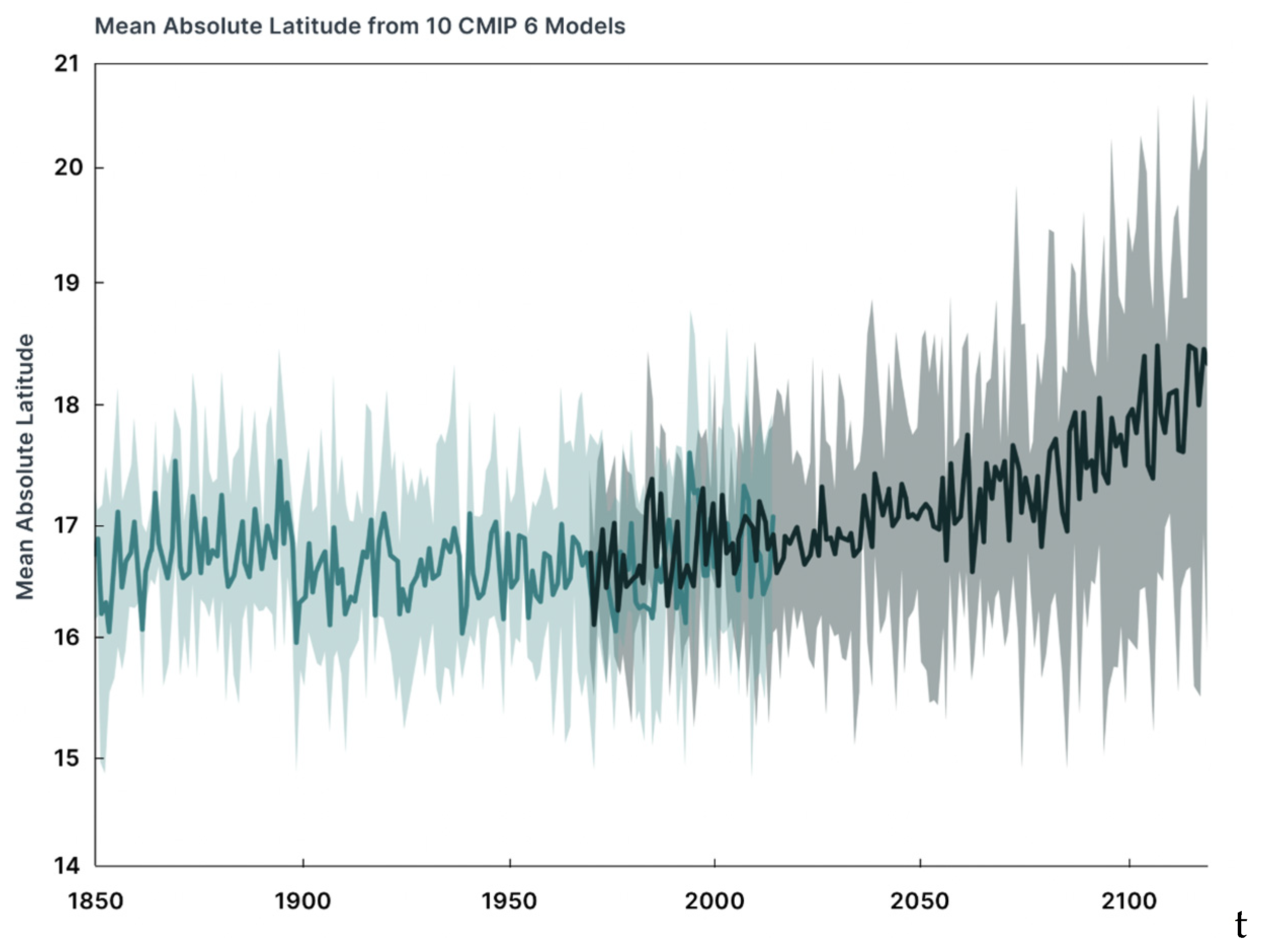
Figure 4.
Sample of 50 hurricane tracks from the CESM2 Global Climate Model for the current time period (2015–2030).
Figure 4.
Sample of 50 hurricane tracks from the CESM2 Global Climate Model for the current time period (2015–2030).
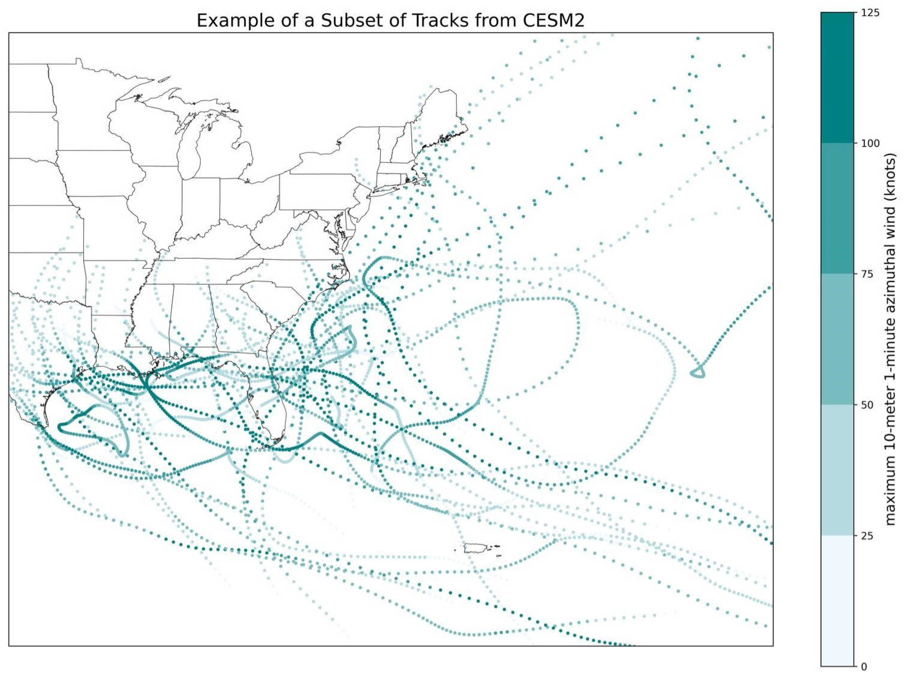
Figure 5.
Wind speed estimate at RP 3000 based on the GCM ensemble mean.

Figure 6.
Surface roughness examples for Miami-Dade County.

Figure 7.
Regional differences in tropical cyclone wind exposure from the application of the wind model.
Figure 7.
Regional differences in tropical cyclone wind exposure from the application of the wind model.

Figure 8.
Maximum, and change in maximum, wind gust speeds from the wind model. (a) Maximum wind speed in 2023. (b) Maximum wind speed in 2053. (c) Increase in maximum wind speed.
Figure 8.
Maximum, and change in maximum, wind gust speeds from the wind model. (a) Maximum wind speed in 2023. (b) Maximum wind speed in 2053. (c) Increase in maximum wind speed.


Figure 9.
Percent of properties exposed to tropical cyclones by return period.
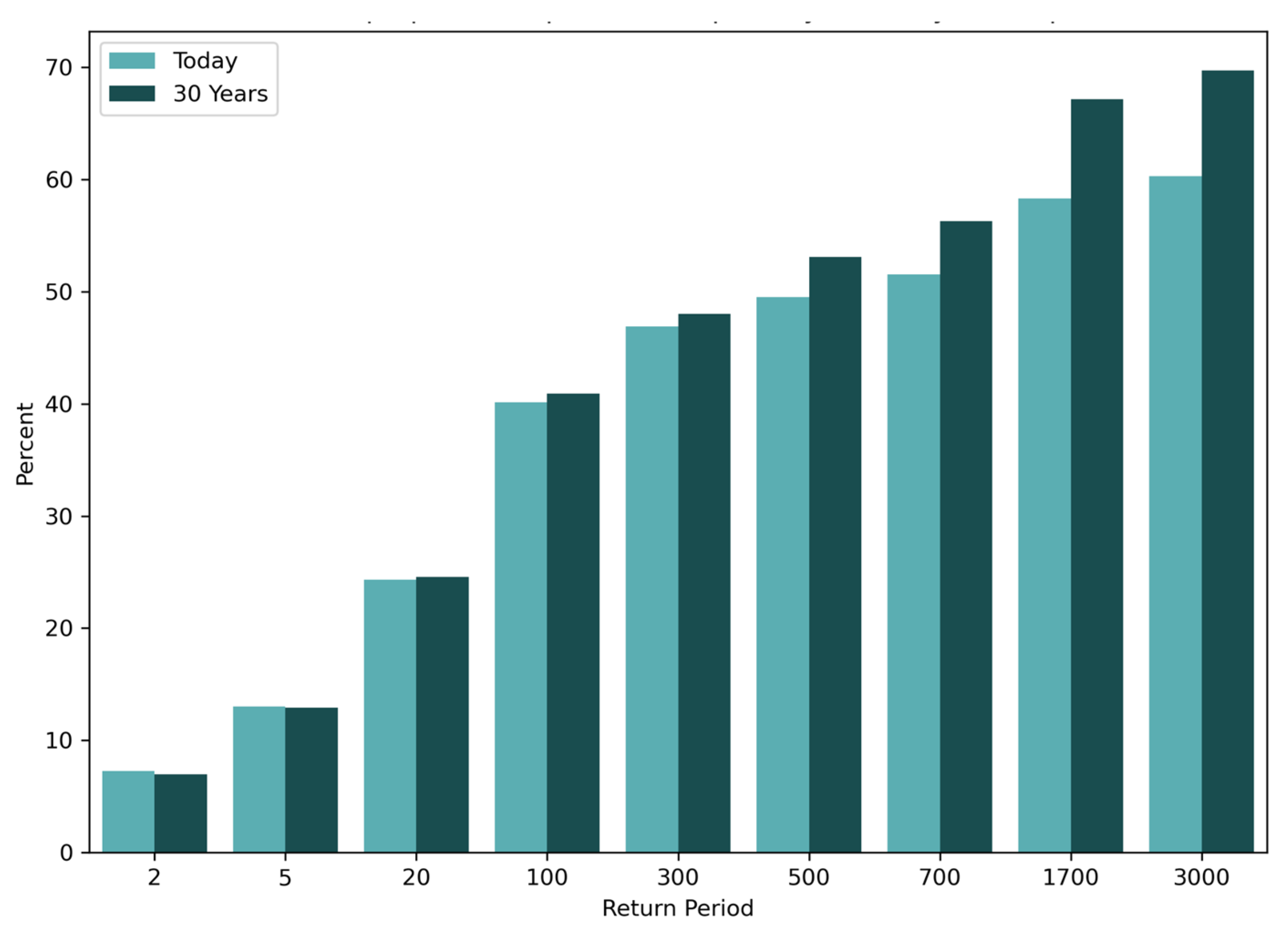
Figure 10.
Percent of properties exposed to Category 5 hurricane winds by return period today and in 30 years.
Figure 10.
Percent of properties exposed to Category 5 hurricane winds by return period today and in 30 years.

Figure 11.
Number of properties exposed to storm categories within different return periods for 2023 (a) and 2053 (b).
Figure 11.
Number of properties exposed to storm categories within different return periods for 2023 (a) and 2053 (b).

Figure 12.
Probability of exposure to Category 1 hurricane winds (a) 2023 and (b) 2053.
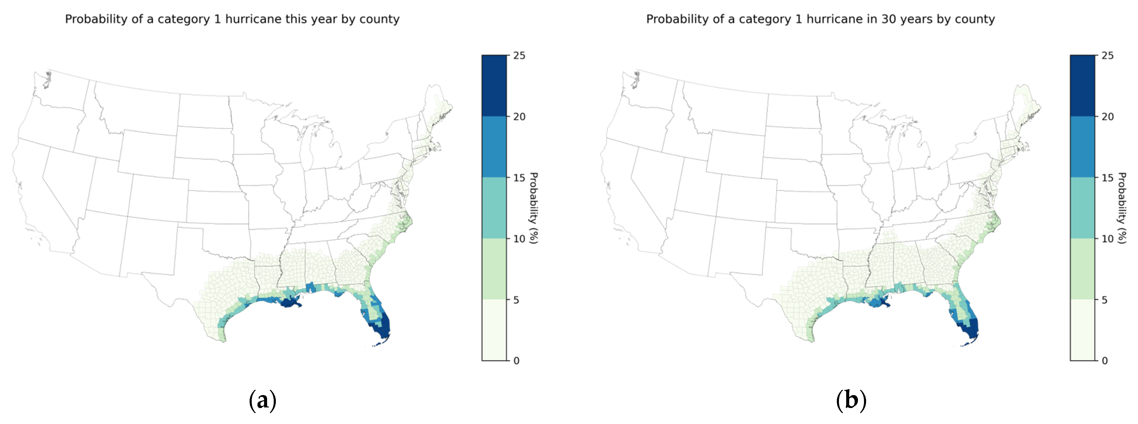
Table 1.
Global Climate Models used in the wind model.
| Model Name | Model Origin | Model Agency |
|---|---|---|
| MPI6 | Germany | Max Planck Institute |
| MRI6 | Japan | Meteorological Research Institute, Japan |
| MIROC6 | Japan | Atmosphere and Ocean Research Institute (The University of Tokyo), National Institute for Environmental Studies, and Japan Agency for Marine-Earth Science and Technology |
| ECEARTH | Europe | EC-Earth Consortium |
| UKMO6 | United Kingdom | Hadley Centre for Climate Prediction and Research |
| NORESM6 | Norway | NorESM Climate Modeling Consortium (NCC) |
| CESM2 | USA | National Center for Atmospheric Research (NCAR) |
Table 2.
Top counties by expected wind gust speeds (mph).
| Wind Gust Speeds (mph) by Return Period and Year | ||||||||||
|---|---|---|---|---|---|---|---|---|---|---|
| County | RP 5 (2023) | RP 5 (2053) | RP 20 (2023) | RP 20 (2053) | RP 100 (2023) | RP 100 (2053) | RP 500 (2023) | RP 500 (2053) | RP 3000 (2023) | RP 3000 (2053) |
| St. Bernard, LA | 92 | 90 | 133 | 131 | 182 | 179 | 218 | 218 | 230 | 242 |
| Plaquemines, LA | 99 | 95 | 141 | 138 | 183 | 182 | 215 | 218 | 232 | 244 |
| Monroe, FL | 102 | 99 | 141 | 138 | 183 | 180 | 212 | 215 | 230 | 244 |
| Galveston, TX | 90 | 87 | 131 | 128 | 175 | 174 | 211 | 214 | 232 | 244 |
| Terrebonne, LA | 96 | 93 | 137 | 136 | 179 | 180 | 209 | 215 | 228 | 244 |
| Iberia, LA | 91 | 88 | 133 | 133 | 179 | 182 | 209 | 216 | 228 | 247 |
| Lafourche, LA | 96 | 92 | 138 | 136 | 179 | 179 | 207 | 211 | 221 | 239 |
| Chambers, TX | 87 | 84 | 128 | 125 | 172 | 173 | 207 | 211 | 227 | 241 |
| Vermilion, LA | 88 | 87 | 131 | 132 | 175 | 179 | 207 | 214 | 227 | 243 |
| Miami-Dade, FL | 101 | 97 | 138 | 137 | 180 | 180 | 207 | 212 | 229 | 242 |
| Jefferson, TX | 88 | 86 | 127 | 127 | 172 | 173 | 207 | 210 | 228 | 237 |
| Orleans, LA | 87 | 84 | 127 | 124 | 173 | 170 | 207 | 210 | 225 | 239 |
| St. Mary, LA | 90 | 87 | 129 | 129 | 174 | 177 | 206 | 211 | 227 | 242 |
| Cameron, LA | 88 | 86 | 127 | 128 | 172 | 173 | 206 | 211 | 225 | 238 |
| Collier, FL | 100 | 97 | 138 | 137 | 177 | 174 | 206 | 212 | 224 | 238 |
| Jefferson, LA | 95 | 92 | 138 | 134 | 179 | 178 | 206 | 211 | 221 | 239 |
| Broward, FL | 100 | 97 | 137 | 134 | 175 | 174 | 206 | 211 | 227 | 239 |
| Palm Beach, FL | 100 | 96 | 136 | 133 | 172 | 173 | 205 | 209 | 227 | 238 |
| St. Tammany, LA | 87 | 83 | 125 | 123 | 172 | 166 | 205 | 207 | 223 | 238 |
| Harrison, MS | 87 | 83 | 127 | 124 | 173 | 169 | 204 | 205 | 219 | 230 |
Footnote: Table is sorted by the highlighted column RP 500 (2023).
Table 3.
Top counties by increase in max wind gust speeds (mph).
| County | RP 500 Wind Gust (2023) | RP 500 Wind Gust (2053) | Change in RP 500 Wind Gust | RP 3000 Wind Gust (2023) | RP 3000 Wind Gust (2053) | Change in RP 3000 Wind Gust |
|---|---|---|---|---|---|---|
| Jasper, SC | 155 | 170 | 15 | 170 | 207 | 37 |
| Amelia, VA | 73 | 87 | 14 | 84 | 108 | 23 |
| Goochland, VA | 72 | 86 | 14 | 81 | 102 | 22 |
| Chesterfield, VA | 83 | 97 | 14 | 95 | 115 | 20 |
| Culpeper, VA | 63 | 77 | 14 | 73 | 90 | 17 |
| Fauquier, VA | 63 | 77 | 14 | 73 | 91 | 18 |
| Colonial Heights, VA | 82 | 96 | 14 | 92 | 114 | 22 |
| Screven, GA | 108 | 122 | 14 | 119 | 145 | 26 |
| Hopewell, VA | 83 | 97 | 14 | 95 | 115 | 20 |
| Powhatan, VA | 70 | 84 | 14 | 81 | 101 | 20 |
| Accomack, VA | 138 | 152 | 14 | 155 | 177 | 22 |
| Hampton, SC | 127 | 140 | 13 | 138 | 166 | 28 |
| King and Queen, VA | 106 | 119 | 13 | 119 | 141 | 22 |
| King William, VA | 90 | 102 | 13 | 100 | 123 | 23 |
| Somerset, MD | 125 | 138 | 13 | 141 | 163 | 22 |
| Orange, VA | 59 | 72 | 13 | 68 | 86 | 18 |
| Richmond, VA | 79 | 92 | 13 | 88 | 111 | 23 |
| Burke, GA | 97 | 110 | 13 | 113 | 133 | 20 |
| Petersburg, VA | 83 | 96 | 13 | 93 | 114 | 20 |
| Alamance, NC | 70 | 83 | 13 | 83 | 100 | 17 |
Footnote: Table is sorted by the highlighted column Change in RP 500 Wind Gust.
Table 4.
Top counties by absolute increase in probability of hurricane winds.
| County | Probability of at Least Category 1 Winds (2023) | Probability of at Least Category 1 Winds (2053) | Absolute Increase in Probability of Category 1 Winds | % Increase in Probability of Category 1 Winds |
|---|---|---|---|---|
| Gloucester, VA | 1.8% | 2.8% | 1.0% | 58.5% |
| Isle of Wight, VA | 1.5% | 2.5% | 1.0% | 69.0% |
| York, VA | 1.8% | 2.8% | 1.0% | 55.0% |
| Mathews, VA | 2.0% | 3.0% | 1.0% | 47.8% |
| Poquoson, VA | 2.1% | 3.1% | 0.9% | 45.0% |
| Newport News, VA | 1.9% | 2.9% | 0.9% | 47.9% |
| Hampton, VA | 2.3% | 3.2% | 0.9% | 40.9% |
| Martin, NC | 2.3% | 3.2% | 0.9% | 38.2% |
| James City, VA | 0.8% | 1.6% | 0.9% | 110.3% |
| Middlesex, VA | 1.6% | 2.4% | 0.8% | 53.5% |
| Norfolk, VA | 2.6% | 3.4% | 0.8% | 32.2% |
| Suffolk, VA | 1.8% | 2.7% | 0.8% | 44.6% |
| Glynn, GA | 6.8% | 7.6% | 0.8% | 12.1% |
| Bertie, NC | 3.0% | 3.8% | 0.8% | 27.1% |
| Portsmouth, VA | 2.0% | 2.8% | 0.8% | 40.1% |
| Lancaster, VA | 1.5% | 2.3% | 0.8% | 52.0% |
| Clay, FL | 8.9% | 9.7% | 0.8% | 8.5% |
| Effingham, GA | 1.5% | 2.3% | 0.7% | 48.7% |
| Monmouth, NJ | 1.2% | 1.8% | 0.7% | 60.0% |
| Chowan, NC | 3.5% | 4.2% | 0.7% | 19.3% |
Footnote: Table is sorted by the highlighted column Absolute Increase in Probability of Category 1 Winds. Probabilities of all tropical cyclone wind categories (such as tropical storm, Category 1, etc.) refer to the likelihood of reaching at least those wind speeds.
Disclaimer/Publisher’s Note: The statements, opinions and data contained in all publications are solely those of the individual author(s) and contributor(s) and not of MDPI and/or the editor(s). MDPI and/or the editor(s) disclaim responsibility for any injury to people or property resulting from any ideas, methods, instructions or products referred to in the content. |
© 2023 by the authors. Licensee MDPI, Basel, Switzerland. This article is an open access article distributed under the terms and conditions of the Creative Commons Attribution (CC BY) license (https://creativecommons.org/licenses/by/4.0/).
Share and Cite
MDPI and ACS Style
Shu, E.G.; Pope, M.; Wilson, B.; Bauer, M.; Amodeo, M.; Freeman, N.; Porter, J.R. Assessing Property Exposure to Cyclonic Winds under Climate Change. Climate 2023, 11, 217. https://doi.org/10.3390/cli11110217
AMA Style
Shu EG, Pope M, Wilson B, Bauer M, Amodeo M, Freeman N, Porter JR. Assessing Property Exposure to Cyclonic Winds under Climate Change. Climate. 2023; 11(11):217. https://doi.org/10.3390/cli11110217
Chicago/Turabian StyleShu, Evelyn G., Mariah Pope, Bradley Wilson, Mark Bauer, Mike Amodeo, Neil Freeman, and Jeremy R. Porter. 2023. "Assessing Property Exposure to Cyclonic Winds under Climate Change" Climate 11, no. 11: 217. https://doi.org/10.3390/cli11110217
Note that from the first issue of 2016, this journal uses article numbers instead of page numbers. See further details here.