Performance Analysis of Maximum Likelihood Estimation for Transmit Power Based on Signal Strength Model

Abstract

We study theoretical performance of Maximum Likelihood (ML) estimation for transmit power of a primary node in a wireless network with cooperative receiver nodes. The condition that the consistence of an ML estimation via cooperative sensing can be guaranteed is firstly defined. Theoretical analysis is conducted on the feasibility of the consistence condition regarding an ML function generated by independent yet not identically distributed random variables. Numerical experiments justify our theoretical discoveries.

1. Introduction

It has been an important task in the estimation of the transmit power and location of a node based on a set of cooperative receiver (or monitor) nodes in wireless networks. Such an estimation is particularly essential for cooperative sensing based cognitive radio (CR) [1] networks to enable various sensing mechanisms, such as the estimation for the maximum interference-free transmit power of a frequency-agile radio in an Opportunistic Spectrum Sharing system [2]. As pointed out in [3], transmit power estimation is also a fundamental functional block for the detection of adverse behaviors, such as signal jamming attacks [4] and channel capturing [5].

As a special case of transmit power estimation, node positioning based on received signal strength observations has been extensively studied in [6,7,8], where the transmit power itself is assumed known. In [9], transmit power estimation was studied by using an ad hoc optimization method. A simple yet rough estimator was proposed by a geometrical approach with a deterministic model equation in [3]. However, this method is not an exact way for estimation and may cause a large deviation under some circumstances. In [2], an maximum likelihood (ML) estimation method was introduced to calculate the concerned maximum interference-free transmit power. However, the performance of ML estimation lacks relevant and comprehensive analysis. In [10], deep theoretical results regarding the performance of ML estimation for transmit power have been established by assuming that the observation locations are random variables. The popular ML method has also been applied to [11,12] recently.

Specifically, we concern a wireless network consisting of a primary node, or transmit node, as well as a set of receiver nodes that are listening to the signal launched by the primary node. We assume that the primary node transmits at a constant power level during the observation period, and the receiver nodes, with their locations known previously, can exchange their respective received power information with each other [2,3]. The problem is estimating the transmit power and location of the primary node based on a lognormal shadowing model [2,13].

Mathematically, we consider an estimation issue regarding the observation model given by a lognormal shadowing model ([2,13]) as

$$\begin{array}{c}\hfill s_i=s_p-10ϵ{log}_{10}\sqrt{{(x_i-x_p)}^2+{(y_i-y_p)}^2}+w_i,\end{array}$$

(1)

where $ϵ$ is the path-loss exponent and $w_i$ is typically a zero mean Gaussian noise $\mathcal{N}(0,{\sigma }^2)$, $i=1,2,\dots ,n$. There are four constant parameters in total in the model (1), i.e., transmit power $s_p$, path-loss exponent $ϵ$, and transmitter location $(x_p,y_p)$. The other varying variables except noise are the received power level $s_i$ at the i-th monitor node and the monitor location $(x_i,y_i)$, $i=1,2,\dots ,n$. The estimation issue considered in the above references, e.g., [10], are all with respect to $(s_p,x_p,y_p)$, i.e, path-loss exponent $ϵ$ is assumed known. In this paper, we consider a more general estimation issue with respect to the four parameter vector $\theta =(ϵ,s_p,x_p,y_p)$ for model (1), based on an available data set $\{s_i,x_i,y_i,i=1,2,\dots ,n\}$. In light of the fact that the observation data may be collected from a finite number of monitor locations, it is reasonably assumed that the monitor location $(x_i,y_i)$ is deterministic, rather than random variable as in [10].

Because of the nonlinearity of the developed models with respect to the parameters to be identified, most classic methods for linear model in [14] are not applicable. However, the ML method is an exception, which is effective for any kind of parametric model if the distribution of noise is known. By assuming that the noise is an independent identically distributed sequence obeying $\mathcal{N}(0,{\sigma }^2)$, the derived optimization objective function is a summation of the squared difference between the two sides of model Equation (1) (discarding the noise term on the right-hand side). The optimization problem is calculated by Matlab optimization toolbox (2010b). In an iterative process, the former estimation is taken as an initial starting point for the next calculation. In this contribution, we are motivated to analyze the performance of ML-based estimation for parameter $\theta$, since the issue to find the root of the ML function is a standard optimization problem that can be solved by many mathematical or engineering software programs.

Although in practice an ML-based estimation method is usually implemented by a finite data set, there could be a concern regarding the asymptotical performance of the developed ML estimation model as the data volume n tends to infinity. If the ML estimation is biased even when n tends to infinity, how can one expect for the effectiveness with a fixed n? Therefore, the major effort of this paper is to investigate the asymptotical performance of the ML estimate as $n\to \infty$, i.e., when it succeeds and when it fails. It turns out that the monitor location set $\{(x_i,y_i),i=1,2,\dots \}$ should be rich enough in some sense to guarantee the n-th ML estimate, denoted as ${\theta }_n$, tends to $\theta$ as $n\to \infty$. To our knowledge, a special case of this issue has been considered in [10], where the performance of ML estimation for parameters $(s_p,x_p,y_p)$ has been analyzed by assuming that $\left\{(x_i,y_i)\right\}$ is a sequence of iid random variables. However, as mentioned above, it is more natural to view the receiver node locations $\left\{(x_i,y_i)\right\}$ as deterministic values. Hence, in this paper, we will consider the performance of ML estimation for $\theta =(ϵ,s_p,x_p,y_p)$ as the number of receiver nodes n tends to infinity by information from deterministic receive nodes.

The main contributions of this paper are as follows.

• We identify the condition that the consistence of ML estimation for transmit power can be guaranteed; i.e., ${\theta }_n\to \theta$ as $n\to \infty$. Exactly as shown in Remark 1, to achieve a correct observation, the receiver nodes’ location set $\{(x_i,y_i),i=1,2,\dots \}$ should not be merely located in a criterion curve (a term given by Definition 2). The variety of the location set is to guarantee the persistently excitation condition, which is used for the convergence of the Least Squares algorithm [14].
• Theoretically, we consider the consistence issue for a ML function generated by independent yet not identically distributed random variables. A simple criterion for checking the consistence is given in Theorem 3.

The rest of this paper is organized as follows. The proposed model and ML estimation for transmit power are presented in Section 2. An extreme case related to consistence condition for ML estimation of transmitter power is studied in Section 3, which may help to establish some intuitive sense for the main results of this paper. Then, as the main practical contribution of the paper, the technical mechanisms beneath the numerical experiments are demonstrated and justified in Section 4. In Section 5, some numerical experiments are designed to detect the performance of the ML estimate algorithm, and explained by relevant theoretical results. The main theoretical contribution is in Section 6, where some theoretical preliminaries to be used in verification of the theoretical results in the former section are prepared. Concluding remarks of the paper are given in Section 7.

2. Maximum Likelihood Estimation for Transmit Power in Localized Signal Strength Model

As aforementioned, we limit our discussion to Signal-Strength (SS) based localization of a single primary transmitter in the geographic coverage area [2]. Let $L=(x_p,y_p)$ denote the location of the primary transmitter. Suppose that a sequence of uncorrelated observed SS measurements, $s_1,\dots ,s_n$, along with the corresponding position coordinates $L_1,\dots ,L_n$, where $L_i=(x_i,y_i)$, $i=1,\dots ,n$, are available. The set of observations

$$\mathcal{O}\left(n\right)\stackrel{\Delta }{=}\{(s_i,L_i):i=1,\dots ,n\},$$

may be obtained in different ways. For example, consider a scenario in which n receiver nodes, located at positions $L_1,\dots ,L_n$, collect the signal strength observations $s_1,\dots ,s_n$ at a given time. These receiver nodes exchange their data among each other, such that at least one of these nodes receives the entire set $\mathcal{O}$. Naturally, the observation set $\mathcal{O}$ may also be obtained by measurements from a single receiver node at n different points in time along a trajectory as the node moves in the coverage area. In general, a given observation $(S_i,L_i)$ may be obtained either from a measurement taken by the receiver node itself in the past, or from a measurement at another receiver node that shares the information between the two nodes. Actually, we will find below that there are a set of requirements on the number of receiver nodes and their locations that can satisfy the consistence condition of ML estimation of transmit power.

The observation equation is given by a lognormal shadowing model ([2,13]) as

$$\begin{array}{c}\hfill s_i=s_p-10ϵ{log}_{10}{d}_{ip}+w_i,\end{array}$$

(2)

where noise $w_i$ follows a Gaussian distribution $\mathcal{N}(0,{\sigma }^2)$, and

$$\begin{array}{c}\hfill d_{ip}=\sqrt{{(x_i-x_p)}^2+{(y_i-y_p)}^2}.\end{array}$$

(3)

Let us formulate below the ML estimate for $\theta$, or parameters $ϵ,s_p,x_p,y_p$, based on the given observation data $\mathcal{O}\left(n\right)$. Mathematically, when the locations $(x_i,y_i)$ are viewed as deterministic quantity, the random variable $s_i$ has a Gaussian distribution $\mathcal{N}(s_p-10ϵ{log}_{10}{d}_{ip},{\sigma }^2)$, i.e., its density is

$$\begin{array}{c}\hfill f(s_i;x_i,y_i,\theta )=\frac{1}{\sqrt{2\pi }\sigma }exp\left\{-\frac{{(s_i-s_p+10ϵ{log}_{10}{d}_{ip})}^2}{2{\sigma }^2}\right\}.\end{array}$$

(4)

Note that, though $\left\{s_i\right\}$ is a sequence of independent random variables, they have different distributions since the locations $(x_i,y_i)$ are probably different with different i.

Clearly, the corresponding ML function is

$$\begin{array}{c}\hfill \mathcal{L}\left(\theta \right)=\prod _{i=1}^n\frac{1}{\sqrt{2\pi }\sigma }exp\left\{-\frac{{(s_i-s_p+10ϵ{log}_{10}{d}_{ip})}^2}{2{\sigma }^2}\right\},\end{array}$$

(5)

and the log ML function can be written as

$$\begin{array}{cc}\hfill log\mathcal{L}\left(\theta \right)& =-\frac{n}{2}log\left(2\pi \right)-nlog\sigma \hfill \\ & -\frac{1}{2{\sigma }^2}\sum _{i=1}^n{(s_i-s_p+10ϵ{log}_{10}{d}_{ip})}^2,\hfill \end{array}$$

which is equivalent to minimize

$$\begin{array}{c}\hfill M_n\left(\theta \right)\stackrel{\Delta }{=}\sum _{i=1}^n{(s_i-s_p+10ϵ{log}_{10}{d}_{ip})}^2.\end{array}$$

(6)

This turns to be a nonlinear optimization problem regarding $ϵ,s_p,x_p,y_p$, which can be solved by many mathematical software packages such as GAMs (General Algebraic Modeling System) and Matlab toolbox, or by designing a special program. As proposed in the Introduction, we are motivated to investigate the asymptotical performance of the ML estimate as n increases. Precisely, we are interested to know when the ML-based n-th estimate for $\theta =(ϵ,s_p,x_p,y_p)$ tends to the true value as n tends to infinity.

3. Unique Solution Condition for a System of Observation Equations without Noise

In this section, we consider an extreme case related to a consistence condition for ML estimation of transmitter power, which may help to establish some intuitive sense for the main results of this paper. A similar idea can be found in the proof of Theorem 3 in [10]. By (2) and (6), we have

$$\begin{array}{c}\hfill M_n\left(\theta \right)=\sum _{i=1}^n{w}_i^2.\end{array}$$

(7)

Thus, $M_n\left(\theta \right)=0$ if there is no noise in the model Equation (2). This further means that each term in the summation (6) equals zero, i.e.,

$$\begin{array}{c}\hfill s_i=s_p-10ϵ{log}_{10}\sqrt{{(x_i-x_p)}^2+{(y_i-y_p)}^2},i=1,2,\dots ,n.\end{array}$$

(8)

We naturally want these n equations regarding $\theta =(ϵ,s_p,x_p,y_p)$ to have a unique solution. Mathematically, the solution is not unique if we find another ${\theta }^{\prime }=({ϵ}^{\prime },s_p^{\prime },x_p^{\prime },y_p^{\prime })\ne \theta$ such that the data set ${\left\{(x_i,y_i)\right\}}_1^n$ synchronously satisfies the following n equations:

$$\begin{array}{c}\hfill s_i=s_p^{\prime }-10{ϵ}^{\prime }{log}_{10}\sqrt{{(x_i-x_p^{\prime })}^2+{(y_i-y_p^{\prime })}^2},i=1,2,\dots ,n.\end{array}$$

(9)

Combining (8) and (9), one gets

$$\begin{array}{c}\hfill \frac{d_{ip}^{ϵ}}{d_{i{p}^{\prime }}^{{ϵ}^{\prime }}}={10}^{\frac{1}{10}(s_p-s_p^{\prime })}\stackrel{\Delta }{=}\lambda (s_p,s_p^{\prime })\end{array}$$

(10)

for $i=1,2,\dots ,n$, where $d_{i{p}^{\prime }}=\sqrt{{(x_i-x_p^{\prime })}^2+{(y_i-y_p^{\prime })}^2}$ and $d_{ip}$ given by (3). Thus, the solution of n equations given by (8) is not unique if the data set ${\left\{(x_i,y_i)\right\}}_1^n$ satisfies (10) with certain ${\theta }^{\prime }=({ϵ}^{\prime },s_p^{\prime },x_p^{\prime },y_p^{\prime })$. Conversely, if the solution is unique, the whole location set should never satisfy (10) for any given ${\theta }^{\prime }$.

After replacing $x_i,y_i$ as $x,y$ in (10), a curve is defined by equation of $x,y$ as

$$\begin{array}{c}\hfill {\left[{(x-x_p)}^2+{(y-y_p)}^2\right]}^{ϵ/2}=\lambda {\left[{(x-x_p^{\prime })}^2+{(y-y_p^{\prime })}^2\right]}^{{ϵ}^{\prime }/2}\end{array}$$

(11)

with given parameters $\lambda ={10}^{\frac{1}{10}(s_p-s_p^{\prime })}>0$, $(ϵ,x_p,y_p)$ and $({ϵ}^{\prime },x_p^{\prime },y_p^{\prime })$. For convenience, let us call the curve given by (11) a criterion curve with respect to $(ϵ,x_p,y_p)$, $({ϵ}^{\prime },x_p^{\prime },y_p^{\prime })$, and $\lambda$. The class of these criterion curves can be used to to determine whether the solution of a system of n equations given by (8) is unique. Precisely, the condition guaranteeing uniqueness can be presented as: the data set ${\left\{(x_i,y_i)\right\}}_1^n$ should not be located in any single criterion curve.

Below, we will analyze some qualities of criterion curves in detail under general setting and a special case, respectively.

3.1. Qualities of the Criterion Curve

Let us first point out a qualitative property of criterion curve given by (11). If $ϵ\ne {ϵ}^{\prime }$, say $ϵ<{ϵ}^{\prime }$, we find that

$$\begin{array}{c}\hfill \underset{x,y\to \infty }{lim}\frac{d_{ip}^{ϵ}}{d_{i{p}^{\prime }}^{{ϵ}^{\prime }}}=0.\end{array}$$

(12)

This means, for any given $\lambda >0,$ the criterion curve defined by (11) is impossible to extend to infinity. However, if $ϵ={ϵ}^{\prime }$, we know that the curve turns to be a circle unless $\lambda =1$. Another immediate discovery is that the curve separates the two points $(x_p,y_p)$ and $(x_p^{\prime },y_p^{\prime })$, due to the fact that the left-hand side of (11) is less than its right-hand side when substituting $x=x_p$ and $y=y_p$ into (11), and the inequality reversed by substituting $x=x_p^{\prime }$ and $y=y_p^{\prime }$. Let us summarize these facts as a proposition below.

Proposition 1.

The criterion curve defined by (11) is a straight line if $ϵ={ϵ}^{\prime }$ and $\lambda =1$. Otherwise, it is a bounded curve. In both cases, the curve separates the two points $(x_p,y_p)$ and $(x_p^{\prime },y_p^{\prime })$.

By Equation (11), a criterion curve is symmetrical to the straight line passing through points $(x_p,y_p)$ and $(x_p^{\prime },y_p^{\prime })$. To know how many points a criterion curve intersects the mentioned straight line, let us introduce a parametrical presentation of the straight line as

$$\begin{array}{c}\hfill x=x_p+t\alpha ,y=y_p+t\beta ,\end{array}$$

(13)

where $\alpha =x_p^{\prime }-x_p$ and $\beta =y_p^{\prime }-y_p$. By substituting (13) into (11), we have

$$\begin{array}{c}\hfill t^{2ϵ}=\delta {(t-1)}^{2{ϵ}^{\prime }},\end{array}$$

(14)

where $\delta ={\lambda }^2{({\alpha }^2+{\beta }^2)}^{{ϵ}^{\prime }-ϵ}$. It is easy to see that the Equation (14) (with respect to t) has at least two solutions and at most four solutions for $ϵ\ne {ϵ}^{\prime }$. If $ϵ={ϵ}^{\prime }$ and $\lambda =1$, it has just one solution $t=\frac{1}{2}$; and it has two solutions for $\lambda \ne 1$. Hence, there are three different structures for the criterion curves if $ϵ\ne {ϵ}^{\prime }$; and two different structures if $ϵ={ϵ}^{\prime }$. 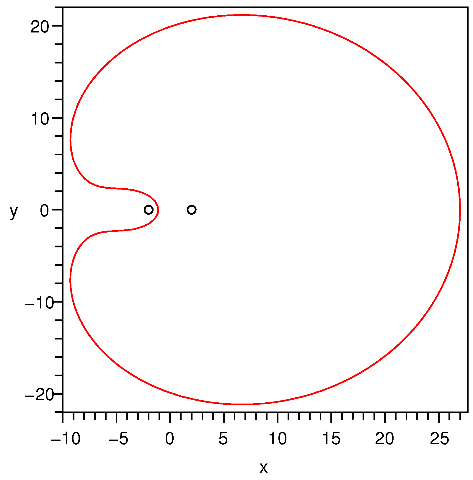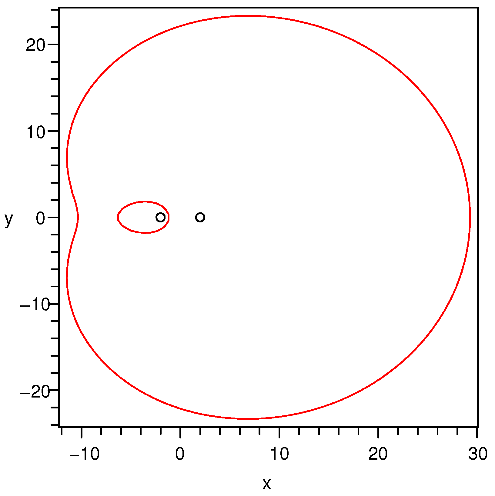Let us check it by numerical experiments. By setting $(x_p,y_p)=(-2,0)$, $(x_p^{\prime },y_p^{\prime })=(2,0)$, $ϵ=1.5$, ${ϵ}^{\prime }=2.5$, we plot graphs of the criterion curves for $\lambda =0.05,0.046487,0.045$ respectively in Figure 1, Figure 2 and Figure 3. The reason why $\lambda$ selects these three values is that, under the given parameter setting, $\lambda =0.046487$ is found numerically at a critical point corresponding to the critical curve among the other two kinds of curves. Thus, the other two values $0.05$ and $0.045$ from both sides of the critical value are chosen to show the bifurcation phenomenon.

The latter case will be analyzed extensively in the next subsection, so we just summarize the case $ϵ\ne {ϵ}^{\prime }$ below.

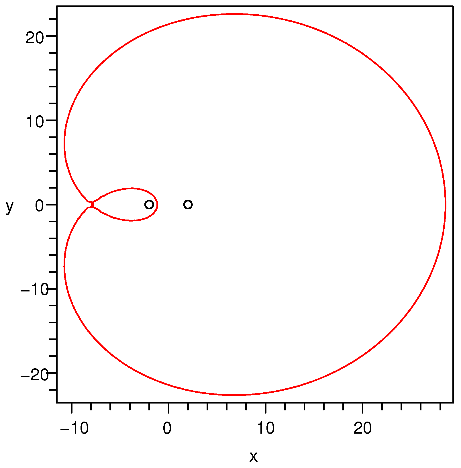
Proposition 2.

For $ϵ\ne {ϵ}^{\prime }$, the criterion curves defined by Equation (11) can be divided into 3 kinds of curves according to the number of intersecting points of a criterion curve and the straight line determined by the two points $(x_p,y_p)$ and $(x_p^{\prime },y_p^{\prime })$, i.e., the number of roots of Equation (14). Specifically, the three cases are as follows:

(a) 

If the number is 2, the curve is a closed connected curve. A typical graph of this case is shown in Figure 1;

(b) 

If the number is 3, the curve is a closed connected curve. A typical graph of this case is shown in Figure 2;

(c) 

If the number is 4, the curve is two separated curves. A typical graph of this case is shown in Figure 3.

3.2. Qualities of the Criterion Curve if $ϵ$ Is Known

If the path-loss exponent $ϵ$ is known, i.e., in this case, the ML estimation is proposed for $(s_p,x_p,y_p)$ as in [10], by a similar reasoning process, we have the criterion curve as

$$\begin{array}{c}\hfill \sqrt{{(x-x_p)}^2+{(y-y_p)}^2}=\lambda \sqrt{{(x-x_p^{\prime })}^2+{(y-y_p^{\prime })}^2}\end{array}$$

(15)

with given parameters $\lambda ={10}^{\frac{1}{10ϵ}(s_p-s_p^{\prime })}>0$, $(x_p,y_p)$ and $(x_p^{\prime },y_p^{\prime })$.

Clearly, the curve is a straight line when $\lambda =1$, and a circle when $\lambda \ne 1$. Though these basic facts have been discovered in [10], we describe some more general and deeper qualities in the following propositions.

Proposition 3.

When $\lambda \ne 1$, the circle defined by Label (15) is centered at

$$\begin{array}{c}\hfill \left(\frac{x_p-{\lambda }^2{x}_p^{\prime }}{1-{\lambda }^2},\frac{y_p-{\lambda }^2{y}_p^{\prime }}{1-{\lambda }^2}\right)\end{array}$$

(16)

with radius $\frac{\lambda }{|1-{\lambda }^2|}\sqrt{{(x_p-x_p^{\prime })}^2+{(y_p-y_p^{\prime })}^2}$, i.e., $\frac{\lambda }{|1-{\lambda }^2|}$ times the distance between $(x_p,y_p)$ and $(x_p^{\prime },y_p^{\prime })$. While $\lambda =1$, the straight line defined by (15) is perpendicular to the line connecting $(x_p,y_p)$ and $(x_p^{\prime },y_p^{\prime })$ and containing their midpoint.

In the circle case, the radius tends to infinity when $\lambda$ tends to 1, which also means the circle turns out to be a straight line.

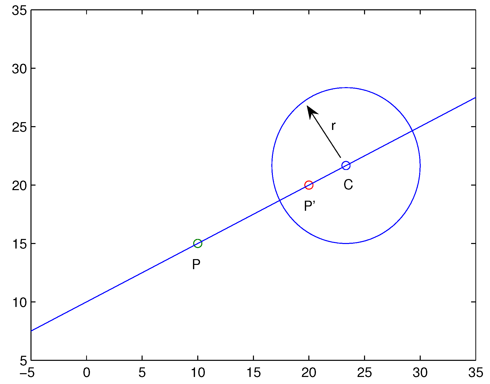
With $s_p$ and $P\stackrel{\Delta }{=}(x_p,y_p)$ fixed, an important topic is checking whether a given circle is a criterion curve, and, if it is, how we can find the corresponding $P^{\prime }\stackrel{\Delta }{=}(x_p^{\prime },y_p^{\prime })$. As shown in Figure 4, given the point P and a circle centered at C with radius r, it is important to figure out whether the circle is a criterion curve, and what $P^{\prime }$ is at this moment.

Let us change the Formula (16) into a vector form:

$$\begin{array}{c}\hfill \overrightarrow{C}=\frac{\overrightarrow{P}-{\lambda }^2\overrightarrow{P^{\prime }}}{1-{\lambda }^2}.\end{array}$$

(17)

Thus, we have

$$\begin{array}{c}\hfill \overrightarrow{P^{\prime }}=\frac{\overrightarrow{P}+({\lambda }^2-1)\overrightarrow{C}}{{\lambda }^2}.\end{array}$$

(18)

Hence, $P^{\prime }$, shown in Figure 4, can be calculated from (18) directly if $\lambda$, P and C are known.

Let us deduce a formula to calculate $\lambda$ from given information: points P and C, and circle radius r. In the case of $\lambda >1$, shown in Figure 4, by the aforementioned fact, it follows that

$$\begin{array}{c}\hfill r=\frac{\lambda }{|1-{\lambda }^2|}|P{P}^{\prime }|\end{array}$$

(19)

and

$$\begin{array}{c}\hfill |P{P}^{\prime }|=\frac{|{\lambda }^2-1|}{{\lambda }^2}|PC|,\end{array}$$

(20)

derived by (17). Thus, from (19) and (20), we derive

$$\begin{array}{c}\hfill r=\frac{1}{\lambda }|PC|,\end{array}$$

(21)

and thus

$$\begin{array}{c}\hfill \lambda =\frac{|PC|}{r}.\end{array}$$

(22)

Similar results can be derived in the case $0<\lambda <1$.

Therefore, now we can calculate $P^{\prime }$ by Formulas (18) to (22) when $\lambda \ne 1$, i.e., $r\ne |PC|$. In the case $\lambda =1$, or $r=|PC|$, we know that the corresponding curve should be a straight line rather a circle. Thus, if a given circle contains the point P, it is impossible to be a criterion curve. Let us summarize these facts as a proposition below.

Proposition 4.

Assuming points $P=(x_p,y_p)$ and $C=(x_c,y_c)$, and a circle centered at C with radius $r>0$ are given, then the following assertions hold:

(i) If the circle contains point P, i.e., $r=|PC|$, then the circle is not a criterion curve. Moreover, a straight line traversing through P is not a criterion curve.

(ii) If $r\ne |PC|$, then the circle is a criterion curve, and the corresponding $P^{\prime }=(x_p^{\prime },y_p^{\prime })$ in (15) can be calculated as:

$$\begin{array}{c}\hfill \overrightarrow{P^{\prime }}=\frac{\overrightarrow{P}+({\lambda }^2-1)\overrightarrow{C}}{{\lambda }^2}\end{array}$$

(23)

with $\lambda =|PC|/r$.

Another obvious fact is that, under case (ii) of Proposition 4, the circle contains either one of P and $P^{\prime }$, and the other is out of the circle, as shown in Figure 4. This also serves as an explanation as to why it fails to be a criterion curve if a circle contains P itself. Moreover, three noncollinear points are not located in any criterion curve, if the circle determined by the three points contains P.

4. Consistence Condition for ML Estimation of Transmitter Power

In this section, we deduce the consistence condition to guarantee convergence of the ML estimate for $\theta$, i.e., ${\theta }_n\to \theta$ as $n\to \infty$. Roughly speaking, the consistence condition is that the location set $\left\{(x_i,y_i)\right\}$ should be rich enough in some sense. A criterion is given and proved.

Let us introduce the definition for consistence condition, which is a requirement for richness of the locations $\left\{(x_i,y_i)\right\}$, as introduced in the former section. The requirement is somewhat similar to `persistence of excitation condition’ in a least squares algorithm to guarantee the convergence.

Let us introduce a limit set of a sequence of point sets in terms of standard Euclidean distance.

Definition 1.

Denote a series of nonintersecting and successive index sets for the whole natural numbers as $\{A_j,j=1,2,\dots \}$ with $|A_j|\le m$. Let $S_k=\{P_i\in R^n,i\in A_k\}$ is a point set in $R^n$. A point $P\in R^n$ is called a limit point of the sequence of point sets $\left\{S_k\right\}$, if for $\forall \epsilon >0$, there exists $j_0>0$ and $i_j\in A_j$ such that

$$|P_{i_j}-P|<\epsilon$$

holds for $j>j_0$. The set comprised of all such limit points is called the limit set of the set sequence $\left\{S_k\right\}$, denoted as $Lim\left(S_k\right)$.

For example, letting

$$S_k=\left\{\frac{1}{k},-1-\frac{1}{k^2},1+e^{-k}\right\},$$

we have its limit set to $Lim\left(S_k\right)=\{0,-1,1\}$.

Below we define the criterion curve strictly, which actually has been introduced in Section 3.

Definition 2.

A criterion curve is defined by equation of $x,y$ as

$$\begin{array}{c}\hfill {\left[{(x-x_p)}^2+{(y-y_p)}^2\right]}^{ϵ/2}=\lambda {\left[{(x-x_p^{\prime })}^2+{(y-y_p^{\prime })}^2\right]}^{{ϵ}^{\prime }/2}\end{array}$$

(24)

with given parameters $\lambda ={10}^{\frac{1}{10}(s_p-s_p^{\prime })}>0$, $(ϵ,x_p,y_p)$ and $({ϵ}^{\prime },x_p^{\prime },y_p^{\prime })$.

Remark 1.

When $ϵ={ϵ}^{\prime }$, a criterion curve is a circle for if $\lambda \ne 1$ and a line if $\lambda =1$, as already shown in Section 3. Thus, under this setting, four noncollinear and nonconcyclic points are impossible to locate in any single criterion curve.

Now, we are in a position to state a consistence result for ML estimation for transmitter power model.

Theorem 1.

Suppose that the location set ${\{x_i,y_i\}}_1^{\infty }$ is in a bounded region, and denote

$$\begin{array}{c}\hfill S_k\stackrel{\Delta }{=}\{(x_{km+i},y_{km+i}),i=1,\dots ,m\},\end{array}$$

(25)

where $m\ge 3$ is a positive integer. If the limit set $Lim\left(S_k\right)$ does not locate in any single criterion curve given by (24), then the ML estimation for model (2) with likelihood function given by (5) is very consistent, i.e., the estimates converge to the true vale with probability 1 as the data number tends to infinity.

Proof. 

Theorem 3 is used to prove the above theorem. Since the model is assumed to be located in a local region, we need only to check the two conditions therein. By the likelihood function given by (5) and density for $s_i$ given by (4), we have

$$\begin{array}{c}\frac{\partial \sqrt{f}}{\partial s_p}=\frac{\sqrt{f}(s_p-s_i-10ϵ{log}_{10}{d}_{ip})}{2{\sigma }^2},\hfill \\ \frac{\partial \sqrt{f}}{\partial ϵ}=-\frac{\partial \sqrt{f}}{\partial s_p}·10{log}_{10}{d}_{ip},\hfill \\ \frac{\partial \sqrt{f}}{\partial x_p}=-\frac{\partial \sqrt{f}}{\partial s_p}·\frac{10ϵ(x_p-x_i)}{d_{ip}^{2}log10},\hfill \\ \frac{\partial \sqrt{f}}{\partial y_p}=-\frac{\partial \sqrt{f}}{\partial s_p}·\frac{10ϵ(y_p-x_i)}{d_{ip}^{2}log10},\hfill \end{array}$$

where $\sqrt{f}$ used on the right-hand side is used to make the expressions brief. By the fact that all parameters belong to a compact set, the condition (ii) of Theorem 3 is satisfied.

The continuity of $\sqrt{f}$ with respect to all variables is obvious. By Remark 5, we need only to verify (53). To show (53) for density (4), it is sufficient to show that, for any different $\theta$ and ${\theta }^{\prime }$, there exist s and $(x,y)\in Lim\left(S_k\right)$ such that

$$\begin{array}{c}\hfill f(s;x,y,\theta )\ne f(s;x,y,{\theta }^{\prime }).\end{array}$$

(26)

By substituting (4) to (26), we have

$$\begin{array}{c}\hfill {\left[{(x-x_p)}^2+{(y-y_p)}^2\right]}^{ϵ/2}\ne \lambda {\left[{(x-x_p^{\prime })}^2+{(y-y_p^{\prime })}^2\right]}^{{ϵ}^{\prime }/2},\end{array}$$

(27)

which means that there is no criterion curve containing all points of the limit set $Lim\left(S_k\right)$. In other words, this is equivalent to say that the limit set $Lim\left(S_k\right)$ is not located in any single criterion curve given by (24), which finishes the proof of the theorem. ☐

Based on Theorem 1, the ML estimate for transmitter power may fail even if the number of observation tends to infinity if the whole location set ${\{x_i,y_i\}}_1^{\infty }$ belongs to a single criterion curve. Below are two typical cases when $ϵ$ is known.

(i). The set ${\{x_i,y_i\}}_1^{\infty }$ is located in a straight line, which means $\lambda =1$ and $ϵ={ϵ}^{\prime }$ in (24). In this case, the ML estimator for location $(x_p,y_p)$ may tend to its symmetrical point with respect to the line yet the estimate for $s_p$ still works, as in Example 2. Furthermore, if the set ${\{x_i,y_i\}}_1^{\infty }$ is asymptotically located in a straight line, the same phenomenon happens, as shown in Example 4.

(ii). The set ${\{x_i,y_i\}}_1^{\infty }$ is located in a circle, which means $\lambda \ne 1$ and $ϵ={ϵ}^{\prime }$ in (24). In this case, the ML estimate may tend to another location $L_p^{\prime }=(x_p^{\prime },y_p^{\prime })$ given by (23), and estimate for $s_p$ tends to $s_p^{\prime }$, as in Example 3.

However, even in the two cases above, it is still possible to see that the ML estimators converge to the true value because the true value are also the solution of the likelihood function.

5. Numerical Algorithm and Experiments

Let us first develop a recursive numerical algorithm to minimize $M_n\left(\theta \right)$ in (6) by using Matlab code/fminsearch/. When the n-th ML estimate for $\theta$ is numerically found to be ${\theta }_n$, the next minima ${\theta }_{n+1}$ for $M_{n+1}\left(\theta \right)$ is numerically searched based on ${\theta }_n$ as:

$${\theta }_{n+1}=\mathrm{fminsearch}(@M_{n+1},{\theta }_n).$$

This means the starting point of the next search is ${\theta }_n$, rather than any other randomly selected value. Thus, the information obtained by the former step has been used for the next search, which may increase the effectiveness.

For simplicity, the numerical experiments below are designed to investigate the performance of ML estimation for parameters $s_p,x_p,y_p$, instead of $\theta =(ϵ,s_p,x_p,y_p)$. Naturally, similar phenomena exist for ML estimation of $\theta$. Four numerical experiments below are designed to investigate the asymptotical performances of the ML estimation for $(s_p,x_p,y_p)$ in model (2) as the observation number tends to infinity. The first one achieved a successful observation while the rest three failed. The essential reason for the failure is that the likelihood function (5), or the equivalent function $M_n(·,·,·)$ in (6), has multiple roots when some conditions are not met. Note that, even in the three examples of failure, the ML estimation may still work since the true value is also a root of the likelihood function. It depends on the numerical algorithm to find the roots of the likelihood function.

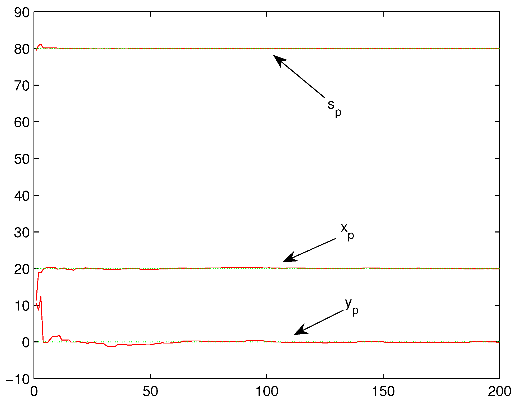
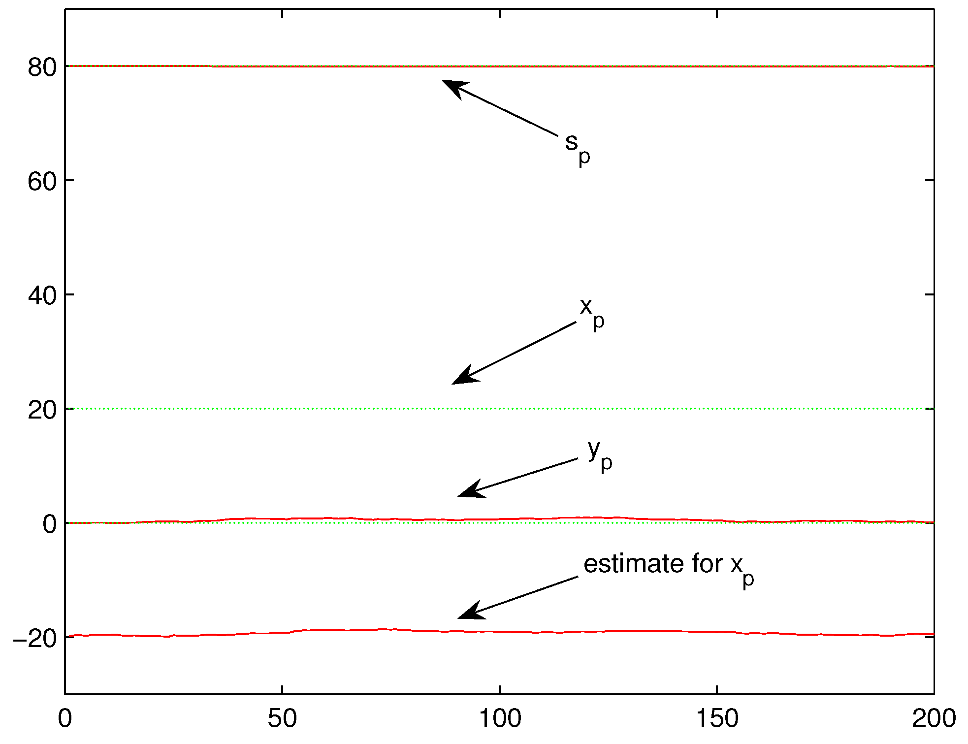
Example 1.

Let $ϵ=1$, $x_p=20,y_p=0,s_p=80$ in (2) and (3), $w_i\sim \mathcal{N}(0,{0.5}^2)$, and assume all locations $(x_i,y_i)$ are all located in the set $\left\{\right(0,0),(40,0),(0,-20),(0,20\left)\right\}$ successively infinite times. The performance has been shown in Figure 5.

Clearly, the corresponding location set $S_k$ in Theorem 1 is:

$$S_k=\{(0,0),(40,0),(0,-20),(0,20)\}.$$

Hence, $Lim\left(S_k\right)$ is still comprised of these four noncollinear and nonconcyclic points. By Theorem 1 and Remark 1, the ML estimation for $(s_p,x_p,y_p)$ will definitely converge to all true values as shown in Figure 5, which coincides with the numerical experiments.

The set $S_k$ does not need to own four noncollinear and nonconcyclic points. As a matter of fact, $A_k$ consists of three noncollinear points (or three collinear points) may still work.

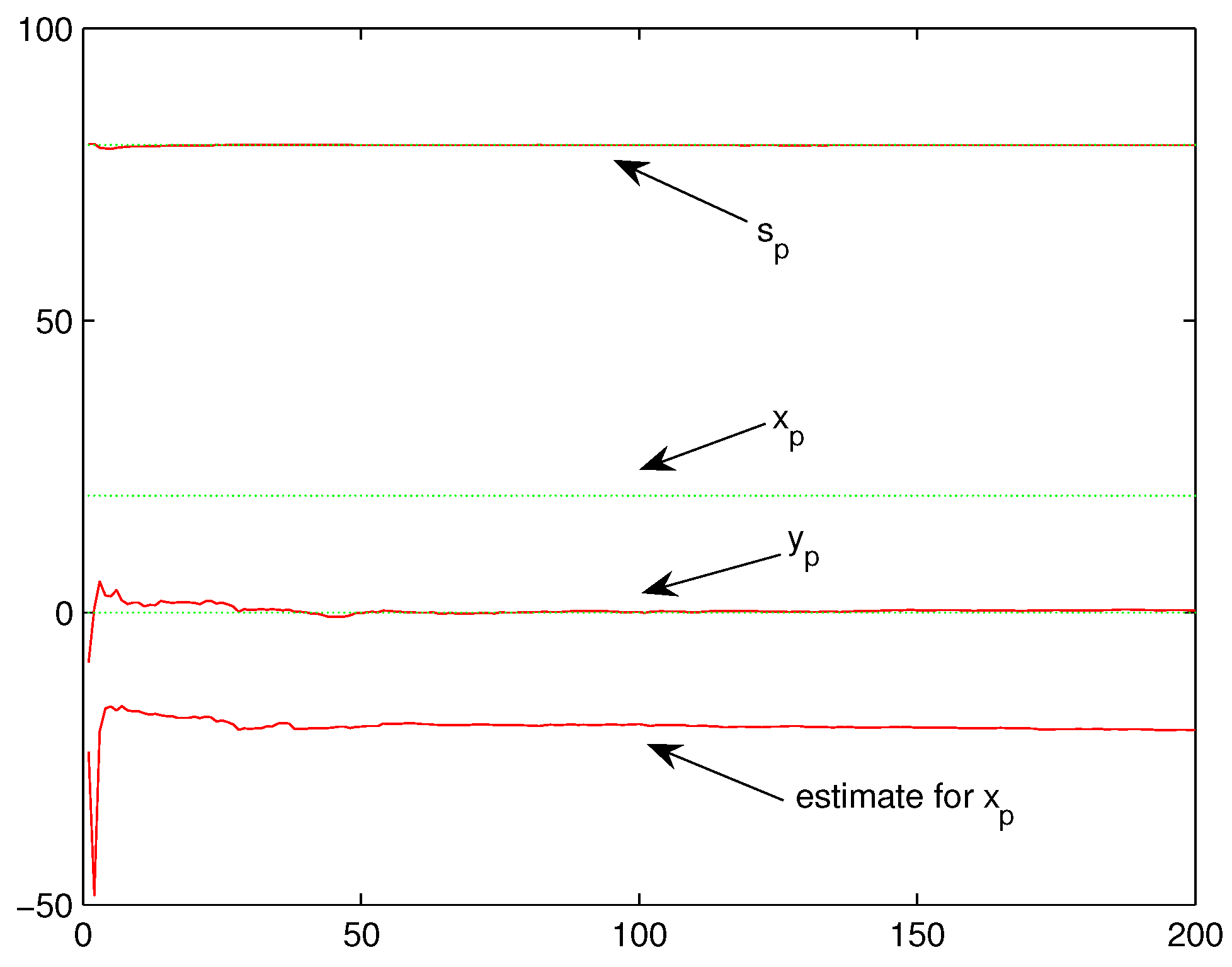
Example 2.

Under the same setting of Example 1, expect that all locations $(x_i,y_i)$ are located in the set $\left\{\right(x,y)\text{:}x=0,y\in [-100,100\left]\right\}$. The performance has been shown in Figure 6.

The location set $\{(x_i,y_i),i=1,2,\dots \}$ is obviously located in a criterion curve, since they are all located in the straight line $x=0$. The corresponding $P^{\prime }=(x_p^{\prime },y_p^{\prime })=(-20,0)$ in (15) by the fact $P=(20,0)$. In addition, the corresponding $\lambda =1$ under this case, so, by (10), $s_p^{\prime }=s_p$. This means that the ML estimates for $s_p$ and $y_p$ have no bias, while the ML estimate for $x_p$ may tend to $x_p^{\prime }$, which has been discovered by the experiment. By observing that the symmetric point of $(20,0)$ with respect to the line $x=0$ is $(-20,0)$, the ML estimators for $x_p$ may converge to $-20$, yet the estimators for $y_p$ and $s_p$ still work, as shown in Figure 6.

Example 3.

Under the same setting of Example 1, expect that all locations $(x_i,y_i)$ are located in the set

$$\{(x,y):\sqrt{{(x-20)}^2+y^2}=\lambda \sqrt{{(x+20)}^2+y^2}\}$$

with $\lambda =10$. The performance has been shown in Figure 7.

The location set $\{(x_i,y_i),i=1,2,\dots \}$ in Example 3 is also located in a criterion curve, since they are all located in the same circle with center $(-2020/99,0)$ with radius $r=400/99$, calculated by Proposition 4. The corresponding $P^{\prime }=(-20,0)$ in (15) and the corresponding $\lambda =10$, so, by (10), $s_p^{\prime }=70$. This means that ML estimate for $y_p$ have no bias, while ML estimates for $x_p$ and $s_p$ may tend to $x_p^{\prime }$ and $s_p^{\prime }$ respectively, which has been discovered by the experiment, as shown in Figure 7.

Example 4.

Under the same setting of Example 1, expect all locations $\{(x_i,y_i)\text{:}{x}_i=\frac{1}{i+10000},y_i\in [-100,100]\}$. The performance has been shown in Figure 8.

Note that the corresponding location set $S_k$ in Theorem 1 is:

$$S_k=\left\{\left(\frac{1}{10000+4k+i},y\right),y\in [-100,100],i=1,2,3,4\right\}.$$

Clearly, $Lim\left(S_k\right)$ is located on line $x=0$. Thus, it is located on a single criterion curve. A similar phenomenon of Example 2 happens. By observing that the symmetric point of $(20,0)$ with respect to the line $x=0$ is $(-20,0)$, the ML estimators for $x_p$ may converge to $-20$ yet the estimators for $y_p$ and $s_p$ still work, as shown in Figure 8.

It is similar to design a set of numerical experiments to make the ML estimations for $\theta =(ϵ,s_p,x_p,y_p)$ all fail. The four simple examples above are just used to demonstrate some basic features of the proposed ML estimate algorithm.

6. Consistence Analysis of Maximum Likelihood Estimation

This section serves as theoretical preliminaries for the former mathematical analysis, which contains general consistence analysis for the proposed ML estimation algorithm based on independent observations with different distributions. As for independent identically distributed observation cases, we refer to Theorem 1.3.3 in Chapter 1 of book [15]. Hence, Theorem 2 here can be taken as an extension of the counterpart in [15]. Furthermore, we propose an easy way of checking the criterion in the following Theorem 3. On the other hand, the readers who are more concerned with practical applications are suggested to pay more attention to Theorem 3.

Although the ML method, suggested by R. A. Fisher, has attracted the interest of mathematicians in theoretical performance analysis for a long time, there are still remain open quite basic issues such as the one investigated in this paper. Thus, this section investigates the basic strong consistence for theoretical preparation.

Let $(\mathcal{X},\mathcal{U},P_{\theta },\Theta )$ be a statistical experiment, which means that $(\mathcal{X},\mathcal{U},P_{\theta })$ is a probability space for any $\theta \in \Theta$. Let $P_{\theta }$ be absolutely continuous with respect to measure $\mu$ on $\mathcal{U}$ and thus $\frac{d{P}_{\theta }}{d\mu }=p(X,\theta )$, i.e., something like density function. Let X be the observation data generated by a certain statistical experiment. Thus, the function $p(X,\theta )$ can be taken as a likelihood function corresponding to the experiment and observation X. The statistic $\widehat{\theta }$ defined by

$$\begin{array}{c}\hfill \widehat{\theta }=arg\underset{\theta \in \Theta }{sup}p(X,\theta )\end{array}$$

(28)

is called the ML estimator for the parameter $\theta$ based on the observation X. In the case of independent identically distributed (iid) observations, $X_1,\dots ,X_n$, where $X_i$ possesses the density $f(x,\theta )$ with respect to measure $\mu$. The ML estimator ${\widehat{\theta }}_n$ has a simple form as

$$\begin{array}{c}\hfill {\widehat{\theta }}_n=arg\underset{\theta \in \Theta }{sup}\prod _{i=1}^{n}f(X_i,\theta ).\end{array}$$

(29)

Moreover, in many applications, the likelihood function depends on some other varying quantities, e.g., the likelihood function for transmitter power model by (5) involves $s_i$ and $(x_i,y_i)$. This means that the ML estimator ${\widehat{\theta }}_n$ is generally

$$\begin{array}{c}\hfill {\widehat{\theta }}_n=arg\underset{\theta \in \Theta }{sup}\prod _{i=1}^{n}f(X_i,{\overline{\theta }}_i,\theta ),\end{array}$$

(30)

where ${\overline{\theta }}_i$ is a deterministic quantity (or vector), e.g., ${\overline{\theta }}_i={[s_i,x_i,y_i]}^T$ in (5). The issue to be faced now is to estimate parameter $\theta$ via the available observations and the varying data $\left\{{\overline{\theta }}_i\right\}$. Naturally, some restrictions upon the extra data set $\left\{{\overline{\theta }}_i\right\}$ are required to guarantee the consistence.

In the aforementioned iid case with likelihood function (29), the ML estimator ${\widehat{\theta }}_n$ is strongly consistent (see Theorem 1.3.3 in Chapter 1 of book [15]), i.e., ${\widehat{\theta }}_n\to \theta$ with probability 1 as $n\to \infty$. Below, we intend to obtain a similar result by using the case with likelihood function as (30).

Theorem 2.

Let Θ be a bounded closed set in ${\mathcal{R}}^k$, $f(x,{\overline{\theta }}_i,\theta )$ be a continuous function of $\theta \in \Theta$ for almost all $x\in \mathcal{X}$, $i=1,2,\dots$. Let the following conditions be fulfilled with a real number $q\ge 2$:

(i) Denote a series of nonintersecting and successive index sets for the whole natural numbers as $\{A_j,j=1,2,\dots \}$ with the volume of $A_j$ less than or equal to a constant positive integer m. For all $\theta \in \Theta$ and all $\gamma >0$, there exists a positive number ${\kappa }_{\theta }\left(\gamma \right)$ (may depend on θ, q and γ) such that

$$\begin{array}{cc}\hfill \underset{j}{inf}\underset{i\in A_j}{max}& \underset{|\theta -{\theta }^{\prime }|>\gamma }{inf}{\int }_{\mathcal{X}}{\left|f^{\frac{1}{q}}(x,{\overline{\theta }}_i,\theta )-f^{\frac{1}{q}}(x,{\overline{\theta }}_i,{\theta }^{\prime })\right|}^{q}d\mu \hfill \\ & \ge {\kappa }_{\theta }\left(\gamma \right)>0.\hfill \end{array}$$

(31)

(ii) For any ${\overline{\theta }}_i$, $\delta >0$ and $\theta \in \Theta$, there exists a positive number ${\omega }_{\theta }\left(\delta \right)$ (may depend on θ, q and δ) such that

$$\begin{array}{c}{\left({\int }_{\mathcal{X}}\underset{|h|\le \delta }{sup}{\left|f^{\frac{1}{q}}(x,{\overline{\theta }}_i,\theta )-f^{\frac{1}{q}}(x,{\overline{\theta }}_i,\theta +h)\right|}^{q}d\mu \right)}^{\frac{1}{q}}\hfill \\ \le {\omega }_{\theta }\left(\delta \right)\underset{\delta \to 0}{\to }0.\hfill \end{array}$$

(32)

Then, for any fixed $\theta \in \Theta$, the ML estimator ${\widehat{\theta }}_n$ given by (30) tends to θ as $n\to \infty$ with probability 1.

Let us explain the two conditions briefly here. The condition (i) requires that in any index set $A_j$ there is at least a density function with a different value as $\theta$ is changed. This means the data set $\{{\overline{\theta }}_i,i\in A_j\}$ should be rich enough to make density function $f(x,{\overline{\theta }}_i,\theta )$ distinguishable according to different values of $\theta$. On the other hand, condition (ii) desires that the density function has certain continuity with respect to $\theta$ in some sense.

Remark 2.

This theorem is a twofold extension of Theorem 4.3 in Chapter 1 of book [15]. Firstly, the theorem in book [15] deals with an iid likelihood function as (29), which is just a special case of (30) without ${\overline{\theta }}_i$ in the likelihood function. Secondly, a parameter q is introduced here in the conditions (i) and (ii) to include the counterpart conditions therein as a special case of $q=2$, although, $q=2$ is a wise choice.

Remark 3.

When we consider a fixed true value ${\theta }_0$, the condition (i) can be reduced to ${\kappa }_{{\theta }_0}\left(\gamma \right)>0$. This means only the difference between (any) ${\theta }^{\prime }$ and (fixed) ${\theta }_0$ is required with $|{\theta }^{\prime }-{\theta }_0|>\gamma$.

Before prove the theorem, let us introduce an extension of Young’s inequality [16] below and refer its proof to [17].

Lemma 1.

Suppose that $a\ge 0,b\ge 0$, and $\frac{1}{p}+\frac{1}{q}=1$ with $1<p\le 2\le q$. Then,

$$\begin{array}{c}\hfill \frac{1}{q}{\left|a^{\frac{1}{q}}-b^{\frac{1}{q}}\right|}^q\le \frac{1}{p}a+\frac{1}{q}b-a^{\frac{1}{p}}{b}^{\frac{1}{q}}\le \frac{1}{p}{\left|a^{\frac{1}{p}}-b^{\frac{1}{p}}\right|}^p,\end{array}$$

(33)

where the equalities hold if $p=q=2$ or $a=b$.

Remark 4.

This lemma develops an extension of the classic Young’s inequality; see, e.g., [16],

$$a^{\frac{1}{p}}{b}^{\frac{1}{q}}\le \frac{1}{p}a+\frac{1}{q}b$$

for $a\ge 0,b\ge 0$, and $\frac{1}{p}+\frac{1}{q}=1$ with $p>0,q>0$, which is a source of lots of important inequalities, e.g., Holder’s inequality and Minkowski’s inequality. A corollary from the proof is

$$\begin{array}{c}\hfill {\left|a^{\frac{1}{q}}-b^{\frac{1}{q}}\right|}^q\le {\left|a^{\frac{1}{p}}-b^{\frac{1}{p}}\right|}^p.\end{array}$$

(34)

The below proof for Theorem 2 shares the main ideas of the counterpart for Theorem 4.3 in [15].

Proof of Theorem 2.

Denote

$$\begin{array}{c}\hfill {\Pi }_n\left(u\right)=\prod _{j=1}^n\prod _{i\in A_j}\frac{f(x_i,{\overline{\theta }}_i,\theta +u)}{f(x_i,{\overline{\theta }}_i,\theta )}.\end{array}$$

(35)

Notice that the maximum operator is taking over a finite set $A_j$ in (31) of condition (i), thus there exists an index $i_j\in A_j$ such that

$$\begin{array}{c}\hfill \underset{|\theta -{\theta }^{\prime }|>\gamma }{inf}{\int }_{\mathcal{X}}{\left|f^{\frac{1}{q}}(x,{\overline{\theta }}_{i_j},\theta )-f^{\frac{1}{q}}(x,{\overline{\theta }}_{i_j},{\theta }^{\prime })\right|}^{q}d\mu \ge {\kappa }_{\theta }\left(\gamma \right)>0.\end{array}$$

(36)

Let $\Gamma$ be a sphere of a small radius $\delta$ located entirely in the region $|u|>\frac{1}{2}\gamma$. We shall estimate first $E{sup}_{\Gamma }{\Pi }_n{\left(u\right)}^{\frac{1}{q}}$. Supposing that $u_0$ is the center of $\Gamma$, then

$$\begin{array}{cc}\hfill \underset{u\in \Gamma }{sup}{\Pi }_n{\left(u\right)}^{\frac{1}{q}}& =\underset{u\in \Gamma }{sup}\prod _{j=1}^n\prod _{i\in A_j}{\left(\frac{f(x_i,{\overline{\theta }}_i,\theta +u)}{f(x_i,{\overline{\theta }}_i,\theta )}\right)}^{\frac{1}{q}}\hfill \\ & \le \prod _{j=1}^n\prod _{i\in A_j}{f}^{-\frac{1}{q}}(x_i,{\overline{\theta }}_i,\theta )[f^{\frac{1}{q}}(x_i,{\overline{\theta }}_i,\theta +u_0)\hfill \\ & +\underset{|h|\le \delta }{sup}\left|f^{\frac{1}{q}}(x_i,{\overline{\theta }}_i,\theta +u_0+h)-f^{\frac{1}{q}}(x_i,{\overline{\theta }}_i,\theta +u_0)\right|]\hfill \\ & \stackrel{\Delta }{=}\prod _{j=1}^n\prod _{i\in A_j}{\overline{f}}_i.\hfill \end{array}$$

(37)

We now intend to find a suitable upper bound for the expectation of the left-hand side of (37). This can be done by considering the right-hand side in two separated nonintersecting index subsets of i, denoted by $A^{\prime }\stackrel{\Delta }{=}\{i_j,j=1,2,\dots ,n\}$ and $A^{″}\stackrel{\Delta }{=}{\bigcup }_{j=1}^n{A}_j-A^{\prime }$. By taking expectation over index set $A^{\prime }$ for (37), we have

$$\begin{array}{cc}\hfill E\prod _{i\in A^{\prime }}{\overline{f}}_i& \le ({\int }_{\mathcal{X}}{f}^{\frac{1}{p}}(x,{\overline{\theta }}_i,\theta )f^{\frac{1}{q}}(x,{\overline{\theta }}_i,\theta +u_0)d\mu \hfill \\ & +{\int }_{\mathcal{X}}\underset{|h|\le \delta }{sup}\left|f^{\frac{1}{q}}(x,{\overline{\theta }}_i,\theta +u_0+h)-f^{\frac{1}{q}}(x,{\overline{\theta }}_i,\theta +u_0)\right|\hfill \\ & ·f^{\frac{1}{p}}(x,{\overline{\theta }}_i,\theta )d\mu {)}^n.\hfill \end{array}$$

(38)

Here and hereafter, p satisfies $\frac{1}{p}+\frac{1}{q}=1$. By Lemma 1 and (36), the first term of (38) derives

$$\begin{array}{c}{\int }_{\mathcal{X}}{f}^{\frac{1}{p}}(x,{\overline{\theta }}_i,\theta )f^{\frac{1}{q}}(x,{\overline{\theta }}_i,\theta +u_0)d\mu \hfill \\ \le {\int }_{\mathcal{X}}[\frac{1}{p}f(x,{\overline{\theta }}_i,\theta )+\frac{1}{q}f(x,{\overline{\theta }}_i,\theta +u_0)\hfill \\ -\frac{1}{q}{\left|f^{\frac{1}{q}}(x,{\overline{\theta }}_i,\theta )-f^{\frac{1}{q}}(x,{\overline{\theta }}_i,\theta +u_0)\right|}^q]d\mu \hfill \\ \le 1-\frac{1}{q}{\kappa }_{\theta }\left(\frac{\gamma }{2}\right).\hfill \end{array}$$

(39)

By Hölder’s inequality, the second term of (38) derives

$$\begin{array}{c}{\int }_{\mathcal{X}}\underset{|h|\le \delta }{sup}\left|f^{\frac{1}{q}}(x,{\overline{\theta }}_i,\theta +u_0+h)-f^{\frac{1}{q}}(x,{\overline{\theta }}_i,\theta +u_0)\right|f^{\frac{1}{p}}(x,{\overline{\theta }}_i,\theta )d\mu \hfill \\ \le {\omega }_{\theta +u_0}\left(\delta \right).\hfill \end{array}$$

(40)

By the inequality $1+x\le e^x$ and (38)–(40), we obtain

$$\begin{array}{c}\hfill E\prod _{i\in A^{\prime }}{\overline{f}}_i\le exp\left\{-n\left(\frac{1}{q}{\kappa }_{\theta }\left(\frac{\gamma }{2}\right)-{\omega }_{\theta +u_0}\left(\delta \right)\right)\right\}.\end{array}$$

(41)

By taking expectation over index set $A^{″}$ for (37), we have

$$\begin{array}{cc}\hfill E\prod _{i\in A^{″}}{\overline{f}}_i& \le ({\int }_{\mathcal{X}}{f}^{\frac{1}{p}}(x,{\overline{\theta }}_i,\theta )f^{\frac{1}{q}}(x,{\overline{\theta }}_i,\theta +u_0)d\mu \hfill \\ & +{\int }_{\mathcal{X}}\underset{|h|\le \delta }{sup}\left|f^{\frac{1}{q}}(x,{\overline{\theta }}_i,\theta +u_0+h)-f^{\frac{1}{q}}(x,{\overline{\theta }}_i,\theta +u_0)\right|\hfill \\ & ·f^{\frac{1}{p}}(x,{\overline{\theta }}_i,\theta )d\mu {)}^{n(m-1)}.\hfill \end{array}$$

(42)

By Hölder’s inequality, the first term of (42) is not greater than 1, and the second term of (42) satisfies inequality (40). Similar to (41), we obtain

$$\begin{array}{c}\hfill E\prod _{i\in A^{″}}{\overline{f}}_i\le exp\left\{n(m-1){\omega }_{\theta +u_0}\left(\delta \right)\right\}.\end{array}$$

(43)

Finally, by (41) and (43), we have

$$\begin{array}{c}\hfill E\underset{u\in \Gamma }{sup}{\Pi }_n^{\frac{1}{q}}\left(u\right)\le exp\left\{-n\left(\frac{1}{q}{\kappa }_{\theta }\left(\frac{\gamma }{2}\right)-m{\omega }_{\theta +u_0}\left(\delta \right)\right)\right\}.\end{array}$$

(44)

By definition of ${\omega }_{\theta }\left(\delta \right)$ in (32), it is easy to show that, e.g., see [15],

$$\begin{array}{c}\hfill \underset{\delta \to 0}{lim}\underset{\theta \in \Theta }{sup}{\omega }_{\theta }\left(\delta \right)=0.\end{array}$$

(45)

Noticing the fact m is a constant integer, this means

$$\begin{array}{c}\hfill \frac{1}{q}{\kappa }_{\theta }\left(\frac{\gamma }{2}\right)-m{\omega }_{\theta +u_0}\left(\delta \right)>0\end{array}$$

(46)

can be held if we select sufficiently small $\delta$. Thus, the right-hand side of (44) tends exponentially to 0 as $n\to \infty$.

Fix $\gamma >0$ and cover the exterior of the sphere $|u|\le \gamma$ by M spheres ${\Gamma }_j,j=1,\dots ,M$, of radius $\delta$ with centers $u_j$. The number $\delta$ is chosen to be sufficiently small so that all the spheres will be located in the region $|u|>\frac{1}{2}\gamma$ and so that, for all j, the inequality $m{\omega }_{\theta +u_j}\left(\delta \right)\le \frac{1}{2q}{\kappa }_{\theta }\left(\frac{1}{2}\gamma \right)$ satisfied. Then, by definition of ${\Pi }_n$ and (44),

$$\begin{array}{cc}\hfill P\{|{\widehat{\theta }}_n-\theta |>\gamma \}& \le \sum _{i=1}^{M}P\{|{\widehat{\theta }}_n-\theta |\in {\Gamma }_i\}\hfill \\ & \le \sum _{i=1}^{M}exp\left\{-\frac{n}{m}\left(\frac{1}{q}{\kappa }_{\theta }\left(\frac{\gamma }{2}\right)-m{\omega }_{\theta +u_0}\left(\delta \right)\right)\right\}\hfill \\ & \le Mexp\left\{-\frac{n}{2qm}{\kappa }_{\theta }\left(\frac{\gamma }{2}\right)\right\}.\hfill \end{array}$$

(47)

Therefore,

$$\begin{array}{cc}\hfill P\left\{\bigcup _{l=n}^{\infty }[|{\widehat{\theta }}_l-\theta |>\gamma ]\right\}& \le M\sum _{l=n}^{\infty }exp\left\{-\frac{l}{2qm}{\kappa }_{\theta }\left(\frac{\gamma }{2}\right)\right\}\hfill \\ & =\frac{Mexp\left\{-\frac{n}{2qm}{\kappa }_{\theta }\left(\frac{\gamma }{2}\right)\right\}}{1-exp\left\{-\frac{1}{2qm}{\kappa }_{\theta }\left(\frac{\gamma }{2}\right)\right\}}\underset{n\to \infty }{\to }0,\hfill \end{array}$$

(48)

which finishes the proof. ☐

Once the two conditions of Theorem 2 are justified, then strong consistence of ML estimation algorithm follows. However, the two conditions are inconvenient to use in applications. Below is an attempt to find a simple and applicable criterion by using the two conditions (i) and (ii) with $q=2$ in Theorem 2.

Theorem 3.

Let Θ be a bounded closed set in ${\mathcal{R}}^k$, $\left\{{\overline{\theta }}_i\right\}$ belong to a compact set, $f(x,{\overline{\theta }}_i,\theta )$ be a continuous function of $\theta \in \Theta$, $x\in \mathcal{X}$, and $\left\{{\overline{\theta }}_i\right\}$, and $A_j$ is the same notation of Theorem 2. Furthermore, if

(i′) For any different $\theta ,{\theta }^{\prime }\in \Theta$ and $\forall j$, there exist fixed $x_0$ and ${\epsilon }_0>0$ and $i_0\in A_j$ such that

$$\begin{array}{c}\hfill \left|\sqrt{f(x_0,{\overline{\theta }}_{i_0},\theta )}-\sqrt{f(x_0,{\overline{\theta }}_{i_0},{\theta }^{\prime })}\right|>{\epsilon }_0;\end{array}$$

(49)

(ii′) For all $\theta \in \Theta$, the derivative of $\sqrt{f(x,,{\overline{\theta }}_i,\theta )}$ satisfies

$$\begin{array}{c}\hfill \underset{i}{sup}{\int }_{\mathcal{X}}\underset{\theta \in \Theta }{sup}\left|\frac{\partial \sqrt{f(x,{\overline{\theta }}_i,\theta )}}{\partial \theta }\right|d\mu <\infty .\end{array}$$

(50)

Then, for any fixed $\theta \in \Theta$, the ML estimator ${\widehat{\theta }}_n$ given by (30) tends to θ as $n\to \infty$ with probability 1.

Proof. 

We need only to justify that the two conditions of Theorem 2 are satisfied with $q=2$. Clearly, the condition (ii′) is stronger than (ii) of Theorem 2 in view of standard Differential Mean Value Theorem with respect to $\theta$. Thus, we need only to guarantee that (i′) is a special case of (i).

By (i′), continuity of $\sqrt{f}$, and the fact that $\Theta$ is compact, for any given $\gamma >0$, there exists a number ${\epsilon }_0\left(\gamma \right)>0$ such that

$$\begin{array}{c}\hfill \underset{j}{inf}\underset{i\in A_j}{max}\underset{|\theta -{\theta }^{\prime }|\ge \gamma }{inf}\left|\sqrt{f(x_0,{\overline{\theta }}_i,\theta )}-\sqrt{f(x_0,{\overline{\theta }}_i,{\theta }^{\prime })}\right|>{\epsilon }_0.\end{array}$$

(51)

Again, by the fact that $\left\{{\overline{\theta }}_i\right\}$ belongs to a compact set, there exists a closed ball (neighborhood) of $x_0$, denoted by $B(x_0,\delta )$ with $\delta >0$, such that

$$\begin{array}{c}\hfill \underset{j}{inf}\underset{i\in A_j}{max}\underset{|\theta -{\theta }^{\prime }|\ge \gamma }{inf}\left|\sqrt{f(x,{\overline{\theta }}_i,\theta )}-\sqrt{f(x,{\overline{\theta }}_i,{\theta }^{\prime })}\right|>{\epsilon }_0/2\end{array}$$

(52)

holds for any $x\in B(x_0,\delta )$. Clearly, this immediately implies (31) with

$${\kappa }_{\theta }\left(\gamma \right)={\epsilon }_0/2|B(x_0,\delta )|>0,$$

which finishes the proof. ☐

By the notion introduced by Definition 1, we simplify further the condition (i′) of Theorem 3 for application.

Remark 5.

By Definition 1 and continuity of density $f(·,·,·)$, we find a simple sufficient condition to guarantee the condition (i′) of Theorem 3 as:

(i″) For any different $\theta ,{\theta }^{\prime }\in \Theta$, there exist fixed $x_0$ and ${\overline{\theta }}_{i_0}\in Lim\left(\{{\overline{\theta }}_i,i\in A_j\}\right)$ such that

$$\begin{array}{c}\hfill f(x_0,{\overline{\theta }}_{i_0},\theta )\ne f(x_0,{\overline{\theta }}_{i_0},{\theta }^{\prime }).\end{array}$$

(53)

7. Conclusions

We have investigated the consistence condition of Maximum Likelihood (ML) estimation for transmit power of a primary node in a wireless network with cooperative receiver nodes. By relevant theoretical analysis, the condition is that the location set of receiver nodes should not be (or asymptotically in some sense) merely in a criterion curve (which is a term given by Definition 2). In other words, this means the locations of receiver nodes should be rich enough to guarantee consistence of ML estimation. This condition can be compared with the persistent excitation condition used to guarantee the convergence of a least squares algorithm [14].

Moreover, we have also established theoretical analysis for the consistence condition of ML function, which is generated by independent yet not identically distributed random variables. A simple criterion is proposed for application.

Some relevant positive and negative numerical experiments were designed and conducted in order to verify the theoretical discoveries. All of these experiments have been analyzed and explained by relevant theoretical results established.

As our future study, more general scenarios in transmit power estimation are of great interest—for example, the case where there are more unknown parameters in the lognormal shadowing model, as well as the case in which more primary nodes are to be estimated synchronously in the wireless network as that stated in [8]. It is believed that the strict theoretical results developed in the paper will still be useful and will be able to serve as a basis when the more general scenarios of ML estimation are handled.