
The Efficacy of Epidemic Algorithms on Detecting Node Replicas in Wireless Sensor Networks †

Abstract
:1. Introduction
2. Prior Work
3. Model and Assumptions
3.1. Network Model
3.1.1. Group Deployment of Sensor Nodes
Deployment Distribution
An Example
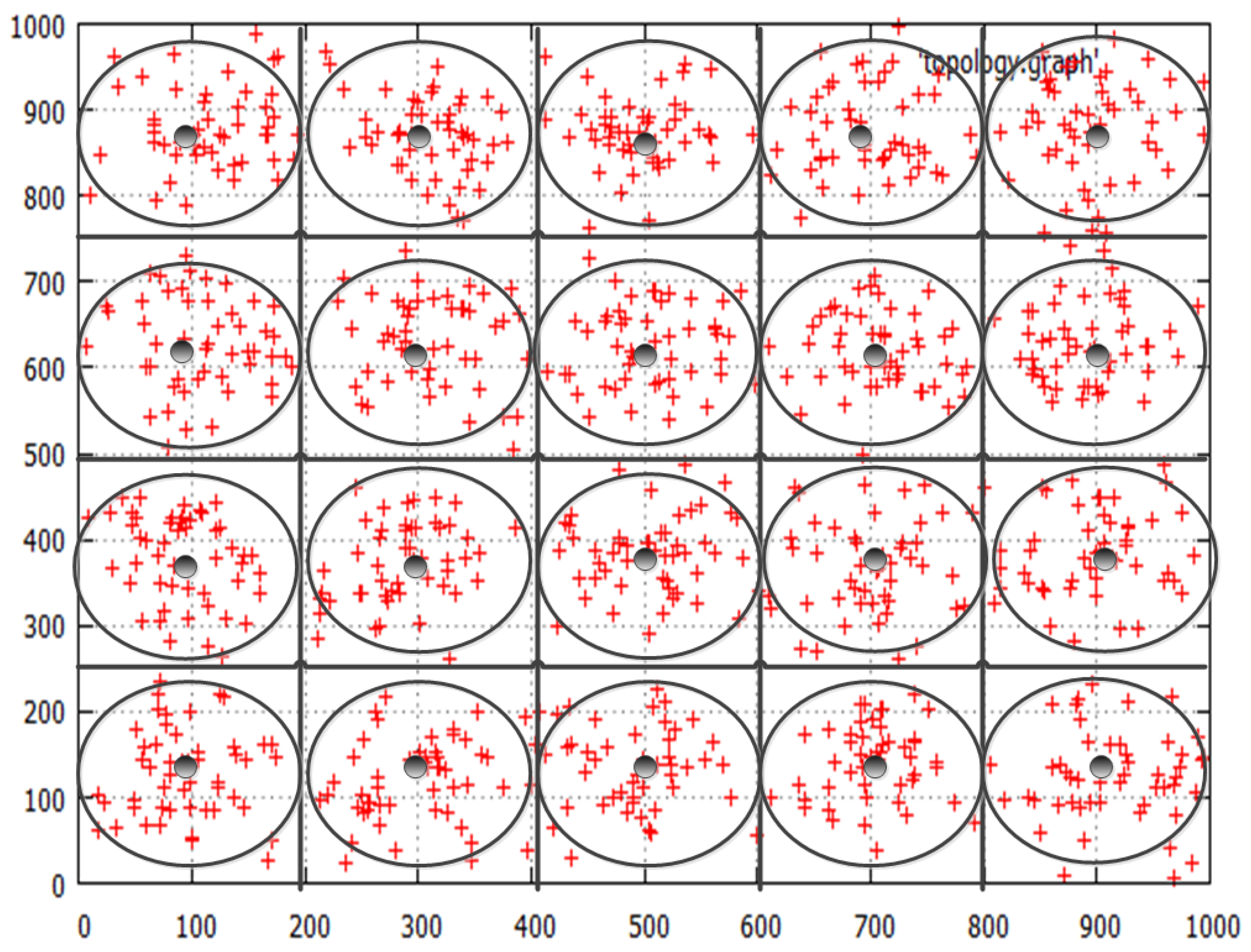
Home Zone
Population Density
Communication
Assumptions
3.2. Adversary Model
- Mobility: The adversary was classified as being either localized or ubiquitous based on his mobility. A localized adversary was limited to injecting replicas within a particular convex sub-area of the sensor field while a ubiquitous adversary had the freedom to traverse the entire network field in his effort to identify, compromise and inject duplicate nodes. In some sense, this captures the degree of physical monitoring or surveillance present in the sensor field. If the sensor network is highly unattended, then perhaps this allows the adversary to freely traverse the entire field without fear of detection. It is of course in the adversary’s best interest to operate in a stealthy manner and attempt to avoid detection, since detection could trigger automated protocols, such as SWATT [34], to sweep the network and remove compromised nodes.
- Intelligence: The adversary was classified as being either oblivious or smart based on his or her intelligence to identify potential target nodes to compromise. The smart adversary chooses to compromise sensor nodes that yield the most benefit, i.e., that maximizes the chances of his or her injected replicas to go undetected, while the oblivious adversary merely compromises a random sensor node oblivious of the processes used in the detection algorithm.
4. Epidemic Diffusion
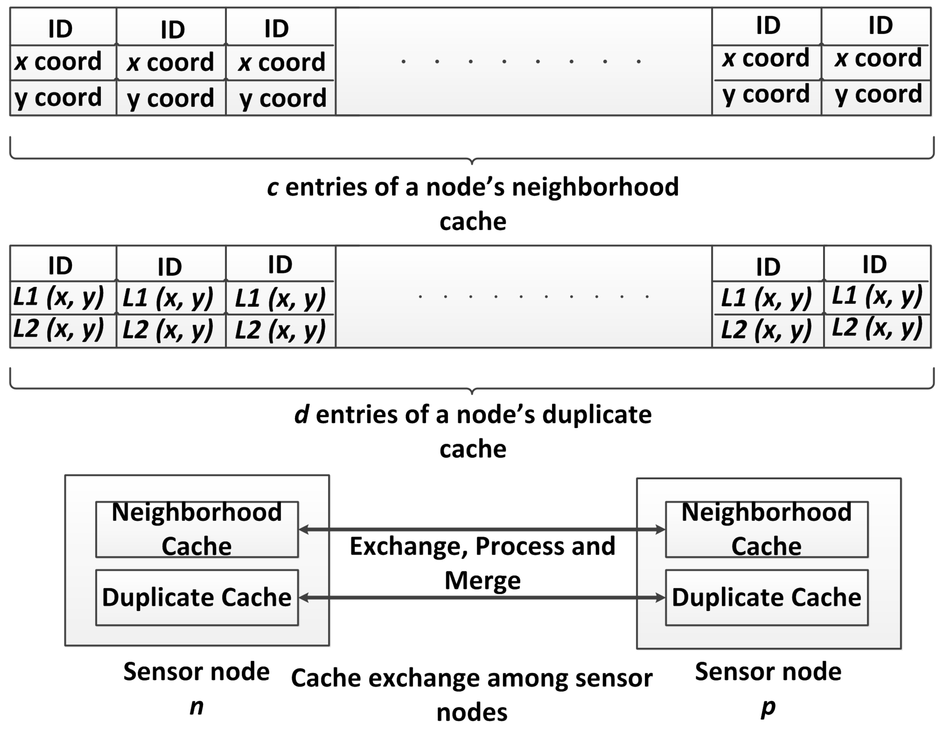
- Primary epidemic: Sensor nodes should detect a duplicate node in their midst by exchanging neighborhood information with each other.
- Secondary epidemic: Once a duplicate node has been detected by a sensor node, this information should be disseminated to the rest of the nodes in the network as soon as possible.
- Direct mail: Each sensor node, upon receiving an infection, immediately transmits this infection to all the other nodes in the network. This method is of course very timely. However, it is quite expensive in terms of communication and node storage. Even assuming that every sensor node possesses complete knowledge of every other node in the network, there are issues of message loss and the bottleneck proportional to the size of the network created at each sending node. Instead of direct mail, one could perhaps use a broadcast mailing mechanism to alleviate these issues. However, such broadcast mailing schemes would necessarily have to rely upon and take advantage of the knowledge of the distributed sensor network and would probably be designed using one of the epidemic primitives discussed below. In fact, such broadcast schemes have been used extensively in earlier duplicate detection in sensor network research, as discussed in Section 2. This is, in spirit, essentially a folklore broadcast distribution mechanism implicit in previous work. However, these prior research works do not explicitly describe the broadcast mechanism used, nor do they precisely analyze the cost incurred by their broadcast schemes, in terms of computation, communication and storage. The costs associated with such broadcasting are typically dismissed by prior researchers as negligible, so long as these broadcast messages are contained within a reasonably small geographic region. In this paper, we account for every interaction between nodes and measure the communication, computation and storage costs precisely.
- Anti-entropy: Each sensor node n periodically contacts another node p at random, and they exchange infections with each other. This exchange can be accomplished in a couple of ways: push, infections known to n, but not to p are sent from n to p; pull, infections known to p, but not to n are sent from p to n; or push-pull, bidirectional information/infection transfer. It has been shown that either pull or push-pull is greatly preferable to push [35] in terms of dissemination speed, and hence, we opted to use the push-pull mechanism in for diffusing the primary and secondary epidemics and describe it in more detail below.
- Rumor mongering: Each sensor node is initially susceptible (has no infection to share). When a node gets infected, this infection, called a rumor, is periodically transmitted (pushed) to a random sensor node in the network. When the node has tried to push its rumor a certain number of times, the node stops transmitting its rumor and is effectively removed in the sense that it becomes inactive. There are a couple of variants proposed by Demers et al. [35], which determine when a node is removed:
- Feedback vs. blind: A sender node is removed with some probability only if it has pushed its rumor to a recipient that already knows the rumor. In blind mode, the sender is removed with some probability regardless of whether the recipient is aware of the rumor and is perhaps better suited in a sensor network scenario, as we could reap some energy/communication savings by eliminating the feedback message from the recipient. Nevertheless, we do not use this scheme and explain our reasoning below.
- Coin vs. counter: In the coin mode, the sender node is removed with some probability based on the flip of its coin. In the counter mode, the sender node is removed with probability one after a certain number of rumor pushing attempts.
- Typically, the feedback/blind and coin/counter modes are combined to obtain schemes, such as coin-blind and feedback-counter modes of operation, for the rumor mongering diffusion scheme.
5. Our Epidemic Algorithm
5.1. Overview
5.2. Discard Duplicate Detection Scheme
| Algorithm 1: duplicate detection protocol: active thread. |
| Data: Protocol run by sensor nodes n and p. Result: Caches updated and duplicates detected.  |
| Algorithm 2: duplicate detection protocol: passive thread. |
| Data: Protocol run by sensor nodes n and p. Result: Caches updated, duplicates detected.  |
6. Security Analysis and Results
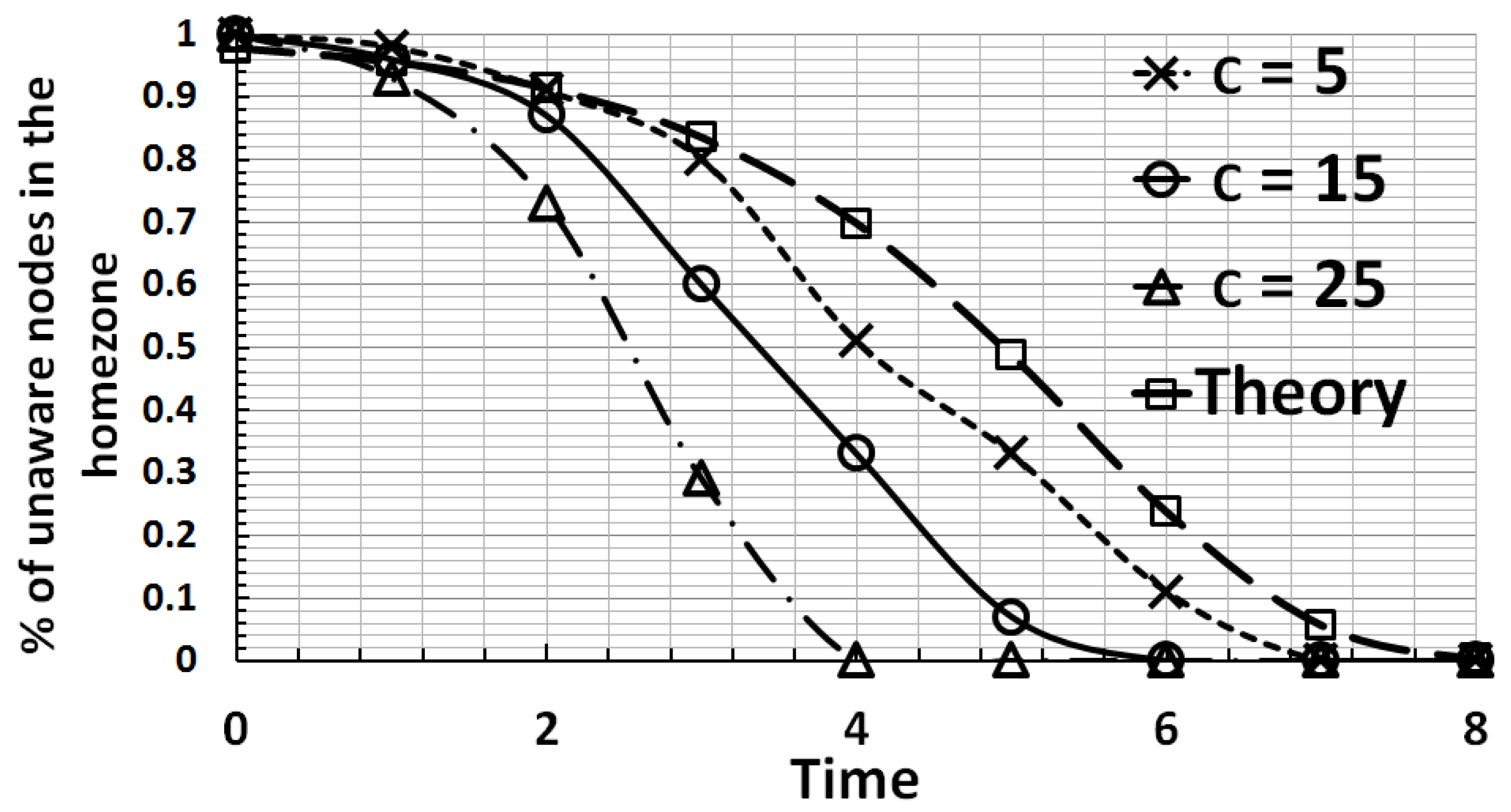
6.1. Detection Time and Accuracy
- If n was not infected at time i,
- The peer sensor node p that n contacted at time i was not infected and
- No peer nodes that were infected contacted n at time i.
6.2. Communication Cost

6.3. Computation Cost
6.4. Storage Cost
6.5. Additional Security Discussions
6.5.1. Need for the Secondary Epidemic
6.5.2. Need for Multiple Verifiers
6.5.3. More than d Duplicates
6.5.4. Revocation
6.5.5. Putting It All Together
6.6. Summary of Our Results and Comparison to Prior Schemes

| Schemes | Communication | Storage | Computation |
|---|---|---|---|
| Broadcast [10] | O() | O(d) | ND |
| RM [10] | O() | O() | ND |
| LSM [10] | O() | O() | ND |
| SET [17] | O() | O(n) | O(1) |
| RED [14,15] | O() | O() | O() |
| SDC [16] | O() | O(1) | ND |
| P-MPC [16] | O() | O(1) | ND |
| Scheme III [18] | O(n) | O(s) | O(1) |
| CSI [45] | O() | ND | ND |
| O(n) | O(1) | O(1) |
- Scheme III by Ho et al. [18] and similar duplicate detecting schemes do not seem to place an emphasis on detecting duplicates within a small geographic region (say, within a home zone). The reasoning is that the adversary can exert his or her influence only within this small region, which is reasonable. However, in our scheme, we detect these duplicates, as well.
- We present an explicit relationship between storage costs and detection accuracy.
- It is also noteworthy that, in , the detection rate is independent of the deployment accuracy. However, as expected, the communication cost of course depends on the deployment accuracy.
- As noted earlier, since every location claim is digitally signed, the adversary cannot make uncompromised nodes appear to be replicas by faking their location claims. Thus, works without any false positives.
- The schemes we outlined in prior work, Section 2, use broadcast mechanisms to propagate duplicate node information in the home zone. However, these broadcast communication costs are typically not accounted for and are deemed negligible. In our scheme, we account for all costs explicitly.
- Lastly, unlike Scheme III by Ho et al. [18], our storage costs are independent of the group size.
- In this paragraph, we sketch a quick comparison of our work with the scheme called CSI [45], depicted in the table above. In the protocol CSI, presented by Yu et al. [45], the detection of duplicate nodes in the sensor network is accomplished by the scheme CSI that employs a novel signal processing technique called compressed sensing. CSI has a communication cost of O(), which the authors show to be the lowest possible communication cost in an unstructured sensor network. However, in our work, we are dealing with a group-deployed static sensor network. To this end, we are able to enjoy a lower communication cost of O(n). Naturally, these two schemes are not directly comparable because of the differences in their underlying network topologies. Furthermore, while the authors demonstrate that CSI has low communication costs, the discussion of computation and storage costs incurred by the scheme for each time period is missing and has not been discussed in the work. Since CSI uses “TAG: a Tiny AGgregationService for Ad-Hoc Sensor Networks” [46] and builds an aggregation tree rooted at the base station among the sensor nodes to accomplish its duplicate detection mechanism, we argue that the storage and computation costs are proportional to the tree generation and maintenance subroutines. This also imposes the requirement that the sensor nodes have been scheduled such that the data can be aggregated along the tree “level-by-level” at each time instant. In summary, while CSI does accomplish duplicate detection efficiently, it does so with the help of underlying subroutines (whose costs are not accounted for) and with a special purpose tree topology, which may or may not be conducive in all deployment models. The same is true of our scheme, as well. also employs a group-deployed structure, and one might argue that this deployment model is not suitable in all circumstances.
7. Implementation Details
8. Future Work and Discussion
9. Conclusions
Acknowledgments
Author Contributions
Conflicts of Interest
References
- Chan, H.; Perrig, A.; Song, D. Random key predistribution schemes for sensor networks. In Proceedings of the 2003 IEEE Symposium on Security and Privacy, Oakland, CA, USA, 11–14 May 2003; pp. 197–213.
- Eschenauer, L.; Gligor, V.D. A key-management scheme for distributed sensor networks. In Proceedings of the 9th ACM Conference on Computer and Communications Security, Washington, DC, USA, 18–22 November 2002; pp. 41–47.
- Akyildiz, I.F.; Su, W.; Sankarasubramaniam, Y.; Cayirci, E. A survey on sensor networks. IEEE Commun. Mag. 2002, 40, 102–114. [Google Scholar] [CrossRef]
- Akyildiz, I.F.; Su, W.; Sankarasubramaniam, Y.; Cayirci, E. Wireless sensor networks: A survey. Comput. Netw. 2002, 38, 393–422. [Google Scholar] [CrossRef]
- Newsome, J.; Shi, E.; Song, D.; Perrig, A. The Sybil attack in sensor networks: Analysis & defenses. In Proceedings of the 3rd International Symposium on Information Processing in Sensor Networks, Berkeley, CA, USA, 26–27 April 2004; pp. 259–268.
- Douceur, J.R. The Sybil attack. In Peer-to-Peer Systems; Springer: Heidelberg, Germany, 2002; pp. 251–260. [Google Scholar]
- Conti, M.; di Pietro, R.; Mancini, L.V.; Mei, A. Emergent properties: Detection of the node-capture attack in mobile wireless sensor networks. In Proceedings of the First ACM Conference on Wireless Network Security, Alexandria, VA, USA, 31 March–2 April 2008; pp. 214–219.
- Shashidhar, N.; Kari, C.; Verma, R. Epidemic Node Replica Detection in Sensor Networks. In Proceedings of the Third IEEE ASE International Conference on Cyber Security (CyberSecurity 2014), Stanford, CA, USA, 27–31 May 2014.
- Brooks, R.; Govindaraju, P.; Pirretti, M.; Vijaykrishnan, N.; Kandemir, M.T. On the detection of clones in sensor networks using random key predistribution. IEEE Trans. Syst. Man Cybern. Part C Appl. Rev. 2007, 37, 1246–1258. [Google Scholar] [CrossRef]
- Parno, B.; Perrig, A.; Gligor, V. Distributed detection of node replication attacks in sensor networks. In Proceedings of the 2005 IEEE Symposium on Security and Privacy, Oakland, CA, USA, 8–11 May 2005; pp. 49–63.
- Xing, K.; Liu, F.; Cheng, X.; Du, D.H. Real-time detection of clone attacks in wireless sensor networks. In Proceedings of the The 28th International Conference on IEEE Distributed Computing Systems, ICDCS’08, Beijing, China, 17–20 June 2008; pp. 3–10.
- Zhu, W.T.; Zhou, J.; Deng, R.H.; Bao, F. Detecting node replication attacks in wireless sensor networks: A survey. J. Netw. Comput. Appl. 2012, 35, 1022–1034. [Google Scholar] [CrossRef]
- Gligor, V. Security of emergent properties in ad-hoc networks (transcript of discussion). In Security Protocols; Springer: Heidelberg, Germany, 2006; pp. 256–266. [Google Scholar]
- Conti, M.; di Pietro, R.; Mancini, L.V.; Mei, A. A randomized, efficient, and distributed protocol for the detection of node replication attacks in wireless sensor networks. In Proceedings of the 8th ACM International Symposium on Mobile Ad Hoc Networking and Computing, Montreal, QC, Canada, 9–14 September 2007; pp. 80–89.
- Conti, M.; di Pietro, R.; Mancini, L.V.; Mei, A. Distributed detection of clone attacks in wireless sensor networks. IEEE Trans. Dependable Secur. Comput. 2011, 8, 685–698. [Google Scholar] [CrossRef]
- Zhu, B.; Addada, V.G.K.; Setia, S.; Jajodia, S.; Roy, S. Efficient distributed detection of node replication attacks in sensor networks. In Proceedings of the Twenty-Third Annual Computer Security Applications Conference, ACSAC 2007, Miami Beach, FL, USA, 10–14 December 2007; pp. 257–267.
- Choi, H.; Zhu, S.; la Porta, T.F. SET: Detecting node clones in sensor networks. In Proceedings of the Third International Conference on Security and Privacy in Communications Networks and the Workshops, SecureComm 2007, Nice, France, 17–21 September 2007; pp. 341–350.
- Ho, J.W.; Liu, D.; Wright, M.; Das, S.K. Distributed detection of replica node attacks with group deployment knowledge in wireless sensor networks. Ad Hoc Netw. 2009, 7, 1476–1488. [Google Scholar] [CrossRef]
- Liu, D.; Ning, P.; Du, W. Group-based key predistribution for wireless sensor networks. ACM Trans. Sens. Netw. (TOSN) 2008, 4. [Google Scholar] [CrossRef]
- Du, W.; Wang, R.; Ning, P. An efficient scheme for authenticating public keys in sensor networks. In Proceedings of the 6th ACM International Symposium on Mobile Ad Hoc Networking and Computing, Chicago, IL, USA, 25–28 May 2005; pp. 58–67.
- Du, W.; Fang, L.; Peng, N. Lad: Localization anomaly detection for wireless sensor networks. J. Parallel Distrib. Comput. 2006, 66, 874–886. [Google Scholar] [CrossRef]
- Du, W.; Deng, J.; Han, Y.S.; Chen, S.; Varshney, P.K. A key management scheme for wireless sensor networks using deployment knowledge. In Proceedings of the Twenty-third AnnualJoint Conference of the IEEE Computer and Communications Societies, INFOCOM 2004, Hong Kong, China, 7–11 March 2004; Volume 1.
- Delgosha, F.; Fekri, F. Threshold key-establishment in distributed sensor networks using a multivariate scheme. In Proceedings of the 25th IEEE International Conference on Computer Communications, INFOCOM 2006, Barcelona, Spain, 23–29 April 2006; pp. 1–12.
- Liu, D.; Ning, P. Establishing pairwise keys in distributed sensor networks. In Proceedings of the 10th ACM Conference on Computer and Communications Security, Washington, DC, USA, 27–30 October 2003; pp. 52–61.
- Zhang, W.; Tran, M.; Zhu, S.; Cao, G. A random perturbation-based scheme for pairwise key establishment in sensor networks. In Proceedings of the 8th ACM International Symposium on Mobile Ad Hoc Networking and Computing, Montreal, QC, Canada, 9–14 September 2007; pp. 90–99.
- Leon-Garcia, A. Probability and Random Processes for Electrical Engineering; Addison-Wesley: Reading, UK, 1994; Volume 2. [Google Scholar]
- Albano, M.; Chessa, S.; Nidito, F.; Pelagatti, S. Dealing with nonuniformity in data centric storage for wireless sensor networks. IEEE Trans. Parallel Distrib. Syst. 2011, 22, 1398–1406. [Google Scholar] [CrossRef]
- Gupta, V.; Wurm, M.; Zhu, Y.; Millard, M.; Fung, S.; Gura, N.; Eberle, H.; Shantz, S.C. Sizzle: A standards-based end-to-end security architecture for the embedded internet. Pervasive Mob. Comput. 2005, 1, 425–445. [Google Scholar] [CrossRef]
- Liu, A.; Ning, P. TinyECC: A configurable library for elliptic curve cryptography in wireless sensor networks. In Proceedings of the International Conference on Information Processing in Sensor Networks, IPSN’08, St. Louis, MO, USA, 22–24 April 2008; pp. 245–256.
- Wang, H.; Sheng, B.; Tan, C.C.; Li, Q. Comparing symmetric-key and public-key based security schemes in sensor networks: A case study of user access control. In Proceedings of the 28th International Conference on Distributed Computing Systems, ICDCS’08, Beijing, China, 17–20 June 2008; pp. 11–18.
- Liu, D.; Ning, P.; Du, W.K. Attack-resistant location estimation in sensor networks. In Proceedings of the 4th International Symposium on Information Processing in Sensor Networks, Los Angeles, CA, USA, 25–27 April 2005; p. 13.
- Li, Z.; Trappe, W.; Zhang, Y.; Nath, B. Robust statistical methods for securing wireless localization in sensor networks. In Proceedings of the Fourth International Symposium on Information Processing in Sensor Networks, IPSN 2005, Los Angeles, CA, USA, 25–27 April 2005; pp. 91–98.
- Capkun, S.; Hubaux, J.P. Secure positioning in wireless networks. IEEE J. Sel. Areas Commun. 2006, 24, 221–232. [Google Scholar] [CrossRef]
- Seshadri, A.; Perrig, A.; van Doorn, L.; Khosla, P. Swatt: Software-based attestation for embedded devices. In Proceedings of the 2004 IEEE Symposium on Security and Privacy, Oakland, CA, USA, 9–12 May 2004; pp. 272–282.
- Demers, A.; Greene, D.; Hauser, C.; Irish, W.; Larson, J.; Shenker, S.; Sturgis, H.; Swinehart, D.; Terry, D. Epidemic algorithms for replicated database maintenance. In Proceedings of the Sixth Annual Acm Symposium on Principles of Distributed Computing, Vancouver, BC, Canada, 10–12 August 1987; pp. 1–12.
- Eugster, P.T.; Guerraoui, R.; Kermarrec, A.M.; Massoulié, L. From epidemics to distributed computing. IEEE Comput. 2004, 37, 60–67. [Google Scholar] [CrossRef]
- Bailey, N.T. The Mathematical Theory of Infectious Diseases and Its Applications; Hafner Press/ MacMillian Pub. Co.: New York, NY, USA, 1975. [Google Scholar]
- Albano, M.; Gao, J. In-network coding for resilient sensor data storage and efficient data mule collection. In Algorithms for Sensor Systems; Springer: Heidelberg, Germany, 2010; pp. 105–117. [Google Scholar]
- Xu, Y.; Heidemann, J.; Estrin, D. Geography-informed energy conservation for ad hoc routing. In Proceedings of the 7th Annual International Conference on Mobile Computing and Networking, Rome, Italy, 16–21 July 2001; pp. 70–84.
- Wander, A.S.; Gura, N.; Eberle, H.; Gupta, V.; Shantz, S.C. Energy analysis of public-key cryptography for wireless sensor networks. In Proceedings of the Third IEEE International Conference on Pervasive Computing and Communications, PerCom 2005, Kauai Island, HI, USA, 8–12 March 2005; pp. 324–328.
- Eugster, P.T.; Guerraoui, R.; Handurukande, S.B.; Kouznetsov, P.; Kermarrec, A.M. Lightweight probabilistic broadcast. ACM Trans. Comput. Syst. (TOCS) 2003, 21, 341–374. [Google Scholar] [CrossRef]
- Jelasity, M.; Kowalczyk, W.; van Steen, M. Newscast Computing; Technical Report IR-CS-006; Vrije Universiteit Amsterdam, Department of Computer Science: Amsterdam, The Netherlands, 2003. [Google Scholar]
- DataSheet, M. Crossbow Technology; Document Part Number: 6020-0042-08 Rev A; 2013. [Google Scholar]
- Barot, M.; de la Peña, J.A. Estimating the size of a union of random subsets of fixed cardinality. Elem. Math. 2001, 56, 163–169. [Google Scholar] [CrossRef]
- Yu, C.M.; Lu, C.S.; Kuo, S.Y. CSI: Compressed sensing-based clone identification in sensor networks. In Proceedings of the 2012 IEEE International Conference on Pervasive Computing and Communications Workshops (PERCOM Workshops), Lugano, Switzerland, 19–23 March 2012; pp. 290–295.
- Madden, S.; Franklin, M.J.; Hellerstein, J.M.; Hong, W. TAG: A tiny aggregation service for ad-hoc sensor networks. ACM SIGOPS Oper. Syst. Rev. 2002, 36, 131–146. [Google Scholar] [CrossRef]
- Montresor, A.; Jelasity, M. PeerSim: A Scalable P2P Simulator. In Proceedings of the 9th International Conference on Peer-to-Peer (P2P’09), Seattle, WA, USA, 9–11 September 2009; pp. 99–100.
- Richa, A.W.; Mitzenmacher, M.; Sitaraman, R. The power of two random choices: A survey of techniques and results. Comb. Optim. 2001, 9, 255–304. [Google Scholar]
© 2015 by the authors; licensee MDPI, Basel, Switzerland. This article is an open access article distributed under the terms and conditions of the Creative Commons Attribution license (http://creativecommons.org/licenses/by/4.0/).
Share and Cite
Shashidhar, N.; Kari, C.; Verma, R. The Efficacy of Epidemic Algorithms on Detecting Node Replicas in Wireless Sensor Networks. J. Sens. Actuator Netw. 2015, 4, 378-409. https://doi.org/10.3390/jsan4040378
Shashidhar N, Kari C, Verma R. The Efficacy of Epidemic Algorithms on Detecting Node Replicas in Wireless Sensor Networks. Journal of Sensor and Actuator Networks. 2015; 4(4):378-409. https://doi.org/10.3390/jsan4040378
Chicago/Turabian StyleShashidhar, Narasimha, Chadi Kari, and Rakesh Verma. 2015. "The Efficacy of Epidemic Algorithms on Detecting Node Replicas in Wireless Sensor Networks" Journal of Sensor and Actuator Networks 4, no. 4: 378-409. https://doi.org/10.3390/jsan4040378