1. Introduction
Network coding was originally proposed in wired networks and for multicast transmissions only [
1,
2]. Soon, it was discovered that the broadcast nature of wireless transmissions was amenable to network coding, and inter-flow network coding was then proposed to exploit this technique for unicast scenarios [
3]. Nodes in the wireless network may overhear packets that are not meant for them. Instead of discarding these packets, nodes can choose to store them temporarily and use them later to decode coded packets, therefore reducing the total required number of transmissions to fulfil certain transmission tasks. The XOR-based coding scheme is the simplest yet effective coding scheme applied. Two or more packets can be XOR-ed together, and a destination node can extract the original packet from the coded packet by looking in its overheard packet buffer.
Existing protocols that utilize the power of network coding usually take the most straightforward means to do network-packet scheduling, namely round-robin scheduling. Basically, an intermediate node will construct many queues, each storing packets from a specific flow/session. When the MAC layer obtains the right to transmit, the network layer selects the packet to be sent in a round-robin fashion across all queues. When a certain queue is selected, the first packet in that queue is dequeued, and it goes through a check for coding opportunity. Coding opportunities are depicted in a coding graph [
4]. In this graph, each vertex denotes a flow that passes by. An edge that links two vertices means that packets from the respective flows can be coded together. When three flows can be coded together, it is shown as a triangle. Similarly,
N coding-possible flows are denoted as a complete
N-vertex sub-graph, a.k.a.
N-clique.
However, with this scheduling, we do not have much control over the performance of the network (namely, per-flow throughput and fairness). Some flows may be repeatedly transmitted, because they can be coded with many other flows, while some flows with less or no coding counterparts can starve. In addition, it is possible that we can increase the throughput by intelligently selecting the set of packets to transmit.
In this work, we first study a simplified and static form of the scheduling problem. When given a set of packets from multiple flows in a queue, we analyze how to empty the queue with the minimum number of transmissions. This problem is abstracted and formulated as a weighted clique cover problem (WCCP). WCCP is NP-hard as a whole, and some special cases of it can be solved in polynomial time. In order to account for the general case, a search algorithm with pruning and approximation is proposed. With this algorithm, the solution can be calculated much faster with known error bounds.
The solution to this static problem can then provide guidance to find the solution to the real problem, i.e., the dynamic form of the problem. In this form, we consider that a node is an intermediate node for multiple flows. A number of fixed-length queues are embedded in this node with packets stochastically arriving. The processing speed is also limited. We estimate the fairness with two relevant performance metrics: one is the minimum throughput and the other is the variance of the throughputs of all flows. A higher minimum throughput and smaller throughput variance imply better fairness. Our objective is to find an optimal scheduling scheme, which first maximizes fairness, then maximizes throughput. We use a heuristic scheduling method for this dynamic form of the problem.
The contributions of this paper are mainly two-fold:
- (1)
We raised concerns about the coding-aware packet scheduling method. This usually-neglected field of research can actually lead to significant performance improvement in coding-enabled networks. In addition, further analysis into the scheduling method opens up many more possibilities. One can easily plug in a different performance metric other than the one we adopted and arrive at a totally different scheduling method that achieves a new balance between fairness and throughput gain.
- (2)
Technically, we provided a step-by-step decomposition of the complex coding-aware scheduling problem. Even though the problem is mathematically hard to tackle (for its being NP-complete), we managed to produce decent solutions within tractable cost. The results and experiences we gained can be beneficial to other researchers.
In
Section 2, we review the existing coding-aware scheduling algorithms.
Section 3 formulates the static scheduling problem as a WCCP and proposes an approximation algorithm.
Section 4 describes the dynamic form of the problem, and we propose here a heuristic scheduling scheme.
Section 3 and
Section 4 contain some preliminary evaluations.
Section 5 presents the scheduling scheme in the form of a routing protocol, and a series of network simulations is done to evaluate the performance of this protocol. Lastly, we conclude in
Section 6.
2. Related Works
In this section, we refer readers to a few related works that considered the scheduling problem with network coding. Additional literature on the problem formulation and solution are described along the main body of the paper.
Network coding is a great fit for wireless networks. Fragouli
et al. [
5] study the case of applying network coding in wireless networks in many aspects. These include throughput, reliability, mobility and management. Several key challenges are proposed, as well.
There are many researchers working on the topic of scheduling in network coding settings. However, most of them focus only on MAC-layer scheduling. The method usually gives “higher priority” to coding nodes. Sagduyu
et al. [
6,
7,
8,
9] give examples of this kind.
In addition to MAC-layer scheduling, there are other novel solutions that involve scheduling. Yomo and Popovski [
10] propose an opportunistic scheduling algorithm. The links between the intermediate nodes and receiver nodes are subject to channel fading. When this fading is time-varying, the authors propose an opportunistic network coding scheme to determine how many and which packets are coded. It is shown that such an opportunistic scheme can provide higher throughput than any coding scheme that involves a fixed number of packets. Ni
et al. [
11] discuss the optimal physical-layer transmission rate in the MIT
Roofnetplatform. The basic idea is that a lower rate gives rise to a longer transmission range or a higher delivery ratio. Furthermore, the distances from the intermediate node to the two recipients may not be the same. Therefore, their delivery ratios would be different. In 802.11b, if 5.5 Mbps or 11 Mbps is used, the total expected coded transmission time (ECT) can be different.
Most network-coding schemes are agnostic about the PHYand MAC layer. They assume a greedy algorithm to enforce network coding. However, Chaporkar and Proutiere [
12] advocate that exploiting every opportunity to enforce network coding may downgrade the overall throughput of the system. The statement is demonstrated using a scenario where interference is incorporated into the analysis. Hence, a specially tailored MAC-layer scheduling algorithm is proposed in order to achieve the expected throughput gain.
Zhao and Yang [
13] consider the joint scheduling problem for MIMO and network coding (MIMO-NC) in wireless networks. A network in which each node is equipped with two antennas is analyzed. In order to achieve higher throughput, the authors propose a packet scheduling algorithm, which in essence matches all source-destination flows into pairs. When a pair is discovered, MIMO-NC is applied to reduce the number of transmissions. However, this approach requires the full knowledge of the network and traffic patterns. In addition, it is highly dependent on the traffic pattern. When the prescribed pair is not available, the power of MIMO is then wasted.
3. The Static Form of the Problem
We formally define the “problem” under consideration here. That is, we aim to devise a total solution in the network layer to answer the question: How does one coordinate the routing and packet scheduling in a wireless network, so that the overall performance of the network is optimized? By “performance”, we jointly consider the fairness and end-to-end throughput among flows.
The methodology we took was to find the optimal solution to a simplified version of the problem and then gradually add complexity into the problem, enriching the solution on the fly. The mostly abstracted version of the scheduling problem is its static form, which is in our work abstracted as a weighted clique cover problem.
3.1. Weighted Clique Cover Problem
Consider an isolated scenario with only one node. This node has multiple queues of packets. Packets from some of the queues can be coded together, while others cannot. This relationship is depicted in a coding graph, where each vertex represents one queue and each edge represents a coding-possible relationship between two queues. A set of k packets can be coded and sent in one transmission if and only if they come from k distinct queues (k vertices) and each pair of queues is coding-possible ( edges). The objective is to find a scheduling algorithm that minimizes the number of transmissions, either coded or non-coded, to empty all queues. This problem is called static in the sense that no new packets would arrive.
This problem is mathematically formulated as a weighted clique cover problem as below:
Definition 1 (Weighted clique cover problem).
Given a graph ,
where V is the set of vertices, E is the set of edges and a weight function that maps each vertex to a positive integer, we define a weighted clique w.r.t. the graph as ,
where is a set of vertices that are fully connected in G (
i.e.,
is the vertex set of a clique in G) and is a positive integer that satisfies: We then further define a weighted clique cover w.r.t. the weighted graph as a set of weighted cliques ,
such that: The problem is to find a weighted clique cover w.r.t. the weighted graph that minimizes .
As one of the 21 Karp’s NP-complete problems [
14], the clique cover problem (CCP) is NP-complete. WCCP, as a generalized form of CCP, is known to be NP-complete, as well, and researchers have been working on a practical solution to it. It is shown by Hsu [
15,
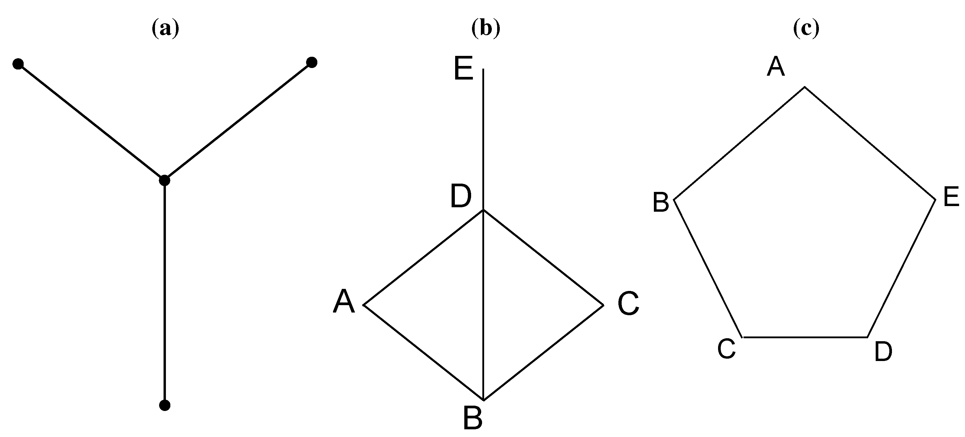
16] that for a special class of graphs, known as claw-free perfect graphs, the WCCP problem can be solved in polynomial time. A claw is the shape shown in
Figure 1a. It is often referred to as
, because it is essentially 1,3-bipartite. A claw-free graph is a graph where none of its sub-graphs is a claw. A perfect graph was an idea raised in the 1970s by Claude Berge [
17]. Mathematically, a graph is said to be perfect if, for each of its induced sub-graphs, the chromatic number equals the size of its largest clique of the subgraph. Take
Figure 1b as an example. Nodes
A,
B,
D,
E can form a sub-graph. The corresponding induced sub-graph contains the four nodes, as well as the four edges that connect them. In this induced sub-graph, the chromatic number is three, because we can color Nodes
A and
E as red, Node
D as green and Node
B as green, such that no adjacent nodes have the same color. The size of the maximum clique in this sub-graph is also three, as Nodes
A,
B and
D form a three-node clique. The simplest imperfect graph is a ring of five nodes shown in
Figure 1c. The size of the maximum clique is two, but the chromatic number is three. A more recent paper [
18] summarizes the problem and some recent advances on the topic.
Figure 1.
There exists polynomial solutions to the weighted clique cover problem (WCCP) for claw-free perfect graphs. (a) Illustration of a claw; (b) an example of a perfect graph; (c) an example of an imperfect graph.
Figure 1.
There exists polynomial solutions to the weighted clique cover problem (WCCP) for claw-free perfect graphs. (a) Illustration of a claw; (b) an example of a perfect graph; (c) an example of an imperfect graph.
3.2. Solution to WCCP
As the size of the problem (i.e., the number of vertices, the number of edges and the amount of weights) scales up, WCCP becomes very hard to tackle. Existing polynomial solutions focus only on claw-free perfect graphs. However, claw-free graphs are rare in practice. For practical problems that we may encounter in networks, we need a definitive method to solve them, irrespective of whether they are claw-free or not.
Here, we propose a search-based algorithm to solve WCCP for all perfect graphs (which is more general than the existing algorithms). This algorithm can run in linear time for most of the cases (when pruning is applicable). Note that pruning can be applied even when the graph has claw sub-graphs and is imperfect. After each iteration of pruning, the graph can be modified, and this usually yields a simpler graph. In some extreme cases, its running time grows exponentially with the size of the graph (when pruning is not applicable); we therefore introduce an approximation method to guarantee that the run time is invariant to the amount of weights. Fortunately, these extreme cases are hardly seen in the settings of wireless communication [
19], and they are very difficult to construct, even in the pure mathematical setting.
In essence, our algorithm is a search algorithm that structures all possible solutions into a tree structure. Consider the WCCP in such a way: for each vertex in the graph, its weight equals the sum of the weights of all cliques of which this vertex is a part. Then, if we can list all cliques that one vertex is a part of, the search of cliques that cover the graph can be transformed into the search for a method to allocate weights to a node’s participating cliques, as will soon be defined in Definition 2. The transformation of “covering” to “allocation” enables an iteration-based approach. We iteratively allocate a weight for each vertex. When all vertices have their weights allocated, the solution to WCCP is determined. The search tree is equivalent to a decision tree.
The root node of the search tree denotes the initial state of the problem. As we go down one level, a decision is made at each vertex. After
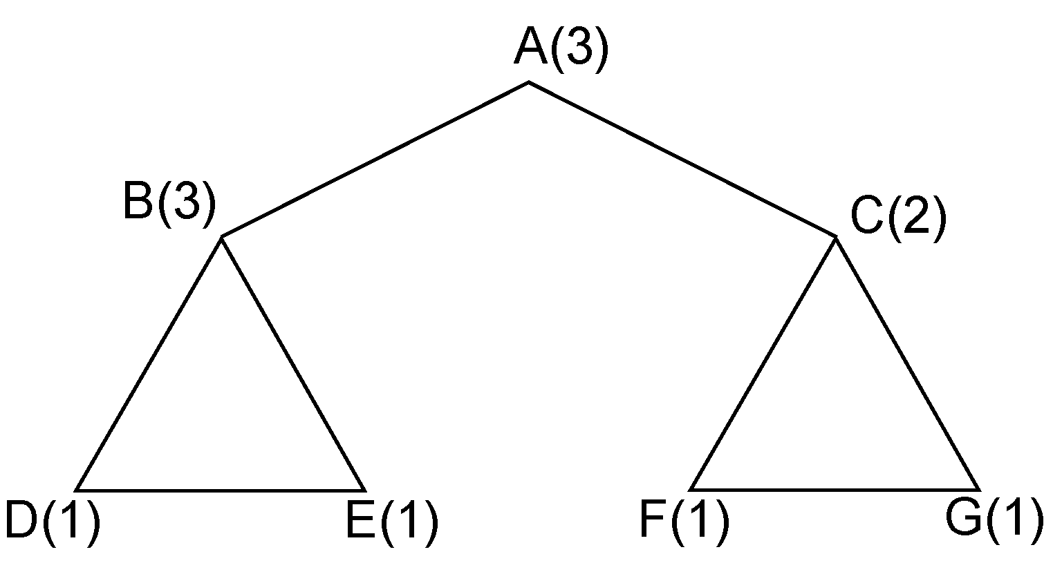
levels, with the respective decision made at every vertex, one solution, or a weighted clique cover, is determined at each leaf node. For example, consider the coding graph shown in
Figure 2. The first search decision can be made at the central vertex
A. Its weight (three) should be allocated to three adjacent cliques,
,
and
. However, due to the fact that
, we can omit the last clique and allocate its weight only to the first two cliques. This will be justified with the introduction of pruning rules in
Section 3.2.1. The allocation can be done in three possible ways:
and
between cliques
and
. Therefore, in the first layer, we have three branching nodes, each of which denotes one choice of possible allocations.
Figure 2.
One example of a coding graph.
Figure 2.
One example of a coding graph.
If we continue the search in this manner, it is a brute-force algorithm that has a time complexity of , where and D is the average number of participating cliques that one vertex can be in. In simple graphs, D is close to the average degree of vertices, which is easier to calculate. In real cases, since , , the complexity can be simplified as . This is obviously unacceptable, as the scale factors are both on the base and the exponent. Therefore, we seek a better algorithm through pruning and approximation.
3.2.1. Pruning
Before describing the pruning mechanism, we first formally define a concept—participating cliques.
Definition 2 (Participating clique).
In a graph , a participating clique of a given vertex is any clique , such that .
Before branching on one vertex, we need to get all of its participating cliques; the number of branches then is dependent on the number of ways to allocate weights to these participating cliques. The pruning rule below demonstrates that we only need to consider a subset of these participating cliques in certain cases, and hence, we can significantly reduce the amount of computation. denotes the set of neighbor vertices of vertex v.
Theorem 3 (Pruning rule).
For a vertex , where , a participating clique of vcan be safely ignored when making the branching decision if it is subsumed by another participating clique ,i.e., . Stated another way, allocating zero weight to the clique will not eliminate the possibility of finding the optimal solution in the pruned search tree.
Proof. Suppose in one optimal allocation, vertex v allocates to clique . We use to denote the difference vertices set between clique and . For each , we assert that must allocate at least to some of its participating cliques that do not have vertex v involved. The reason is stated as below: for every unit of weight of , its allocation may either fall in a clique that involves v or fall in a clique that does not involve v. With , can allocate at most to cliques that involve v. Furthermore, with our assumption that v has allocated to , where is not part, can then allocate at most to cliques that involve v. Therefore, must allocate at least to cliques that do not involve v, just as we have asserted. Consider the following reallocation: For each , we withdraw weights from cliques that do not involve v. This withdrawal either shrinks the vertex set for some cliques or it totally eliminates some cliques with only one vertex inside. In fact, the latter case will never happen if the prior allocation is optimal. Then, these withdrawn weights are merged into the weighted clique with weights, yielding a weighted clique with weights. This reallocation will never increase the sum of weights of weighted cliques, so the new allocation is also optimal. From a local view, the decision to allocate zero weight to clique can therefore never go wrong, and the possibility of reaching optimality is preserved after the decision. ☐
In the following, we give several corollaries to further demonstrate the usage of this pruning rule.
Corollary 4 (One-degree vertex).
In WCCP, if there exists a degree-one vertex connecting to another vertex , allocating to the two-vertex clique will not eliminate the possibility of finding optimal solution in this branch.
Proof. The vertex has only one neighbor , so its participating cliques are and . Since the former clique is subsumed by the latter one, we can allocate zero weight to the one-node clique if . For the cases when , we can allocate at most to the clique . Following the same reallocation-based logic in the proof of Theorem 3, we can assert that this decision will not eliminate the possibility of finding the optimal solution either. ☐
Corollary 5 (
m-degree vertex).
In WCCP, if there exists an m-degree () vertex and together with its m neighbors form a -vertex clique , allocating to the clique will not eliminate the possibility of finding the optimal solution in this branch.
The proof of this corollary follows the same logic as the proof of Corollary 4.
3.2.2. Approximation
So far, we have discussed the pruning rule. When the pruning rule is carried out at a node, the number of branches at this node in the search tree is significantly reduced. However, what happens when no pruning rule is applicable? We use quantization to remove the scale effect of the weights on vertices.
We first determine a parameter Q in the algorithm. Q denotes the level of quantization of weights used in the search algorithm. Consider a vertex with W weights and D participating cliques. In the brute-force search algorithm, we will have branches at this node, because there are a total of ways to allocate weights to the participating cliques. In our approximation algorithm, the total number of weights is split into Q equal shares, and these Q shares are allocated to participating cliques instead. Therefore, the number of branches at this node is reduced to .
We then analyze the amount of error introduced in the approximation step. For a single vertex, its weight can be arbitrarily allocated to its participating cliques. However, due to quantization, each participating clique can only be assigned an integer multiple of m as its weight. Suppose that a real optimal allocation exists and is denoted by , and the “optimal” allocation found by our search algorithm is Σ. We derive by comparing the allocated weights for each participating clique. Consider the transformation from to Σ. Any negative value in implies a revocation of weights for the clique in allocation ; any positive value in implies a reallocation to the corresponding clique. Note that any revocation or reallocation involves at most one share of quantized weight, and this is exactly of the number of weights in the original problem. The size of the problem is reduced to of the original problem, and we can derive that the error involved is limited to .
3.3. Scalability and Error Analysis
3.3.1. Scalability
We use Gilbert’s random graph model [
20] to randomly generate test coding graphs. This model generates graphs by
, where
N denotes the number of vertices and
p denotes the probability by which each edge is selected. For each set of parameters, we generate 25 random graphs and test our algorithm, as well as a non-approximation algorithm (NA). Though the number 25 is chosen arbitrarily, it turns out to be sufficient to demonstrate the performance differences. The non-approximation algorithm also has the feature of pruning unnecessary branches, but it does not quantize total weights into blocks. Therefore, it needs to consider a lot more branches when no pruning rule is applicable, but the solution it provides is an accurate answer.
Since WCCP solves the problem on a weighted graph, weight information should be attached to the randomly generated graphs. In this evaluation, we set the weights assigned to each vertex to be a random variable conforming to a log-normal distribution. Log-normal distribution is chosen, because it is the simplest yet practical distribution for real-life variables with positive values, finite mean and finite variance. By adjusting the mean and standard deviation of this log-normal distribution, we are able to test the algorithm with different scales of weights. The
Colt (
http://acs.lbl.gov/ACSSoftware/colt/) library is the back-end for the random number generator.
The setting of the simulation environment is as follows: Intel i5-3570 3.40 GHz, 8 GB memory, Windows 7 Enterprise 64-bit SP1. Because some of the test graphs are so complicated that it is impractical to wait so long for the result, we take a different approach to measure the run time when the program has been running for too long. We keep track of the amount of search tasks in the program. When the program has run for 10 min and is still running, we estimate the total run time by dividing 10 min by the proportion that has finished searching. We have tested the validity of this approach for some of the scenarios when the estimation is above 10 min but below two hours; the estimation error is generally within 20%. Since we are more concerned about the order of magnitude instead of the absolute value, this error is acceptable. In addition, even though the 25 graphs are generated using the same set of parameters, their processing times can span from milliseconds to days or more. In order to capture this distribution, we take the median value among these 25 values and draw the figures.
The baseline scenario is set with the parameters shown in
Table 1. This baseline is chosen after weighing two factors. Firstly, we want the scenario to be of some complexity. However, secondly, we want to keep the size of the maximum clique as smaller than six. This number is worked out in [
19] as the theoretical maximum clique size in a coding graph. By setting the probability of generating a six-node clique as 5%, we have worked out the baseline parameters. Then, we evaluate the performance of the algorithm by adjusting each single parameter. Note that the ratio between the mean and the standard deviation is fixed at 2:1 for the log-normal distribution.
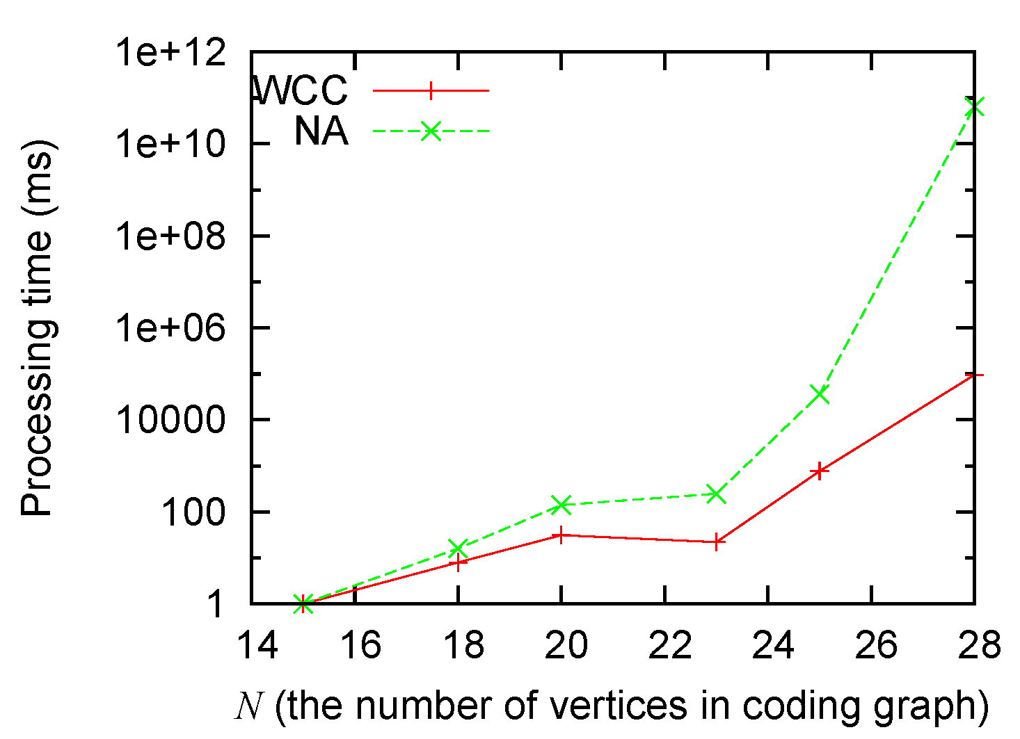
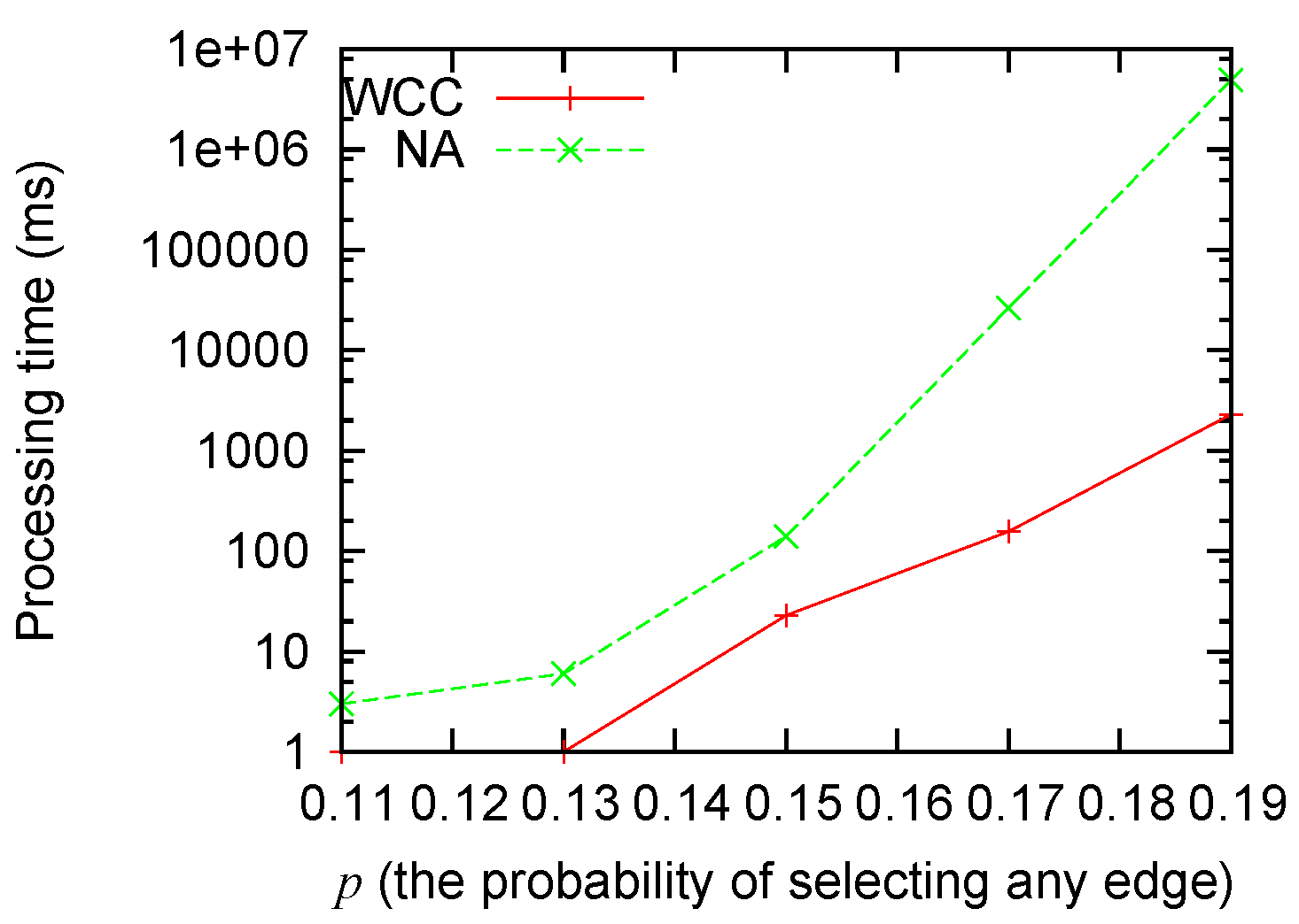
Figure 3 and
Figure 4 show that: (1) the processing time grows for both algorithms when the size of the problem grows; (2) our algorithm consistently runs faster than the non-approximation algorithm; and (3) the improvement (as big as several orders of magnitude) is most significant when the scale of the problem is big.
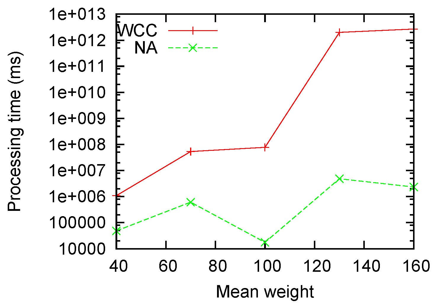
Figure 5 measures the performance with different mean weights. It is clear that our algorithm is roughly invariant on the weight factor, while the non-approximation algorithm grows exponentially with the mean weights.
Table 1.
Baseline scenario parameter settings.
Table 1.
Baseline scenario parameter settings.
| Parameter | N | p | Mean | | Q |
|---|
| Value | 20 | 0.15 | 100 | 50 | 10 |
Figure 3.
Processing time sensitivity to N.
Figure 3.
Processing time sensitivity to N.
Figure 4.
Processing time sensitivity to p.
Figure 4.
Processing time sensitivity to p.
Figure 5.
Processing time sensitivity to .
Figure 5.
Processing time sensitivity to .
3.3.2. Error Analysis
Even though we have derived an upper bound for the approximation error introduced, we are still interested in typical values. In fact, we observe in most cases that the error level is significantly lower than the upper bound. Given a set of parameters, we define the error rate as the probability of getting a scenario that results in an error out of all of the generated scenarios. The average error is defined as the average amount of error over all of the cases. Since the program stops at the 10th minute, any scenario with a running time longer than 10 min does not come with a precise result value. Therefore, we only sample the ones that have results worked out within 10 min.
Surprisingly, the measured error is significantly lower than what we have expected. Within the three sets of experiments where we adjust N, p and , the error rate are 1.92%, 1.08% and 6.38%, respectively. The average errors are also very small, at 0.17%, 0.09% and 0.15%, respectively. Therefore, the overall error rate is much smaller than the upper bound we set, which is 5%. Note that the overall error rate is given by the error rate multiplied by the average error, as we have defined. Further analysis leads us to conclude that this is because of the limit we put on the processing time. For those test cases where the processing time is longer than 10 min, there is a higher probability of getting an error because of the greater amount of branching. Now that we have excluded those cases, the measured error level is underestimated. Nevertheless, this experiment at least gives us some hints on the level of error introduced. It also demonstrates that in real-life scenarios with real-time processing requirements, the error introduced is negligible.
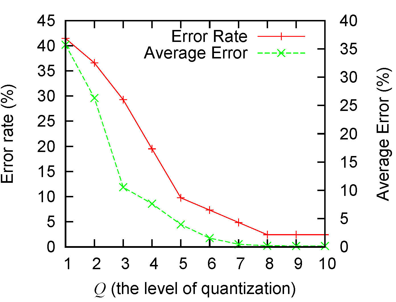
We also measure the amount of error introduced by adjusting the parameter
Q. A larger
Q means a finer quantization and usually less error, as analyzed in
Section 3.2.2. A smaller
Q will lead to higher levels of errors. The extreme case of
is in essence a naive “all-or-none” algorithm. From
Figure 6 we observe that: (1) our algorithm performs significantly better than the naive solution; and (2) a
Q value greater than five can give good-enough performance (with empirical errors smaller than 5%). The values in
Figure 6 are obtained by running the baseline scenario 50 times. Both the error rate and the average error are presented in the figure.
Figure 6.
The error rate and average error with different Q values.
Figure 6.
The error rate and average error with different Q values.
4. The Dynamic Form of the Problem
So far, we have analyzed the scheduling problem, where no new packets would arrive, a.k.a. the static form. In this section, we will relax this restriction and study the problem when new packets are arriving, while queued packets are being processed. The transmission capacity is also considered, as it can be a restricting condition. These factors introduce dynamics into the problem, so it is termed the dynamic form.
Before designing the scheduling method, we need to define the optimization target. When taking into account transmission capacity, we need to consider the trade-off between throughput and fairness. Note that existing coding-aware scheduling methods (e.g., round-robin) have no control over this trade-off at all. In order to avoid unnecessary complexity in describing the scheduling scheme, we discuss only two extreme cases. The first is putting maximal throughput at the highest priority. Among all possible ways to maximize throughput, we choose the one that achieves the best fairness. The second case is the other way around, putting fairness over throughput. In fact, the second case is more sophisticated and its solution reflects all of the tools that we use in designing the scheme for the first case. Therefore, only the second case is expanded in the following.
A naive solution to the dynamic problem would be to blindly apply the solution from the static problem with slight modification. Consider that the algorithm for the static problem can be applied successively to the dynamic form of the scheduling problem periodically. We only need to substitute the number of packets in the packet queues with the expected number of packets that would arrive per second. The scheduling decisions obtained this way can then be used to schedule packets dynamically.
However, this approach is subject to several problems. The adverse effect of dynamic packet arrivals is two-fold:
- (1)
Some flows may have no queued packets when the node is ready to transmit. This waste of bandwidth would decrease the throughput.
- (2)
Some flows may have packets coming faster than they are being processed, resulting in queue overflows. The static solution has never considered the transmitting capacity of nodes and, thus, cannot guarantee better performance when the network is saturated.
Dynamic packet arrivals may introduce opportunities, as well. In the static setting, very often, some “leftover” packets cannot be coded or fully coded, because there are no other packets left with which to be coded. This situation is very much alleviated in the dynamic case, as this shortage of packets will recover sooner or later.
There is another important change resulting from random packet arrivals. The dynamic form of the problem has no deterministic optimal solutions. Moreover, due to the fact that packet arrivals are usually bursty and error-prone, it is even impossible to work out an “optimal” solution in the probabilistic measure. However, fortunately, this lack of “optimal” solution does not mean that we can do nothing to improve the round-robin scheduling. In the following, we take a heuristic approach to optimize the scheduling decision.
4.1. Heuristic Scheduling
The objective of dynamic scheduling is to get higher throughput given the capacity of the network and to maintain a relative fairness among all flows when the network is saturated.
The starting point of this scheduling method is the naive solution that we mention above. First, we translate the offered loads of flows into the expected number of packets that would arrive in one second. These figures are used as the weight in WCCP, and from here, a static solution is obtained in the form of a set of weighted cliques. We will refer to this solution as the initial plan.
The first heuristic rule is to overcome the restriction of transmission capacity. The capacity of a node can be estimated by monitoring the transmission history. When the capacity is smaller than the arrival rate, flows with heavy traffic should be cut off, while flows with less traffic remain intact. Basically, we use the generate-quota algorithm shown in Algorithm 1 to allocate the limited transmission capacity. The final set of weights for all cliques obtained in this step is called a quota, and it is the starting point for further steps. The idea is to maximize the minimum share of quota, while utilizing the coding benefits. If the flow with the smallest offered load can be fully processed, we first allocate the quota accordingly to cover this smallest offered load for all flows, effectively removing this flow from our computation. This allocation is recursively executed until the transmission capacity is not enough to fully process the flow with the smallest offered load. Then, we use a trial-and-error method to allocate same amount of weight to all flows. In this way, we can achieve higher throughput, whereby fairness is achieved. The core of this algorithm is the WCCP problem. In the worst case, the WCCP problem is solved times, where is the number of vertices in the graph. Therefore, the worst case time complexity of the generate-quota algorithm is .
The second heuristic rule is to exploit the order of packet arrival. In order to enforce a quota plan with out-of-order packet arrivals, we employ a probabilistic scheduling method. If multiple cliques are ready to transmit (i.e., their corresponding flows have packets in the queue), each of them is given a probability to transmit in this round. The probability for one clique is its quota minus the amount that has been transmitted in this instance, and then, this count is normalized by the sum across all cliques. The randomness achieved by this probabilistic scheduling method avoids many problems faced by a fixed scheduling method. There would be no bias towards any flow due to the absence of a sequential decision model. Cliques with a higher quota are given higher probabilities in the beginning. With more packets sent for this clique, its probability would decrease and other cliques will have higher probabilities. In the equilibrium state, the number of packets sent for each clique would be generally proportional to its quota. In cases when no clique has positive probability, the first packet in the queue is sent regardless of whether other packets in its clique are ready.
The third heuristic rule is to exploit the opportunity to code more “leftover” packets. In our scheduling scheme, packets are checked for on-the-spot coding opportunities before sending out. For example, there may be a single-vertex clique representing one flow in the initial plan and quota plan. When this clique gains the right to transmit as a result of the probabilistic scheduling, we check for hidden coding opportunities right before sending out packets from this flow, i.e., if this packet can be coded with another packet in the same queue, they are coded together and sent with the other flow marked with one packet reserve. In future schedules, flows with a reserve are eligible for probabilistic scheduling even if they do not have packets in their queue. The reserve works as if the packets are not sent until the reserve is used. The mechanism of packet reserve can take advantage of the opportunities to code more packets, without disturbing the existing quota-based system. It also adds more flexibility to the scheduling scheme.
All heuristic rules work together toward the same objective. When the network is able to sustain all flows, we try to stick to the static scheduling scheme, because this is the scheduling that maximizes the throughput. When the network cannot satisfy all flow traffic requirements, we aim to maximize the minimum throughput among all flows, which is the most frequently used metric for measuring fairness.
| Algorithm 1: Generate-quota algorithm. |
| myfuncFunction Generate-Quota() Input: A weighted graph , transmission capacity C |
| Output: Quota Σ |
| if V is empty then |
| return |
| end |
|
|
|
| if then |
| |
| |
| Generate-Quota |
| return |
| else if then |
| for to do |
| ; |
| if then |
| ; |
| ; |
| return Randomize ; |
| end |
| end |
| else |
| return Randomize (); |
| end |
| WCCP () Input: A weighted graph , uniform weight u |
| Output: Scheduling method Γ |
| modify in such that all weights are set to u; |
| return the solution of WCCP with the modified ; |
| Randomize() Input: A weighted graph , transmission capacity C |
| Output: Scheduling method Γ |
| ; |
| for to C do |
| randomly select a maximal clique c in ; |
| ; |
| end |
| return Γ; |
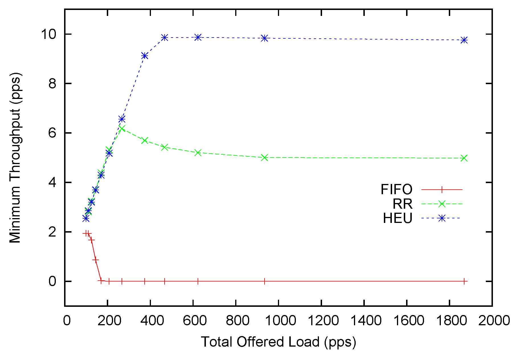
4.2. Performance with Poisson Arrivals
The effectiveness of our heuristic scheduling rules is examined next. In this subsection, we test our scheduling scheme with Poisson packet arrivals. MASON (A multi-agent simulation environment) [
21] is chosen to be the simulator used, because it is a fast discrete-time Java-based simulator. In this simulation, we simply model the behavior of a queuing system. We are interested to see whether, in an isolated environment, our scheduling scheme can perform better than other existing scheduling schemes. A more extensive and more realistic simulation is done in
Section 5, so as to evaluate the overall performance of our scheduling scheme with all network factors considered.
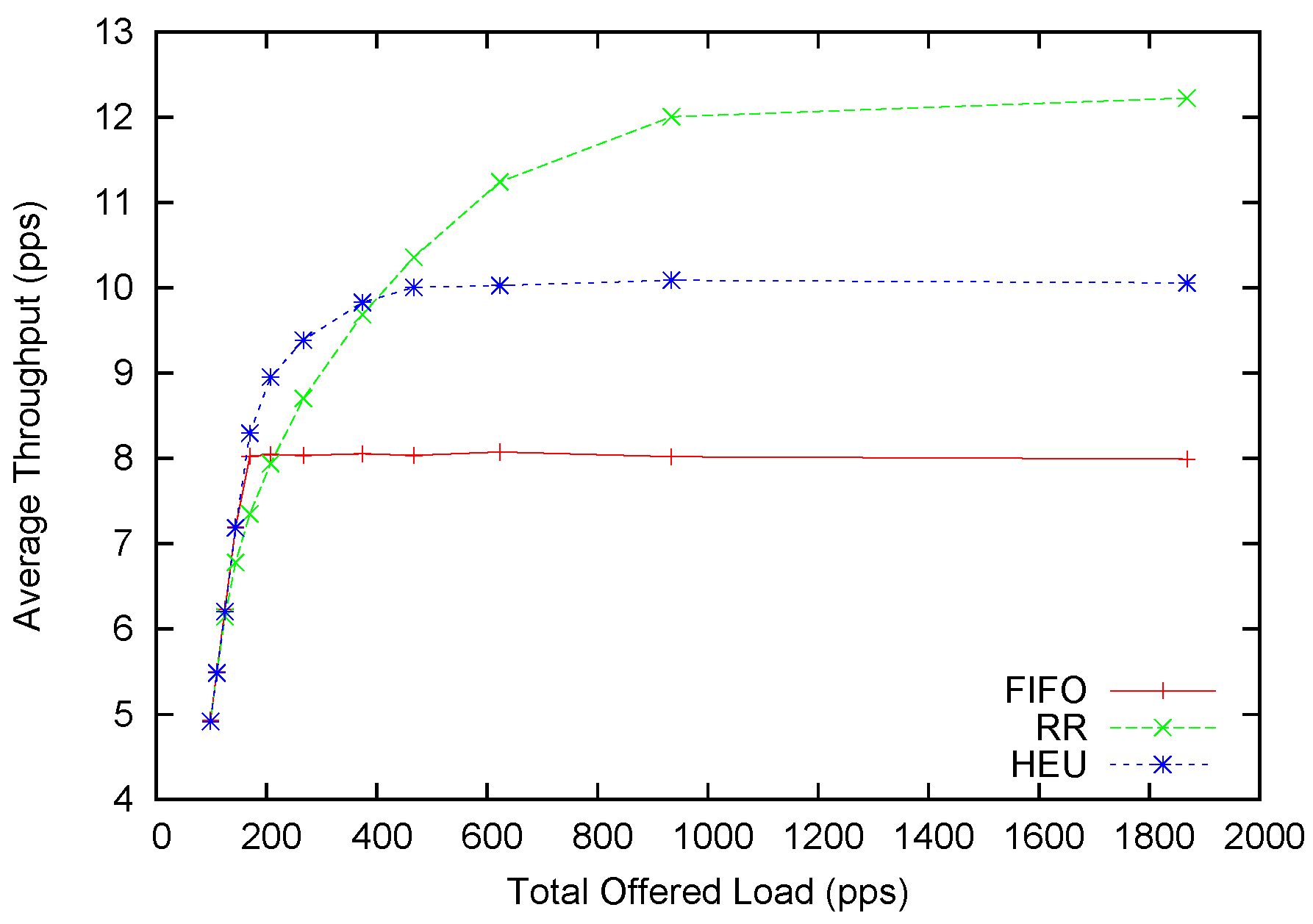
Two frequently used scheduling schemes are taken as the comparison group. One is FIFO-based, and the other is round-robin-based. Basically these two-packet scheduling schemes cover all existing literature on network coding protocols. In the FIFO-based scheduling scheme, all packets arrive at a single queue, each with a tag denoting which flow it is coming from. When the node obtains the right to transmit, the first packet in the queue is dequeued first, and it checks sequentially in the queue for coding-possible packets. On the other hand, the round-robin-based scheduling scheme maintains multiple queues, each for a flow. The scheduler then polls these queues in a round-robin fashion. This scheme overcomes the problem in the FIFO-based method that a busy flow can crowd out all other flows.
Among all generated coding graphs using the baseline parameters (
cf.
Table 1), the one that corresponds to the median processing time is used in this experiment. This choice guarantees that the generated coding graph is neither too plain, nor too complex. In the baseline test bench, a total of 20 flows are present. The total offered load is 1868 packets per second (pps), with the minimum flow being 48 pps and the maximum being 282 pps. Each simulation is run for 60 s (time in simulation). The average throughput and minimum throughput among all flows are sampled from the end of the 10th second until the end of the simulation. After 10 s, the system has already stabilized, so we choose to measure the throughputs from 10 s onward to the end of the simulation. All experiments are done with 10 different random seeds, and the average is plotted in
Figure 7 and
Figure 8.
Figure 7.
Average throughput performance with Poisson arrivals.
Figure 7.
Average throughput performance with Poisson arrivals.
In the static version of this scheme, a round-robin-based scheduling scheme requires 1198 transmissions to clear the queued packets. However, our static solution requires only 1010 transmissions. This is almost a 20% improvement.
Figure 8.
Minimum throughput performance with Poisson arrivals.
Figure 8.
Minimum throughput performance with Poisson arrivals.
In the dynamic case, the average throughput improvement is not as significant. We scale the offered packets with a multiplier and generate different offered loads. The distribution of service rates follows a Poisson distribution with mean service time as 100 packets per second. It is observed that our heuristic scheduling scheme (HEU) can outperform round-robin (RR) when the offered load is below 400. This is four-times the transmission capacity. The maximum improvement can reach 13%. This amount is smaller than the 20% promised in the static form. This is generally because our heuristic scheduling method balances between better performance and higher anomaly tolerance. Only if we can always stick to the optimal scheduling scheme can we achieve the highest performance improvement. However, a fixed scheme cannot adapt to the dynamic network conditions. With the introduction of probabilistic scheduling and the allowance mechanism, we achieve adaptability to network contingencies at a small cost of potential performance gain. When the offered load continues to rise above 400, RR provides higher average throughput as compared to HEU. At the same time, we turn to
Figure 8 for more insight about this underperformance. One can soon discover that the minimum throughput of HEU is slightly below 10 pps, while the average throughput is slightly above 10 pps. This indicates that our scheme achieves the
de facto fairness by allocating almost equal-throughput channelsfor each flow. The RR scheme can provide around 12 pps average throughput, but its minimum throughput is only around 5 pps. This is most conspicuous for the FIFO scheme where the minimum throughput is plainly zero. In fact, from the 250 pps offered load and above, HEU can provide better fairness than RR. However, it only starts to underperform in terms of average throughput after 400 pps.
To sum up, when the network is not severely saturated (e.g., the offered load is four-times higher than the processing speed), our heuristic scheduling scheme for the dynamic case can provide higher average throughput across all flows. At the same time, our scheduling scheme constantly provides better fairness than other scheduling schemes. It overcomes the crowd-out effect of other scheduling schemes when the offered load is too high, and some flows may suffer for low or even zero throughput.
5. Evaluation
In this section, we evaluate our work in a sophisticated network environment, specifically, an environment with upstream/downstream nodes, contentions and interferences. We first tune our heuristic scheduling scheme to counter the adverse effects that we may encounter in real networks. Then, the tuned scheduling scheme is tested in Qualnet simulations, where a set of network topologies with multiple nodes are constructed. The evaluation results would reveal that with some tailored packet scheduling algorithms, we can, for example, improve the fairness among flows without severely impacting overall throughput. If fairness is of less importance in some scenarios, one can modify the ideas underlying our algorithm to improve throughput. One simple idea is to shift some quota from flows with less coding degree to flows with higher coding degree, as in the generate-quota algorithm.
There are mainly three assumptions in the evaluation of our heuristic scheduling scheme, as described in the last section. However, they are not immediately valid in real network settings.
- (1)
The offered load of each flow is known and fixed.
- (2)
The transmission capacity of each node is known and fixed.
- (3)
The arrival of packets follows the Poisson process.
Therefore, we have to make adjustments to fit the scheduling scheme in a real protocol. Hence, we designed DPSA (dynamic packet scheduling algorithm), on top of the routing protocol proposed in [
22]—SCAR. SCAR is a routing protocol based on DSR (The dynamic source routing protocol for multi-hop wireless ad hoc networks) [
23]. Routes are selected in an on-demand fashion, and source routing is used to navigate packets through the network. SCAR is able to discover coding opportunities and compare potential throughput gain among multiple paths.
The first adjustment is the design of a cross-layer channel. Using this channel, the application layer can give hints to the offered load to lower layers. Consider a flow with three nodes, S, I and D. The offered load information is directly available through the cross-layer channel in Node S. However, the offered load in Node I is usually smaller, because Node S may not have processed all packets from the flow. At the same time, some packets may be dropped due to queue overflow.
Therefore, the second adjustment is the delivery of offered load information from the upstream nodes to the downstream nodes. An upstream node calculates the offered load for a downstream node by subtracting the amount of packets dropped from its own offered load, periodically. This delivery of information is encoded in the source routing header.
The third adjustment is the introduction of changing transmission capacity. This is a critical value used in the heuristic scheduling scheme. Overstating this value will generally lead to unfair scheduling, and understating this will lead to lower throughput gain. In our protocol, this value is measured as the number of packets processed per second, averaged over a window of 5 s. Therefore, it can reflect changes in the network condition, but filter out unnecessary noises.
In the following text, we test our scheduling method in two types of topologies. The first one is specially designed to contain plentiful coding opportunities. The second one is a randomly generated mesh network, which resembles real-world ad hoc networks. In this topology, the amount of coding opportunity is intermediate. In topologies where coding opportunities are rarely seen, our scheduling method is retrograded to a round-robin scheme and, thus, is omitted in this analysis.
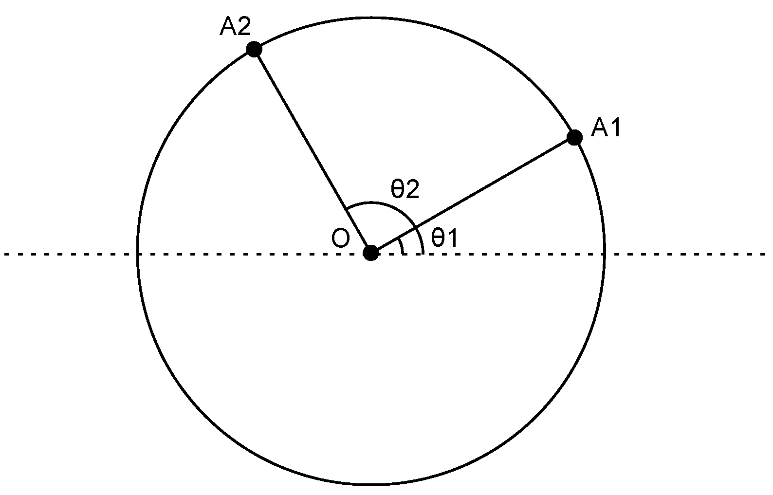
5.1. Experiment 1
We choose a circle topology in Experiment 1, as shown in
Figure 9. First, we fix a central node
O and the radius
r of a circle. Then, we randomly generate an angle
between zero and 360. Node
is added on the circle, such that the line segment that connects
and
O intercepts the positive axis with an angle
. This process is repeated
N times until
N nodes are added on the circle. The traffic patterns are randomly generated as long as the source node and the destination node are not in transmission range (
R) of each other [
19]. A total of
e flows are selected, and all of these flows use Node
O as the intermediate node. The experimental parameters are described in
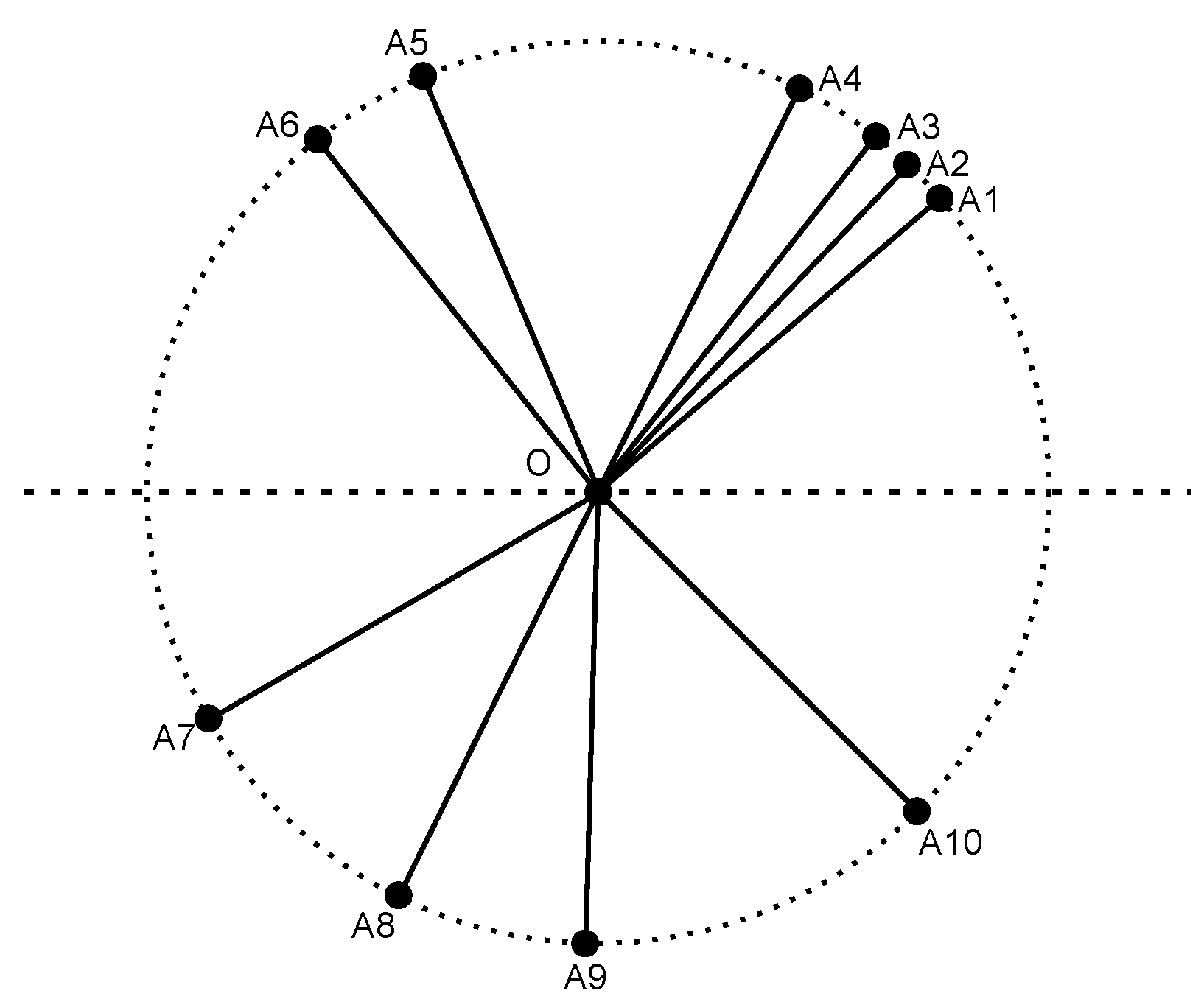
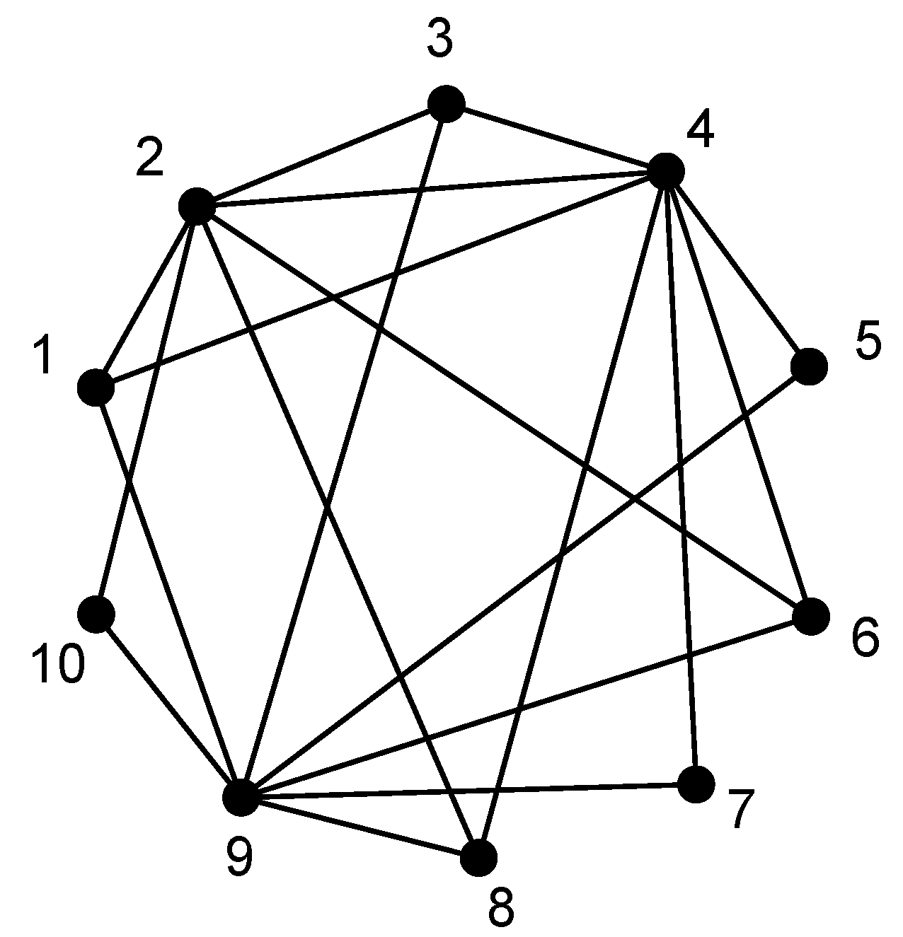
Table 2. The generated topology and the coding graph are shown in
Figure 10 and
Figure 11, respectively. For simplicity, we manually choose Node
O as the intermediate node for all flows.
Figure 9.
A topology where source and destination nodes are on the same circle.
Figure 9.
A topology where source and destination nodes are on the same circle.
Figure 10.
The generated topology for Experiment 1.
Figure 10.
The generated topology for Experiment 1.
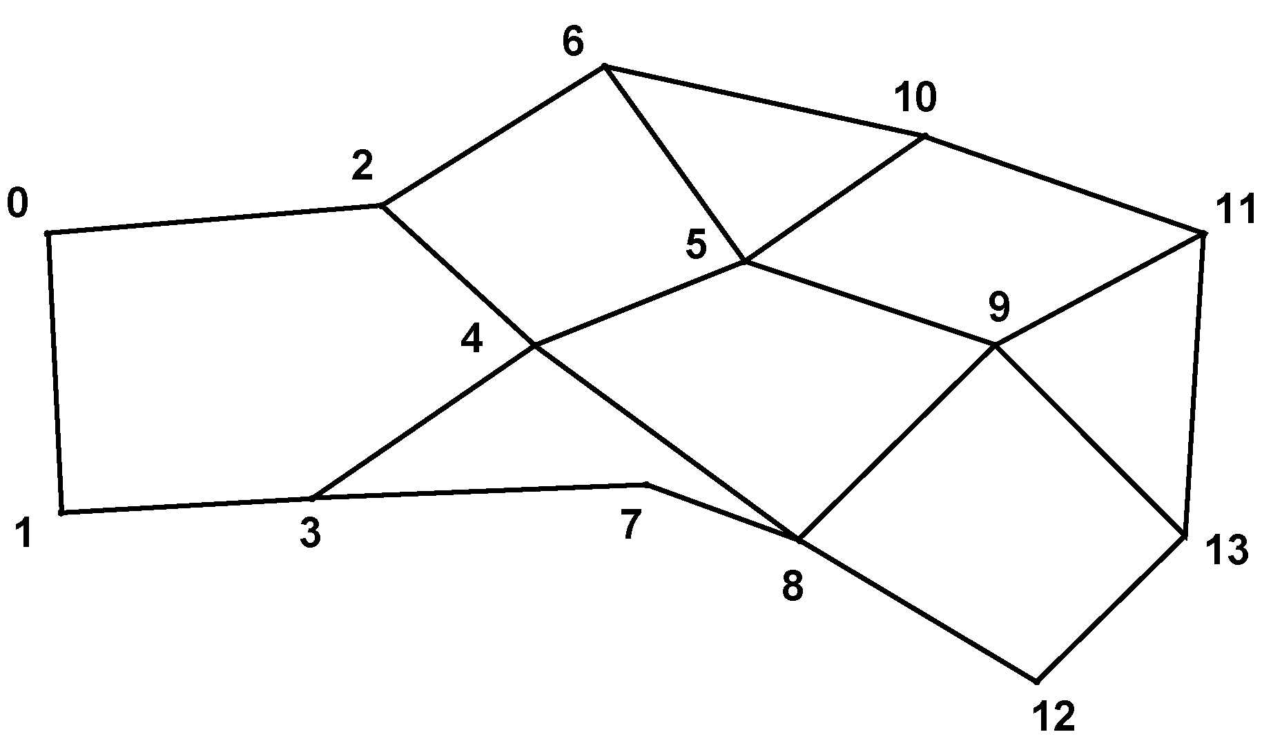
Figure 11.
Coding graph at Node O in Experiment 1.
Figure 11.
Coding graph at Node O in Experiment 1.
Table 2.
Experiment 1 parameter settings.
Table 2.
Experiment 1 parameter settings.
| Parameter | N | e | r | R |
|---|
| Value | 10 | 10 | 100 | 150 |
The comparison group is chosen to be SCAR [
22], which uses round-robin scheduling. In this experiment, each simulation is repeated 10 times with different random seeds, and the measurements are averaged.
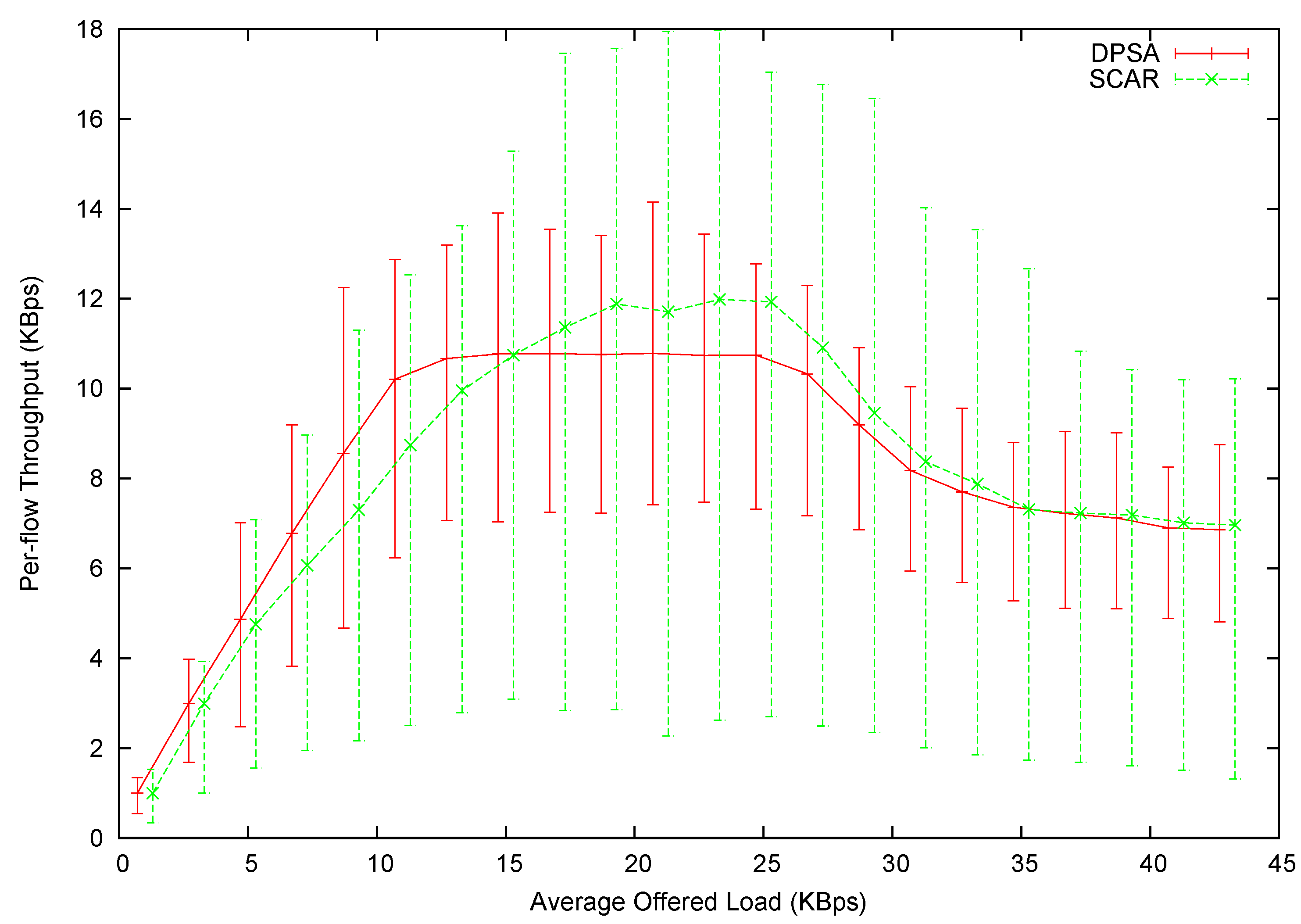
The per-flow average throughput is shown in
Figure 12, with the error bars showing the minimum and maximum per-flow throughput. Note that the points are slightly shifted along the
x-axis for visual clearance. The exact
x value should be the mid-point between each pair of data points. It is observed that DPSA can initially provide higher throughput than SCAR. This is because DPSA systematically schedules the packets to be coded together, minimizing the number of transmissions to clear packets in the queue. In addition, DPSA almost provides a straight line connecting the zero point to its highest achievable throughput. On the other hand, the curvature of the SCAR line is much higher.
Figure 12.
Per-flow throughput in Experiment 1.
Figure 12.
Per-flow throughput in Experiment 1.
However, DPSA’s maximum throughput level is lower than DPSA’s. This happens when the network is fully saturated, i.e., the transmission capacity of the router node is smaller than the offered load. DPSA schedules packets in an order first to guarantee fairness. In terms of the coding graph, DPSA intentionally shifts transmission capacity from those well-connected vertices to the ones that have fewer neighbors. The result of this shifting is conspicuous. The throughput span is significantly narrowed, meaning smaller variance and better fairness. DPSA can fairly allocate bandwidth to all flows: the minimum throughput among all flows is roughly 70% of the average throughput. On the other hand, some flows receive only around 20% of the average throughput in SCAR.
As the offered load continues to rise, the average throughput of both protocols declines. This is mainly because of MAC-layer contention of source nodes. The router node has decreasing transmission capacity, because the media is more often occupied by the source nodes. In fact, we have designed a congestion control mechanism for our protocol. Such a congestion control mechanism can detect the congestion and reduce the amount of packets sent by the source nodes. Therefore, our protocol can maintain the highest throughput, even when an offered load further increases. However, this paper emphasizes the importance of a packet scheduling scheme, so this part is omitted intentionally.
5.2. Experiment 2
In this experiment, we take a random topology to mimic real-life
ad hoc networks. The topology is shown in
Figure 13. We randomly choose 10 S-Dpairs and generate traffic according to a randomly-generated ratio.
Figure 13.
The topology of Experiment 2.
Figure 13.
The topology of Experiment 2.
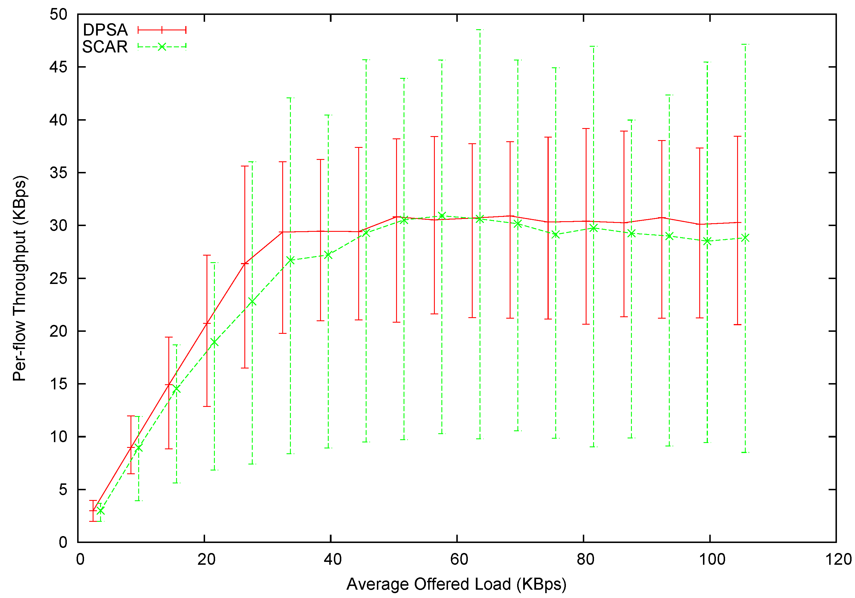
In
Figure 14 we have plotted the average throughput
versus the average offered load. In this experiment, we can still observe that DPSA provides higher throughput than SCAR when the network is not yet saturated. However, the difference in the average throughput of a saturated network almost vanishes. This can be explained by the cascading effect: In Experiment 2, most flows have more than two hops. The scheduling decision made at one node can affect the offered load of the next. Without proper planning (as in round-robin scheduling), a great proportion of packets are discarded along the way. This is a great waste of bandwidth, which effectively decreases the maximum throughput achievable by the round-robin scheduling. This can be explained by the cascading loss effect. In a flow with more than one hop, the scheduling decision made at an upstream node can affect the offered load of the immediate downstream node. Without proper planning (as in round-robin scheduling), the mismatch in each hop would waste a certain amount of bandwidth. The more hops one flow has, the more severe becomes bandwidth loss. This is referred to as the cascading loss. A great proportion of packets can be discarded this way, which effectively decreases the maximum throughput achievable by the round-robin scheduling. Also note that DPSA managed to schedule packets more fairly, and the scheduling maintains a good linkage between upstream nodes and downstream nodes, minimizing the cascading effect. In addition, the significant decrease of throughput, as seen in Experiment 1, is not present. This is simply because the MAC-layer contention is not as severe as in Experiment 1’s topology.
Figure 14.
Per-flow throughput of Experiment 2.
Figure 14.
Per-flow throughput of Experiment 2.
6. Conclusions
In this paper, we have highlighted an area of a problem that has long been neglected—the packet scheduling scheme with network coding enabled. The problem is tackled first in a simplified and static version. With our scheduling method, intermediate nodes can clear packet queues faster, and the scalability of the algorithm is also tested. The findings are then applied to the dynamic form of the scheduling problem, where we consider multiple queuing systems. Though it is hard to analyze the system, we proposed a heuristic scheduling method addressing the challenges posed by a dynamic system. The solution to this dynamic problem is then incorporated into a routing protocol. Simulation results for this routing protocol reveal that with proper scheduling, we can have better control over the fairness of the network. When fairness is not a concern, one can easily adapt our protocol to put more emphasis on those higher coding gain pairs to improve throughput.


