1. Introduction
The Internet of Things (IoT) will reach out into everyday objects and environments by connecting tiny embedded computers that can perceive their environment by means of sensors. It is anticipated that by 2020, tens of billions of such embedded devices will be connected to the Internet—one order of magnitude larger than the number of computers connected to the Internet today. In the IoT, the state of the real-world is available online and in real-time and can be combined with existing data and services in the Internet to realize a broad range of innovative and valuable applications such as Smart Cities, Smart Grids, or Smart Healthcare.
While research has recently focused on how to extend the Internet and Web Protocols—most notably IP and HTTP—into these resource-constrained wireless embedded devices, the question of how to represent sensor data in the IoT in an open way such that it can be efficiently searched and combined with other data is still open. A particular challenge therein is the highly dynamic nature of sensor output, resulting in huge real-time data streams being generated by embedded devices.
This paper makes a contribution towards enabling open and scalable search in the Internet of Things by leveraging concepts known from the Semantic Web. The latter introduces a data format known as RDF (Resource Description Framework) to encode arbitrary facts as subject-predicate-object triples that can be stored in special database systems known as triple stores. Using the SPARQL query language, queries over triples stored in such databases can be formulated and executed. A growing body of world knowledge (e.g., including the information in Wikipedia) is being encoded into such RDF triples and queries across different domains can be posed with SPARQL.
Our aim is to encode sensor data as RDF triples such that joint queries over sensor data and existing world knowledge encoded as RDF triples can be posed using SPARQL. A fundamental challenge therein lies in the fact that RDF databases and SPARQL have been designed for static or slowly changing sets of triples, yet sensor output is highly dynamic. We tackle this problem by introducing prediction models that allow estimating the current output of sensors without requiring the sensors to stream all their output values into the IoT. In this paper we show how to encode such prediction models as RDF triples and how to evaluate those prediction models using SPARQL queries.
We first summarize the state of the art and its limitations in
Section 2 before introducing our approach in
Section 3. The core contribution of the paper can be found in
Section 4, describing how to encode predictions models in RDF and how to evaluate those models by means of SPARQL queries. Related work is discussed in
Section 5 before concluding the paper in
Section 6.
2. Towards a Semantic IoT
A central issue of many of today’s sensor and actuator networks is that they use proprietary protocols and data formats and are typically locked into unimodal closed systems. For example, motion detection sensors in a building may be exclusively controlled by the intrusion detection system. Yet the information they provide could be used by many other applications, for example, placing empty buildings into an energy-conserving sleep mode or locating empty meeting rooms. Unlocking valuable sensor data from closed systems has the potential to revolutionize how we live. To unleash their full potential, access to sensors should be opened such that their data and services can be integrated with data and services available in other information systems, facilitating novel applications and services such as Smart Cities, Smart Homes, Smart Grids, etc. Below we briefly summarize recent efforts to realize an open Internet of Things, where sensor data are published in open formats using standardized protocols.
Internet Integration of IoT Devices Regarding proprietary protocols, there is a trend towards standardization and two protocols are gaining momentum: 6LoWPAN and CoAP. 6LoWPAN [
1] is a light-weight IPv6 adaptation layer allowing sensors to exchange IPv6 packets with the Internet. CoAP (Constrained Application Protocol [
2]) is a draft by IETF’s CoRE working group, which provides a light-weight alternative to HTTP using a binary representation and a subset of HTTP’s methods (GET, PUT, POST, and DELETE). For an exhaustive discussion of 6LoWPAN, CoAP, and RESTful services, we refer the reader to [
3].
6LoWPAN in combination with CoAP allows sensor data of IoT devices (e.g., temperature readings) to be queried or to trigger actuations of IoT devices (e.g., to switch on a light or to increase heating of a room) from the Internet as these devices provide RESTful web services [
4]. Such services can either return data in different representations (e.g., plain-text or HTML) using standard HTTP content negotiation or trigger actions (e.g., by sending a POST request with new settings).
For instance, an application could query the state of a sensor by sending a GET request to the sensor (e.g.,
http://ipv6-address-or-dns-name/room-sensor). The sensor replies with the sensor’s value encoded in a—possibly proprietary—encoding such as plain text (e.g.,
occupied) or any format the sensor supports.
Data Format While protocols such as 6LoWPAN and CoAP solve the basic Internet integration and interoperability issues, a problem is still the data format used by IoT devices. The variety of formats and their lacking integration hinder IoT application development. In previous work [
5], we presented how Semantic Web technologies (
i.e., RDF [
6], W3C’s Resource Description Framework) can serve as the melting pot that amalgamates real world data and data from the Internet to realize such novel applications. RDF is a Semantic Web standard to describe statements in terms of triples composed of a subject
S, a predicate
P and an object
O. While
P is a reusable resource in terms of a URI,
S can be either a URI or a blank node,
i.e., an anonymous resource without a URI and thus no accessible representation, and
O can be a resource, a blank node, or a literal (e.g., a string or number). Through the reuse of resources, RDF builds a graph where
S and
O are nodes and
P are directed edges from
S to
O.
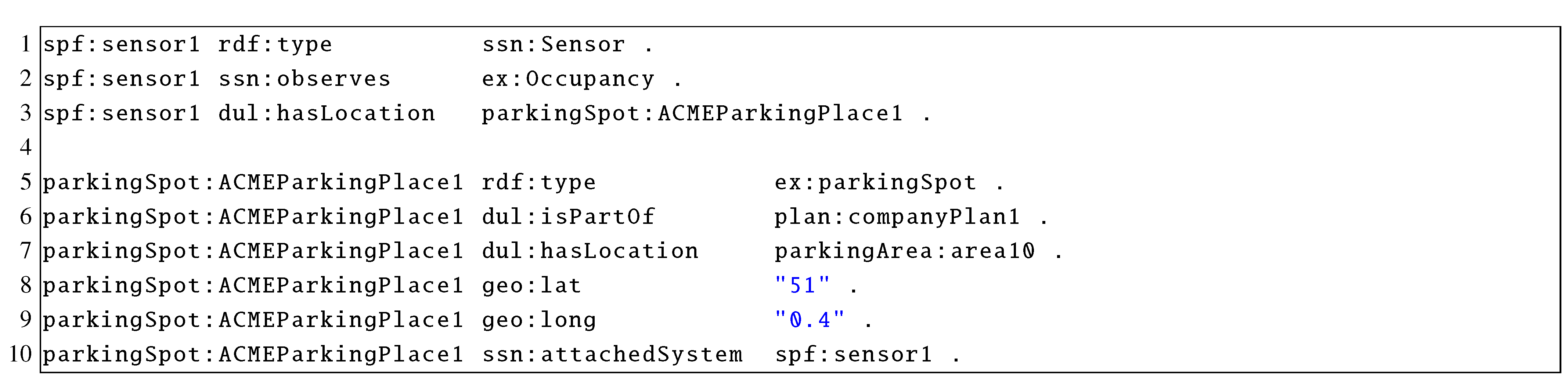
Figure 1.
Exemplary description of a parking spot occupancy detection sensor.
Figure 1.
Exemplary description of a parking spot occupancy detection sensor.
As an example,
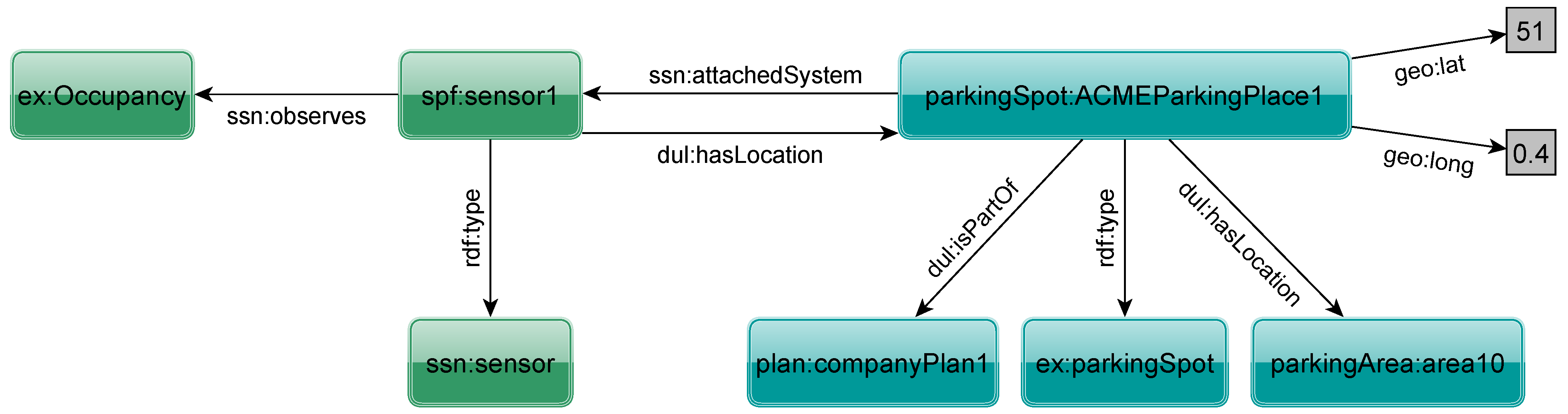
Figure 1 presents part of an RDF description of an occupancy detection sensor located in a parking spot. The triples state that a particular object is a sensor (Line 1) measuring occupancy (Line 2) located in a particular parking spot (Line 3). The parking spot (Line 5) belongs to a specific company (Line 6) and is located in a given area (Line 7) with a given geographical location (Lines 8 and 9) and has the previously described sensor attached (Line 10). The resulting RDF graph is shown in
Figure 2. This shows how a sensor could provide an unambiguous machine-understandable self-description.
The actually used URLs are in principle arbitrary, but to maximize interoperability and usefulness, one should use well-known and frequently used vocabularies. An important vocabulary for the IoT domain is the
Semantic Sensor Network Ontology (SSN, [
7]). It supports the description of the physical and processing structure of sensors.
Sensor Search With 6LoWPAN, CoAP, RDF, and the appropriate vocabularies such as SSN, important interoperability issues are solved conveniently. However, to implement large-scale, Internet-wide applications, the ability to find sensors having certain properties or current states is of vital importance. Consider the use case of finding an available meeting room in a certain area that is already heated in order to save costs. Such an application would have to (i) locate the service URLs of sensors that measure temperature in this region; and (ii) query the current value of the sensors. While the first task relies on slowly changing, nearly static metadata about a sensor, the second one has to deal with frequently changing sensor readings. Frequently querying the value of sensor is problematic for a number of reasons (e.g., because of energy depletion of battery-operated devices or consumption of scarce bandwidth resources in wireless multi-hop networks).
To solve these problems, one could use technologies from the Semantic Web community such as SPARQL [
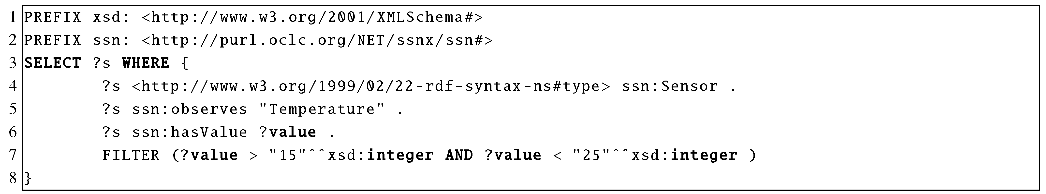
8], which is the standardized query language for RDF with a similar syntax as SQL. An example query is shown in
Figure 3: This query asks for all temperature sensors with a current value between 15 °C and 25 °C. The first two lines contain namespace prefix declarations to allow using abbreviation in the query for better readability. The result set includes every resource that matches the variable
?s (Line 3). Lines 4–6 specify atomic triple patterns where known URIs and literals of triples are specified and unknown ones are marked as variables (prefixed by ?). The results of the query must match with the RDF graph (in this case the type must be ssn:Sensor, it must observe the property temperature, and have a value of
). Line 7 removes results that are not in a given range (a so-called
range query). In addition to these conjunctions, also disjunctive queries can be expressed using the UNION keyword.
Figure 3.
Example of a SPARQL query.
Figure 3.
Example of a SPARQL query.
Limitations of Existing Approaches While this approach works well for nearly static metadata, it is not well suited for frequently changing sensor values. Each IoT device would have to publish all sensor values such that they can be indexed by Semantic Web search engines. These engines would be required to crawl and index all sensors with a high frequency in order not to miss any important updates. Clearly, this is not a scalable solution. Therefore, we next introduce an approach to address this problem.
3. Approach
To enable scalable search for sensors reading a given value in the Internet of Things, communication with the sensor nodes needs to be minimized. To this end, we had earlier introduced an approach called
sensor ranking [
9], where sensor nodes autonomously compute a prediction model based on past sensor data. Such models allow estimating the probability that the sensor reads a given value at a given (future) point in time. Instead of downloading raw sensor time series, a search engine would infrequently download those prediction models from sensors. To answer a query for sensors currently reading a given value, the search engine would execute those previously indexed prediction models to obtain a ranked list of sensors that is sorted by decreasing probability of a sensor currently reading the sought value. This result set lists sensors first that have the desired value with high probability. To verify this, the actual value must be obtained from a device by requesting the current value using a device’s URL. This approach substantially reduces the amount of communication and thereby also the time needed to find a given number of matching sensors.
In our previous work, we used custom representations of those prediction models, which made the integration with existing search engines difficult. The contribution of the present paper therefore lies in defining an open and flexible representation to represent those prediction models (in RDF) such that they can be queried with existing query engines, notably SPARQL, as detailed in the subsequent section.
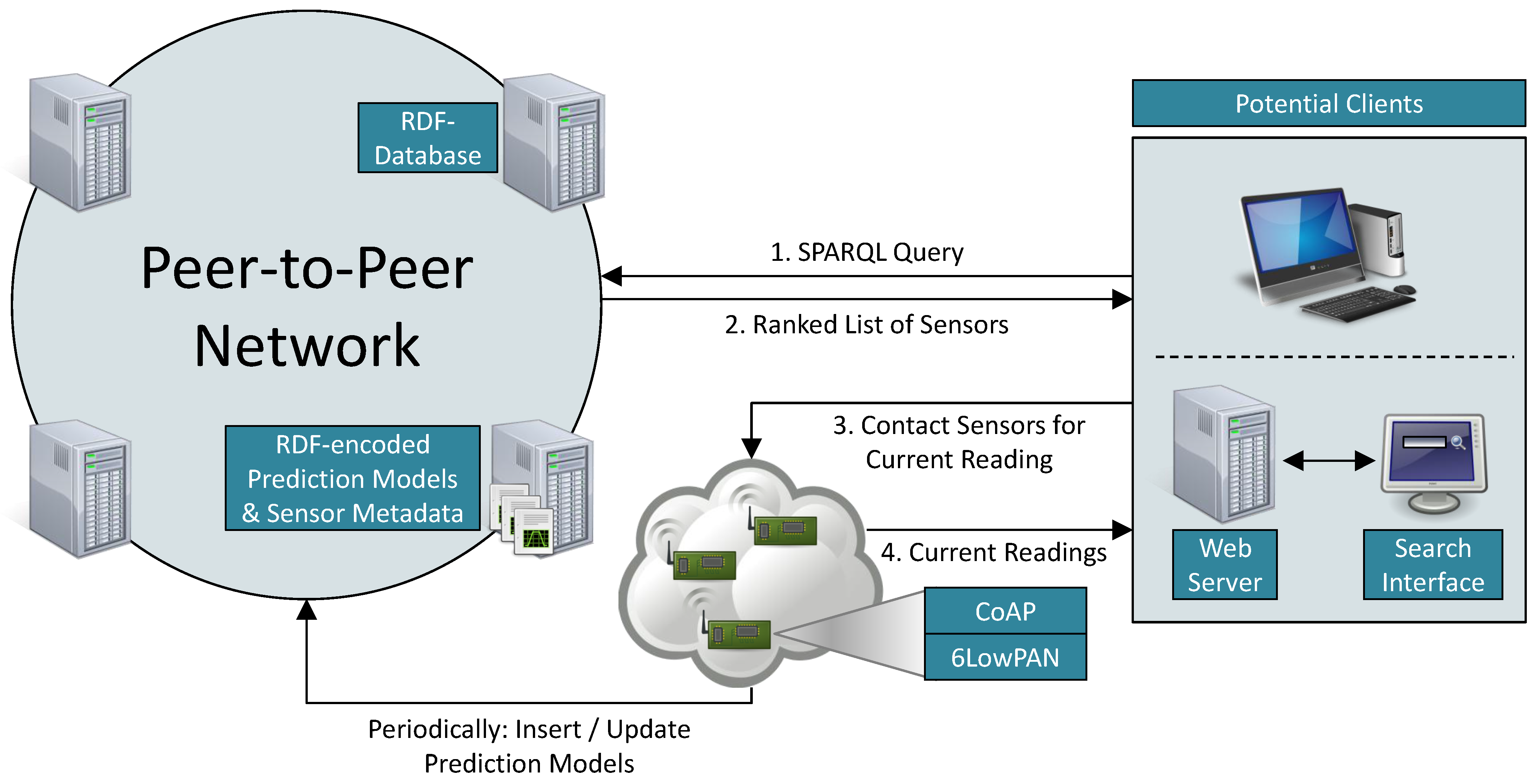
Figure 4 depicts the envisaged overall architecture of our system. IoT devices (
i.e., sensors and actuators) are connected to the Internet via 6LowPAN and expose their services using CoAP. These web services can return current sensor readings, a description of a device’s properties, or its prediction models. We assume that these data are encoded as RDF triples. These are stored in a RDF database that exposes a standard SPARQL endpoint via HTTP, which is used by clients to send queries. The RDF database returns a ranked list of sensors, and the clients then contact device after device and obtain the current sensor reading until a device with the desired value is found.
To make this work on an Internet scale, a distributed RDF database should be used but is not required by our approach. A number of scalable peer-to-peer-based RDF databases have been proposed (e.g., RDFPeers [
10], Atlas [
11], 3RDF [
12], GridVine [
13], or DecentSparql [
14]) that distribute RDF triples amongst a—potentially huge—number of peers. Such databases can be used without changing our system as long as SPARQL is fully supported (which is to the best of our knowledge currently only the case for DecentSparql [
14]). In such a scenario, even parts of the IoT (e.g., embedded computers, routers and other hardware resources), which are most of the time rarely used or even idle, could be part of such a peer-to-peer network and thus the IoT would even provide self-growing storage and query capabilities.
Figure 4.
Overall search architecture.
Figure 4.
Overall search architecture.
A fundamental design decision underlying our work is how to represent sensor readings. We decided to represent the output of a sensor as a typically small set of discrete, unordered states. This is motivated by the observation that typical end users are typically not interested in the raw and often noisy output time series of physical sensors, but in high-level descriptive states. For example, room occupancy can be measured by a passive infrared sensor that triggers an interrupt whenever the warm body of a person moves in the room. However, also other changes in the heat signature (e.g., caused by changing sunlight intensity) may trigger the sensor. This results in a noisy time series of movement events that may be interesting for an expert. However, an end user is typically interested in knowing if the room is occupied or free. Therefore, we would model the output of a room occupancy sensor by two discrete states {free, occupied}, assuming that the actual raw output time series of the physical sensor is preprocessed and potentially fused with the output of other sensors in order to obtain those high-level states.
Two further advantages result from this approach. Firstly, in contrast to high-level states, raw sensor data may reveal privacy-sensitive information. For example, if a camera is used to measure the occupancy of the room, the raw camera image may reveal the identities of persons in the room, whereas a high-level state occupied does not.
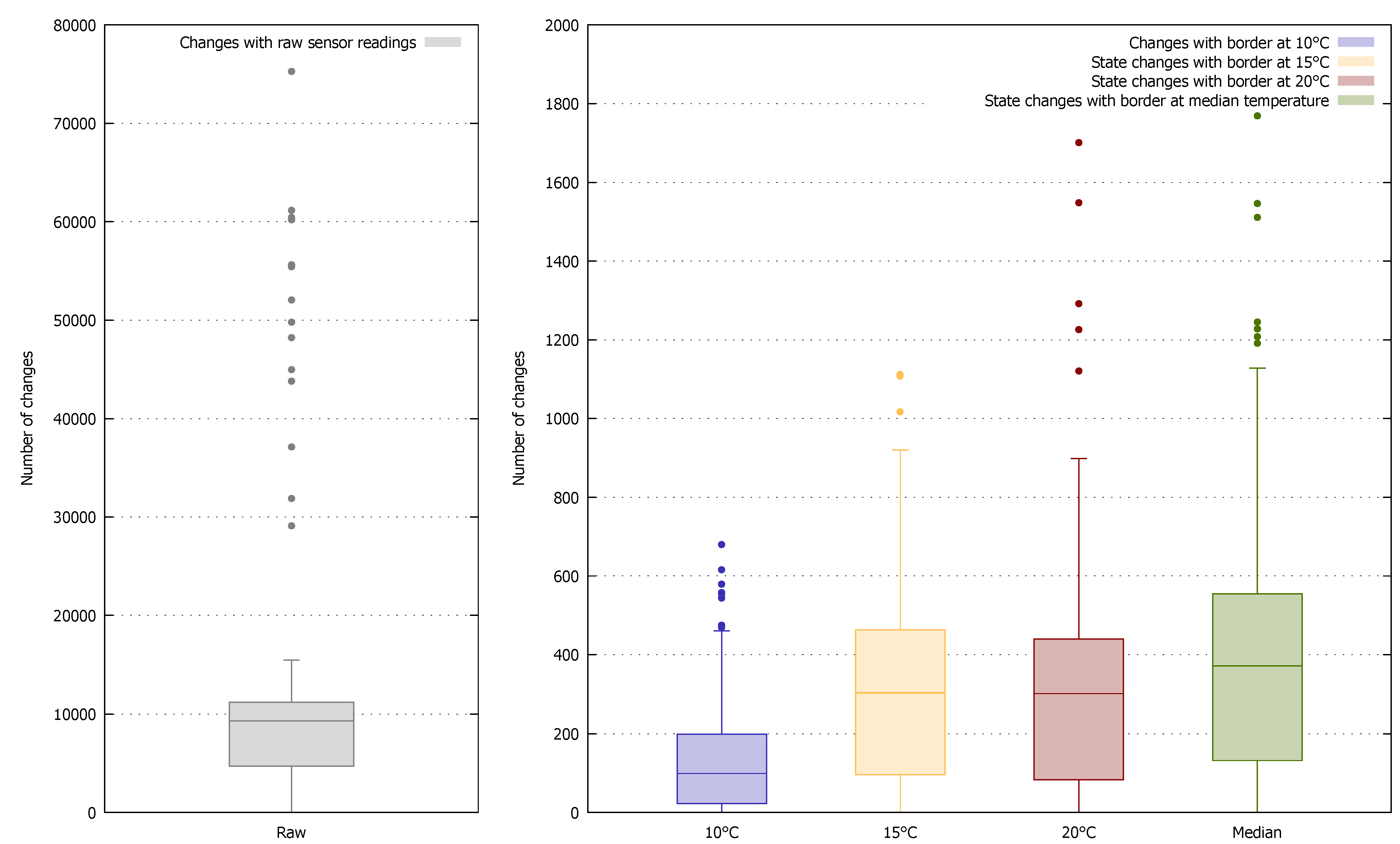
Secondly, compared with a time series of raw sensor data, a time series of high-level states is often much more compact due to the smaller amount of information contained in the latter. We illustrate this in
Figure 5, which shows the number of changes in consecutive raw sensor readings from over 700 temperature sensors (≈8.5 million readings) of the real-world deployment of the Smart Santander project (EU FP7 project SmartSantander:
http://smartsantander.eu) during a period of about one year. The median number of changes among all sensors is close to 10,000. On average 72% of consecutive sensor readings differed. In the right plot we took the same temperature readings and classified them as either
cold or
warm. We used four different borders for classification, namely 10, 15, and 20 °C as well as the median reading of each sensor to categorize its readings. Note the different scale on the y-axis. The number of changes between consecutive states is reduced by a factor of 25–100 depending on the used border. Hence, if sensor nodes only report changes in states, a considerable amount of resources can be saved.
Figure 5.
Boxplots of number of changes of temperature sensor readings respectively states.
Figure 5.
Boxplots of number of changes of temperature sensor readings respectively states.
4. Semantic Probability Models
In this chapter we introduce our approach to model the states of sensors and prediction models for these states with the help of RDF. We will incrementally add new parts to the model to explain step by step what required and optional elements can be used and how they work together.
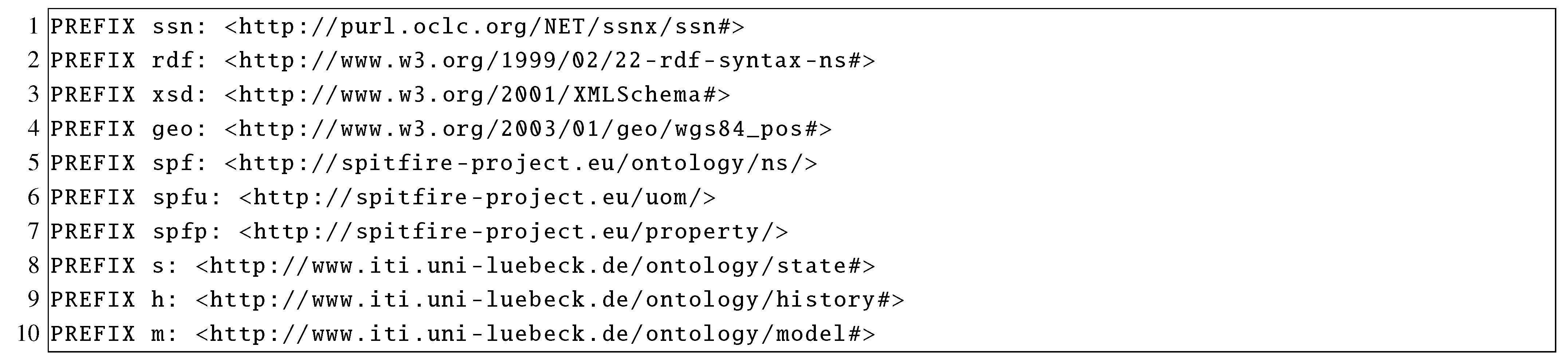
All namespaces are abbreviated to keep the graph small and readable. The used prefixes are shown in
Figure 6 as one would define it for SPARQL queries. Typically, the URLs are pointing to web resources where further information about the semantics can be found. We omit these namespace definitions in subsequent SPARQL-queries for better readability and clarity. In the figures all subject and object resources are shown as rectangles with rounded corners. Newly introduced resources are colored while the already known elements are grayed out. Literal objects are rectangles without rounded corners with a grey background. Instead of showing the XML schema types of the literals, we encoded the format with the help of the frame. A solid frame indicates a number literal, a dotted frame a string literal and a dashed one time or date types. Edges are the predicates and are directed from the subject to the object.
4.1. Base Sensor Structure
As a base for our approach we use the SSN Ontology [
7], which is also used in different other research projects [
5,
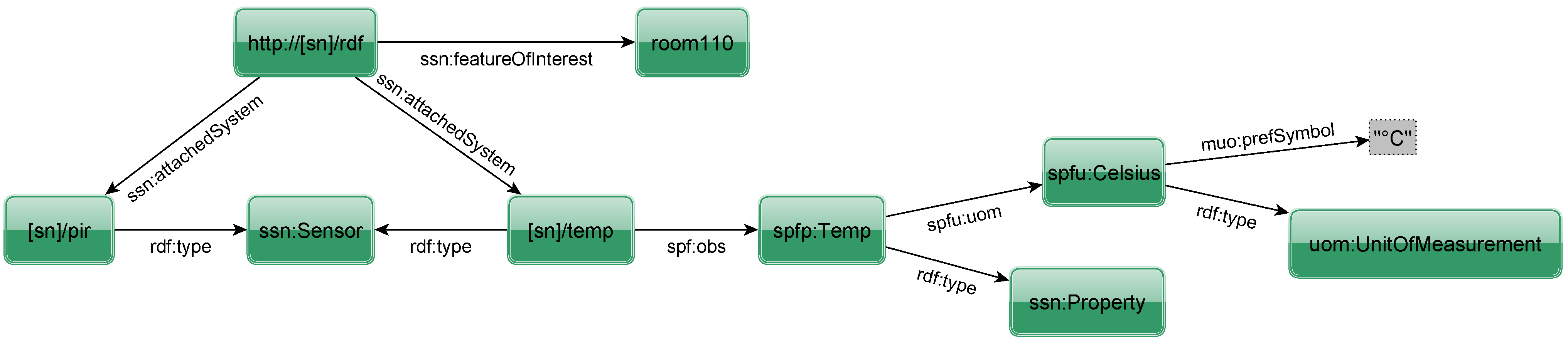
15]. It allows modeling, among other concepts, sensor nodes and their capabilities. A cutout of a resulting RDF graph, which we use as a base for our model, can be seen in
Figure 7. The sensor node is given by the RDF node
http://[sn]/rdf where
http://[sn] denotes the IPv6 address of this specific node (which is shortened to
[sn] in other nodes for clarity). The suffix points to a resource describing the sensor node in RDF. In the Internet of Things, sensor nodes will be deployed to observe the state of entities. This is modeled by the property
featureOfInterest. The other two triples specify the available systems on that node using the property
attachedSystem. Hence, in our example the sensor node is placed in room 110 and has two attached systems of type
sensor. The URI of the leftmost resource suggests that it is a passive infrared sensor (PIR), which is not further considered in the example. The other system is a sensor that
observes the physical property
Temperature in units of °C.
Figure 7.
RDF to describe sensor node and attached sensors.
Figure 7.
RDF to describe sensor node and attached sensors.
4.2. States of Sensors
As argued before, we are not interested in raw sensor readings but in high-level states. Hence, we have to define a set of states a sensor can measure. Thus, instead of storing a raw value such as 21 °C, a temperature sensor should output the state
warm. However, different people have different views on what warm means. A resident in the city of Lübeck (North of Germany) might feel 15 °C as warm whereas a resident of Santander (Spain) is still freezing. Hence, an arbitrary number of states for a concept such as warm can exist in parallel. Out of these, suitable states can be selected for a sensor depending on its location.
Figure 8 shows the definition of the states
warm and
cold. Each state defines a range by means of a lower and upper bound on raw sensor readings. In the example, a sensor is in state cold if it measures a temperature between minus infinity and 20 °C. Everything from 20 °C upwards is considered a warm state. While the lower bound is inclusive, the upper bound is exclusive. If both bounds would be inclusive, the state to choose for 20 °C would be ambiguous. Otherwise, if both bounds are exclusive, no state would exist for that temperature.
Figure 8.
RDF to describe sensor states.
Figure 8.
RDF to describe sensor states.
Additionally, a state can have an arbitrary number of descriptive terms. This allows for easy textual search for a state. Both states are of type TempState, which is in turn a subclass of State. The TempState is referenced by the physical property to show that all children of that element are possible outcomes of that physical property; e.g., a warm-state is reasonable for temperature but not for humidity. With the property possibleState to a state instance, a sensor can specify which warm-state is used by him. Although we think that a few states would suffice for a physical property, it is up to the user to define the granularity of the states. Thus, e.g., for temperature, even one degree or smaller steps are possible. Hence, almost continuous scales can be defined.
One might argue that this flexibility might result in two problems: First, the fewer states are defined for a sensor, the more information “gets lost”. Second, if any user or sensor can define its own state for a concept such as warm, this increases heterogeneity and thus affects search results (because fewer results are returned). However, we strongly believe that states are important as raw sensor readings have a massive impact on performance and that users of this system would re-use existing state definitions instead of creating additional ones (aligned with the best practice of the semantic web to re-use existing resources).
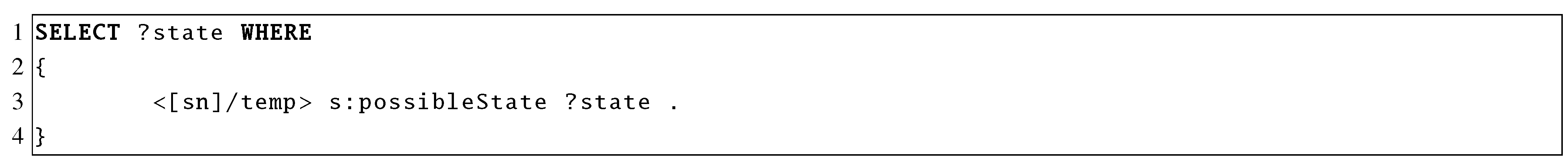
Based on this model, it is easy to formulate SPARQL queries to
retrieve all possible states of a sensor (see
Figure 9)
retrieve the state of a sensor given a sensor reading (see
Figure 10)
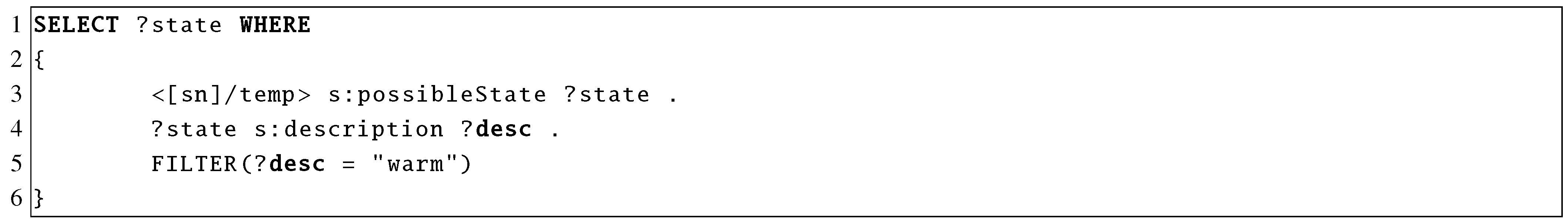
retrieve the state of a sensor for the term “warm” (see
Figure 11)
Figure 9.
Query to retrieve all possible states of the sensor.
Figure 9.
Query to retrieve all possible states of the sensor.
Table 1.
Result of query in Figure 9.
| ?state |
|---|
| warm |
| cold |
Figure 10.
Query to retrieve current state of sensor for 21 °C.
Figure 10.
Query to retrieve current state of sensor for 21 °C.
Table 2.
Result of query in Figure 10.
| ?state |
|---|
| warm |
Figure 11.
Query to retrieve state for term “warm”.
Figure 11.
Query to retrieve state for term “warm”.
Table 3.
Result of query in Figure 11.
| ?state |
|---|
| warm |
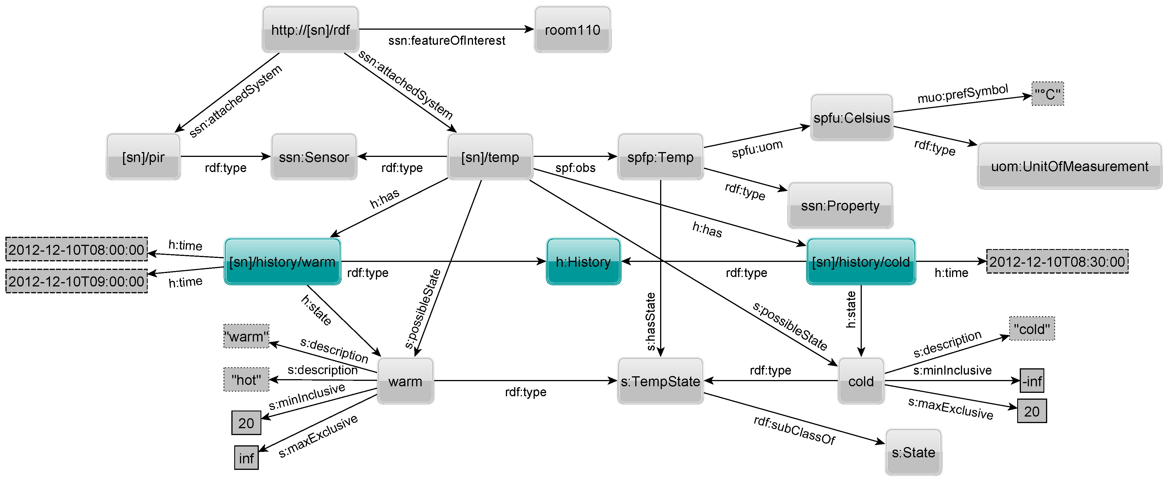
4.3. History of Sensor States
An optional history for each state can be kept for a sensor by specifying at which point in time the sensor was in a given state.
Figure 12 shows two highlighted
history nodes being linked to the temperature sensor through the property
has. Each
History element specifies for which state it holds the history via the
state property. Triples with a
time property with fully specified date and time literals (xsd:dateTime) denote when a sensor was in the associated state. The sensor is in that state from the given point in time (inclusive) until the next later timestamp (exclusive) of another state. In the example, the sensor was in warm state on the 12th of December 2012 at 8 and 9 A.M., and cold at 8:30 A.M.
Figure 12.
RDF to describe sensor state history.
Figure 12.
RDF to describe sensor state history.
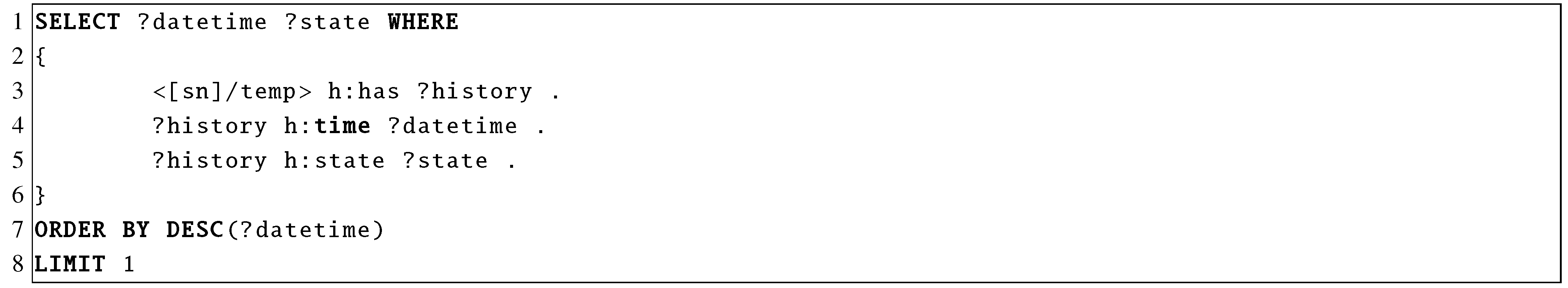
Figure 13.
Query to retrieve the latest state of the sensor.
Figure 13.
Query to retrieve the latest state of the sensor.
Table 4.
Result of query in Figure 13.
| ?datetime | ?state |
|---|
| 2012-12-10T09:00:00 | warm |
Although there exist ontologies for time such as the Time Ontology in OWL [
16], we have decided to use simple XML schema datatypes to represent instances and duration for the history and throughout the following parts of our model. This has two main reasons. First, one needs less RDF triples compared with using more complex ontologies. This also results in less complex SPARQL queries with fewer triple patterns. Second, we can use a temporal reasoner (e.g., inference based on additional RIF [
17] rules) to infer our simple-to-query data model from the durations of the more complex Time Ontology.
To store the current state of a sensor, no update operation of existing triples,
i.e., deletion and insert operation, is needed but only one new triple must be inserted.
Figure 13 shows how to query the latest state of the sensor and the associated time. After all timestamps and states have been selected (Lines 1–6), they are sorted in descending order by their time (Line 7) and finally only the first line of the resulting table is returned (Line 8) as shown in
Table 4.
4.4. The Basic Prediction Model
In the context of our work, a prediction model allows estimating the probability that a sensor reads a given state at a given point in time. There are several different approaches to predict raw sensor values (
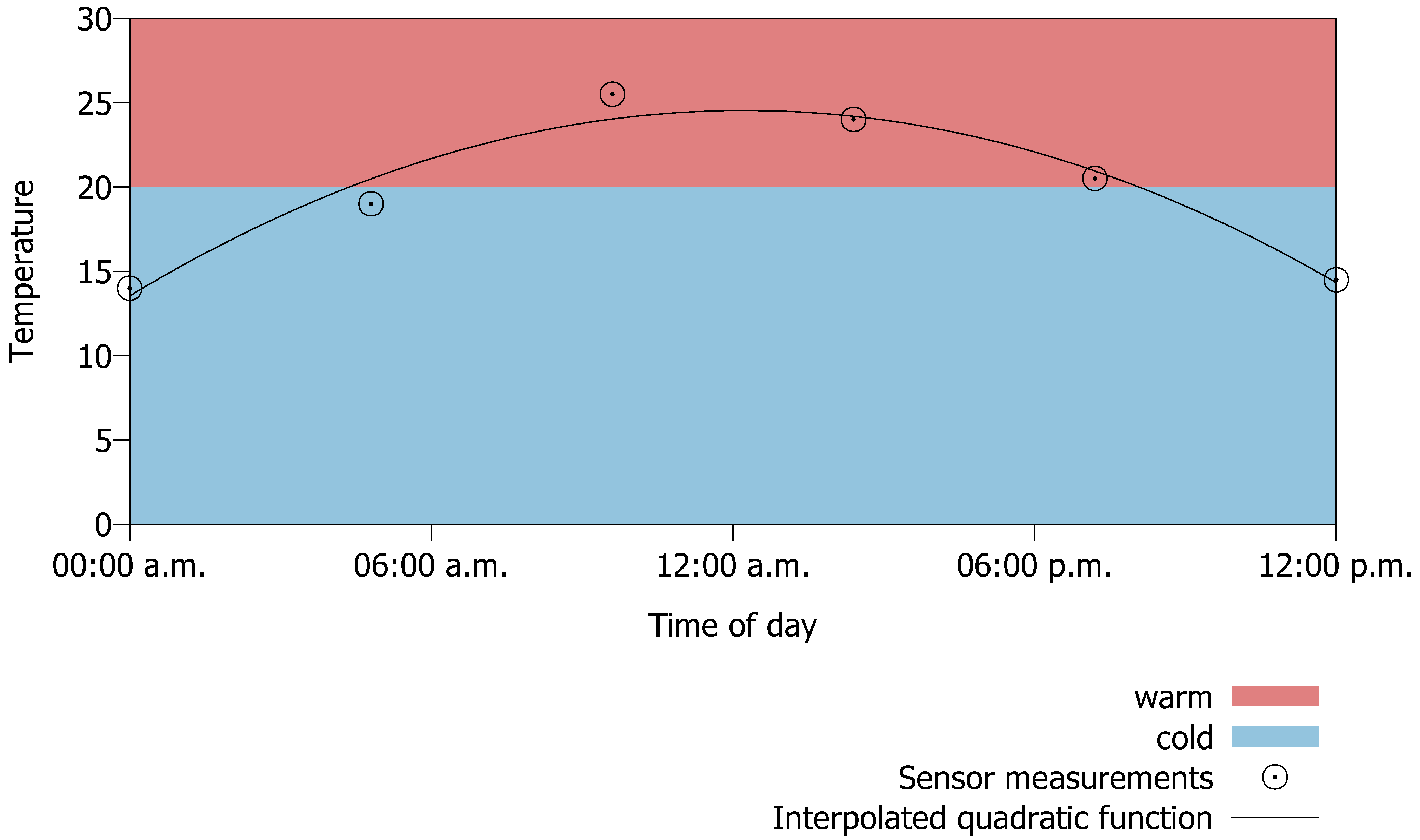
cf. Section 5). From these predictions it is easy to determine the probability for states. Consider
Figure 14, which shows six temperature sensor readings over a period of 24 hours and a sensor node interpolating a function from these readings to enable prediction of future readings. The figure shows a quadratic function that has been interpolated by selecting parameters of the function such that the sum of squared differences from the given points to the function at the same point in time is minimized. The blue and red areas show the range for the cold respectively warm state as defined in
Figure 8. One can see that most time of the day the sensor is in the warm state (approximately 65% of the time). Hence, it is 35% of the time in state cold. These percentages can be used to build the simplest prediction model called the
aggregated prediction model (APM). A sensor can only have one instance of this model.
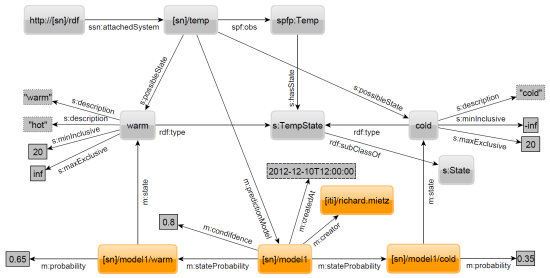
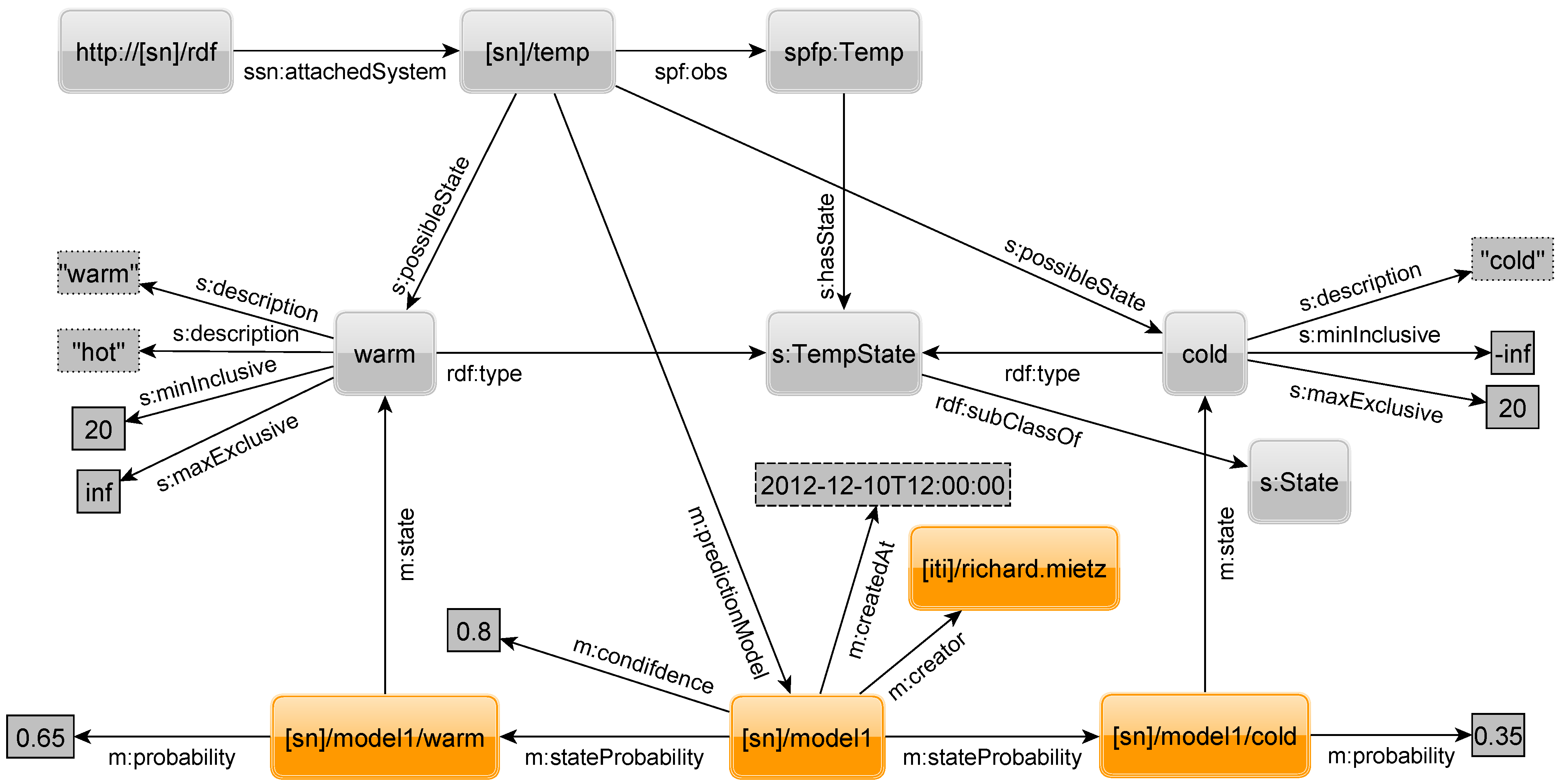
Figure 15, in which some previously introduced elements are omitted for clarity, shows how the APM is modeled using RDF. Among the highlighted elements,
model is the central resource. For each state of the sensor, we have an additional element that is connected to
model by the property
stateProbability and indicates its state by the property
state. Finally, for each state the probability is given as a float literal connected by a property
probability.
A model has additional information to show when and by whom it was created. Optionally, one can specify a confidence in the given model by a property confidence and a float literal. This can be used to filter models with a confidence above a given threshold. Furthermore, the confidence can be used to adjust the probability by multiplying it with the probability for a state. Assume the probability for the state warm is . For a model with very high confidence, e.g., , it stays nearly the same, i.e., , while for a model with low confidence such as it will decrease significantly to .
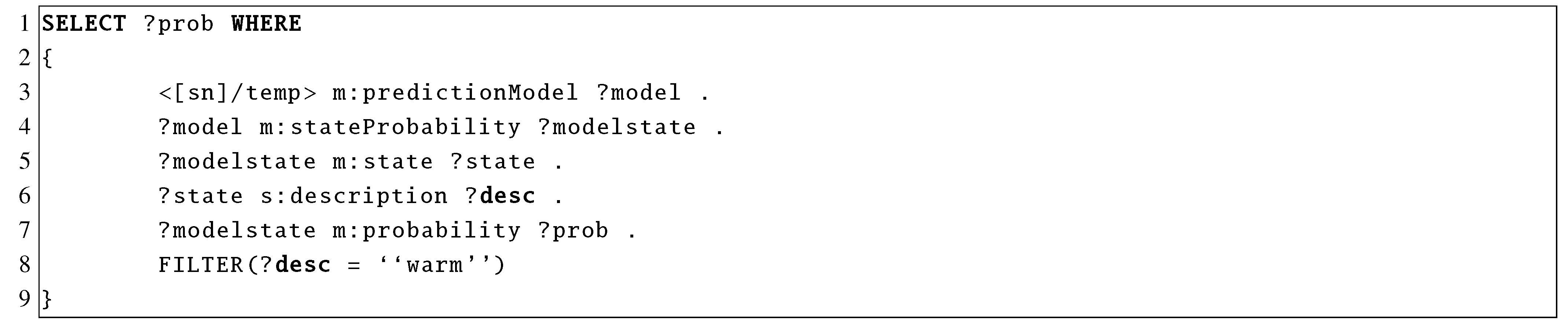
An example SPARQL query to retrieve the probability for the state “warm” is given in
Figure 16. First, the model is selected in Line 3. Lines 4–6 select the state elements of the model and the correspondent states,
i.e., both the cold and warm sub-graph. The probabilities for each state are fetched by Line 7. Finally, Line 8 removes the sub-graph for the cold state.
Figure 14.
Determine probability for states from sensor reading.
Figure 14.
Determine probability for states from sensor reading.
Figure 15.
RDF to describe an aggregated prediction model.
Figure 15.
RDF to describe an aggregated prediction model.
Figure 16.
SPARQL query to retrieve the probability for state “warm” from a given sensor.
Figure 16.
SPARQL query to retrieve the probability for state “warm” from a given sensor.
4.5. The First Refinement of the Model: Time
The APM is only effective if the state distribution does not vary substantially over time. Hence, we support other types of prediction models that take into account the time of query.
While the probabilities in an APM are always the same for a specific state of a sensor, we want them to vary over time. By adding specific triples, we can, e.g., refine the model to be only valid at specific time intervals. We will first introduce a refinement in time, afterwards show other possible refinements and finally present how one can extend the model by custom refinements.
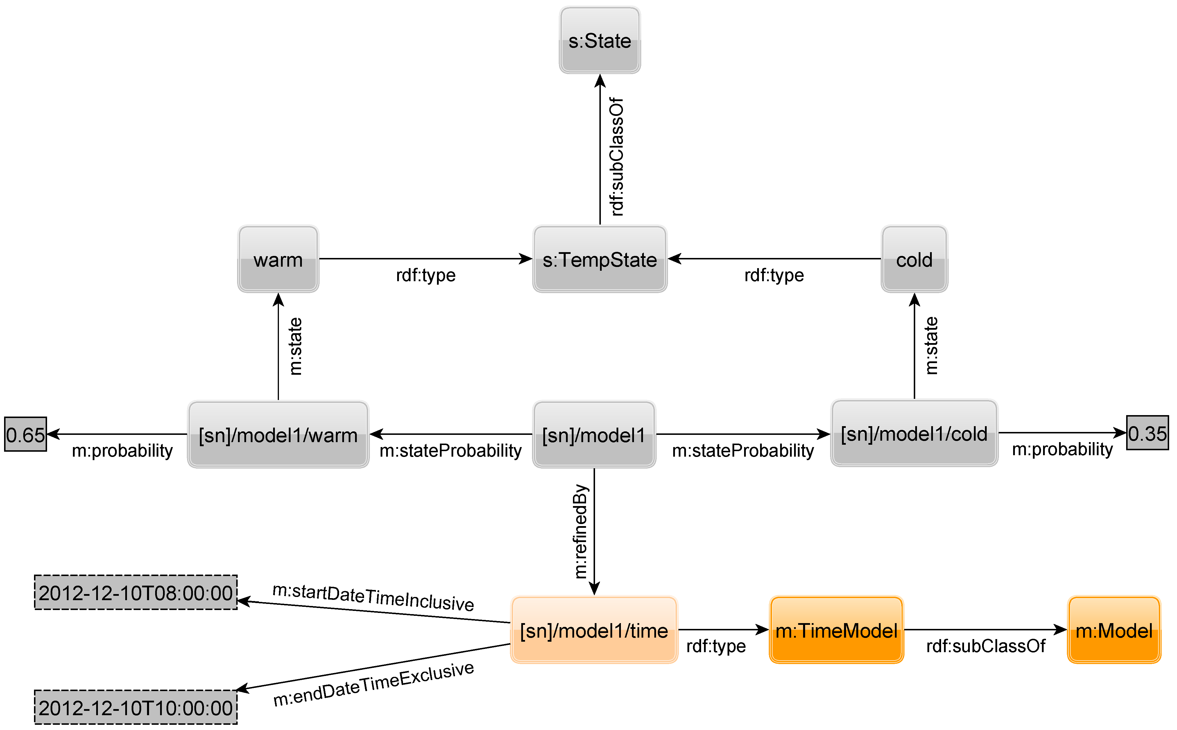
Figure 17 shows a refinement. Refinements are connected by the property
refinedBy to the appropriate APM to form a refined model, in this case a
time prediction model (TPM), which is of type
TimeModel which is in turn a subclass of
Model. In the example, the probabilities for the states are only valid between 8 A.M. (inclusive) and 10 A.M. (exclusive) on the 10th of December 2012. For all other times, we cannot estimate the probability for the states of the sensor anymore. Hence, we need to add additional prediction models to the sensor for other intervals. While there can only exist one APM for a sensor, we can have several TPMs for that sensor. However, it may be unreasonable to add models for different times of every single day. Thus, one can specify TPMs in more flexible ways.
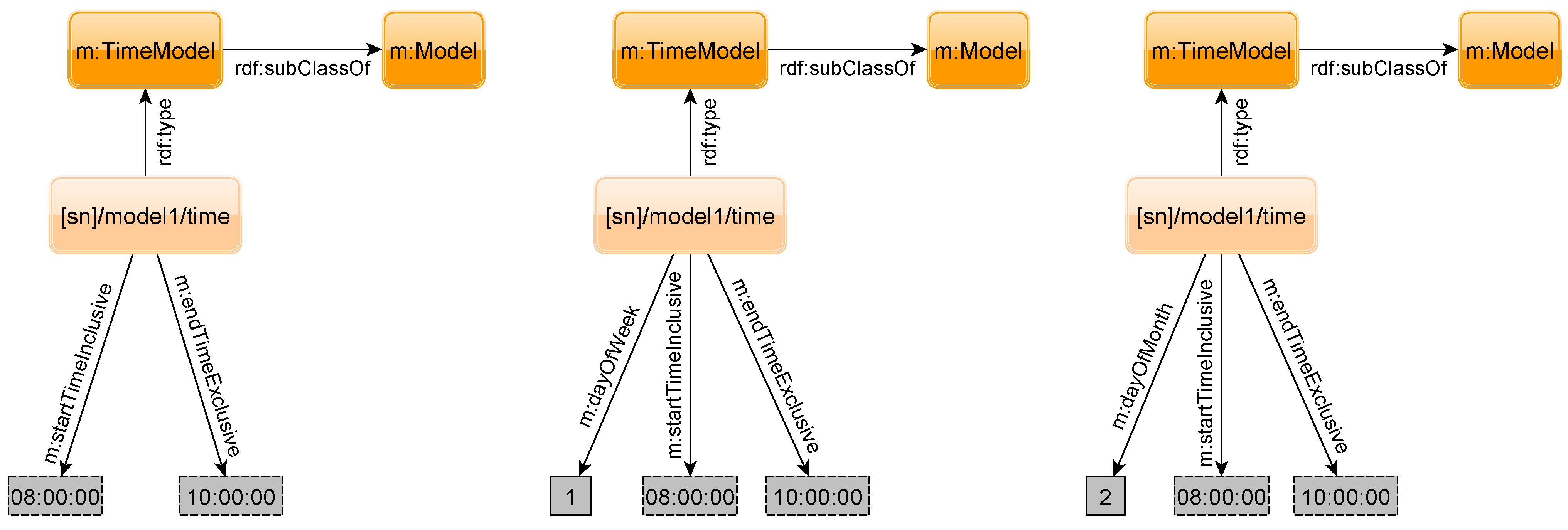
Figure 18 shows three other time refinement possibilities. The leftmost model sets the validity period of the probabilities on a daily basis. As a sensor may output different states depending on the weekday (e.g., an office might be cold on the weekend because heating is switched off), the second option is to give a period of time restricted to a specified weekday. The third possibility allows giving an interval on a specified day of the month. In the example, the validity period is every second day of the month from 8 A.M. to 10 A.M.
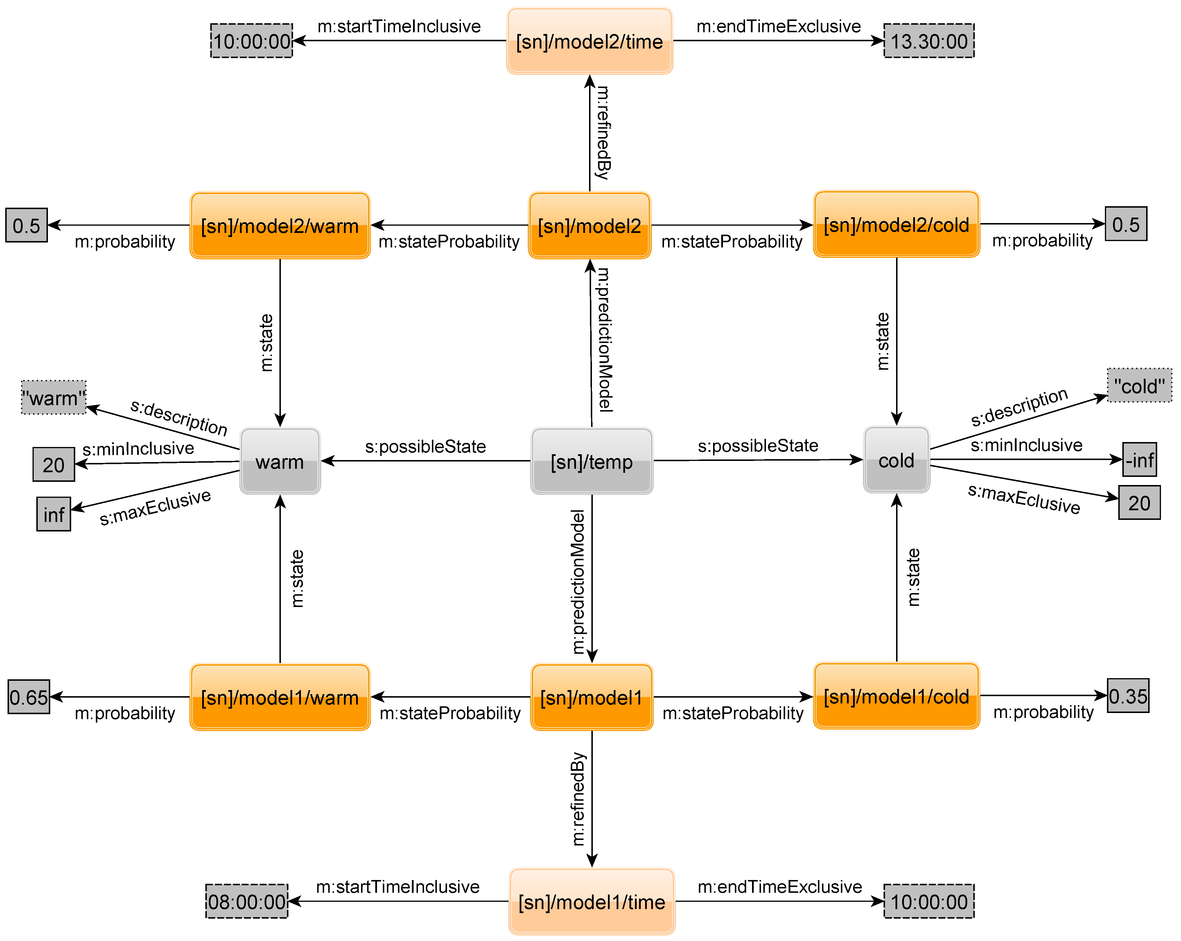
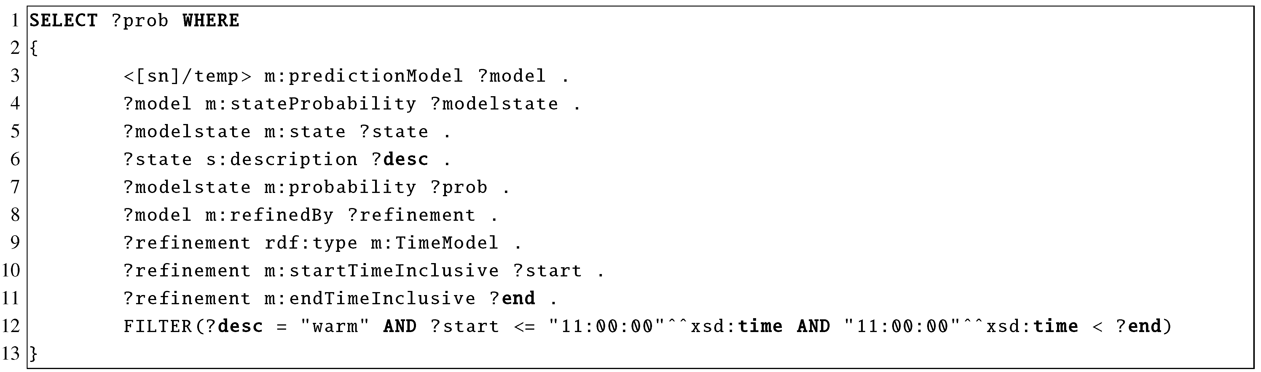
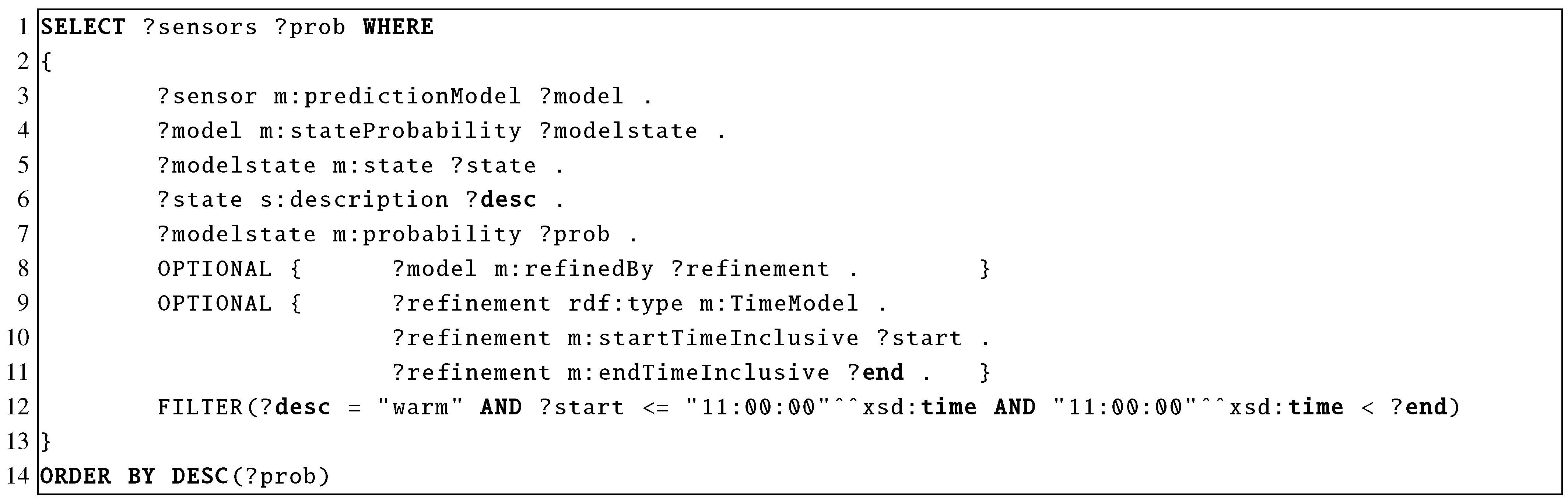
If we are searching for the probability of a sensor, we not only have the state as input, but also the time at which we want to know the probability. In
Figure 19, the sensor has two TPMs.
Figure 20 shows the query to retrieve the probability for the state
warm at 11 o’clock.
However, in order to rank sensors by probability, we must retrieve the probabilities of several sensors. To achieve this, we have to modify the first three lines of the query in
Figure 20 to the ones in
Figure 21. This retrieves all sensors and their probabilities for the desired state. Additionally, the last line was added to sort the sensors based on their probabilities to match the state. Unfortunately, this query only finds sensors that have a TPM. However, there might be sensors for which only an APM exist. Therefore, the query needs to be modified further to the one in
Figure 22. Lines 8–11 have been surrounded by the SPARQL OPTIONAL keyword. With the OPTIONAL keyword, triples can exist but they do not have to. Hence, the TPM is selected if it exists, but if not, the APM will still be selected. In such a way, the probabilities of sensors with different kinds of models can be retrieved with a single query.
Figure 17.
RDF to describe a time-dependent prediction model.
Figure 17.
RDF to describe a time-dependent prediction model.
Figure 18.
Variants of the time-dependent prediction model.
Figure 18.
Variants of the time-dependent prediction model.
Figure 19.
Sensor with two TPMs.
Figure 19.
Sensor with two TPMs.
Figure 20.
SPARQL query to retrieve the probability for state “warm” at 11 o’clock from a given sensor.
Figure 20.
SPARQL query to retrieve the probability for state “warm” at 11 o’clock from a given sensor.
Figure 21.
Needed modification for SPARQL query in
Figure 20.
Figure 21.
Needed modification for SPARQL query in
Figure 20.
Figure 22.
SPARQL Query to select all sensors having a TPM or APM.
Figure 22.
SPARQL Query to select all sensors having a TPM or APM.
4.6. Further Refinements: Place and Correlation
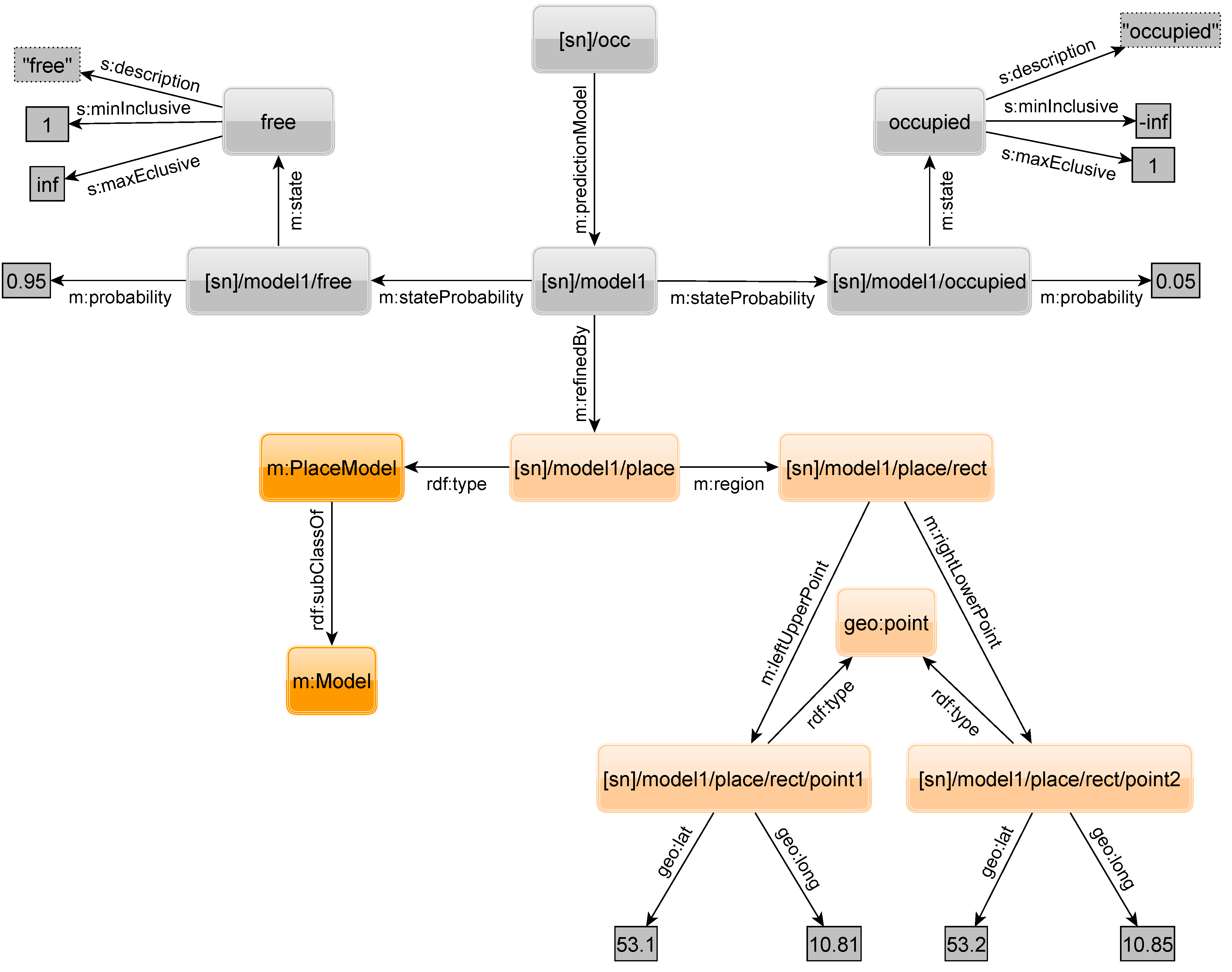
As already mentioned, time is not the only physical property that influences probabilities of sensor states. Let us assume there are sensors attached to mobile entities where the probability for a state depends on an entity’s location. Assume, e.g., a sensor measuring the occupancy of a taxi. When the taxi brings people to a concert, it will be empty at the concert hall after delivering the passengers there. The graph in
Figure 23 shows the states
free and
occupied (the probabilities for these states), but also a spatial refinement resulting in a place prediction model
PPM. The place or more exactly the area is given by two geographic points (latitude and longitude) that span a rectangle. An arbitrary number of rectangles can be appended to narrow down other shapes or add other regions. With such a model, one could state that somewhere else in the city the taxi is much more likely to be occupied. However, the probability at a concert hall for a free taxi might also depend on the time. Imagine the concert is over and all the attendees want to get a taxi home. Fortunately, our model allows combining refinements of different types, e.g., a TPM and PPM. A query that can handle the PPM needs additional OPTIONAL triple patterns to select the PPM related triple. Also, the location to search at must be given in the query to select the geographically correct PPM.
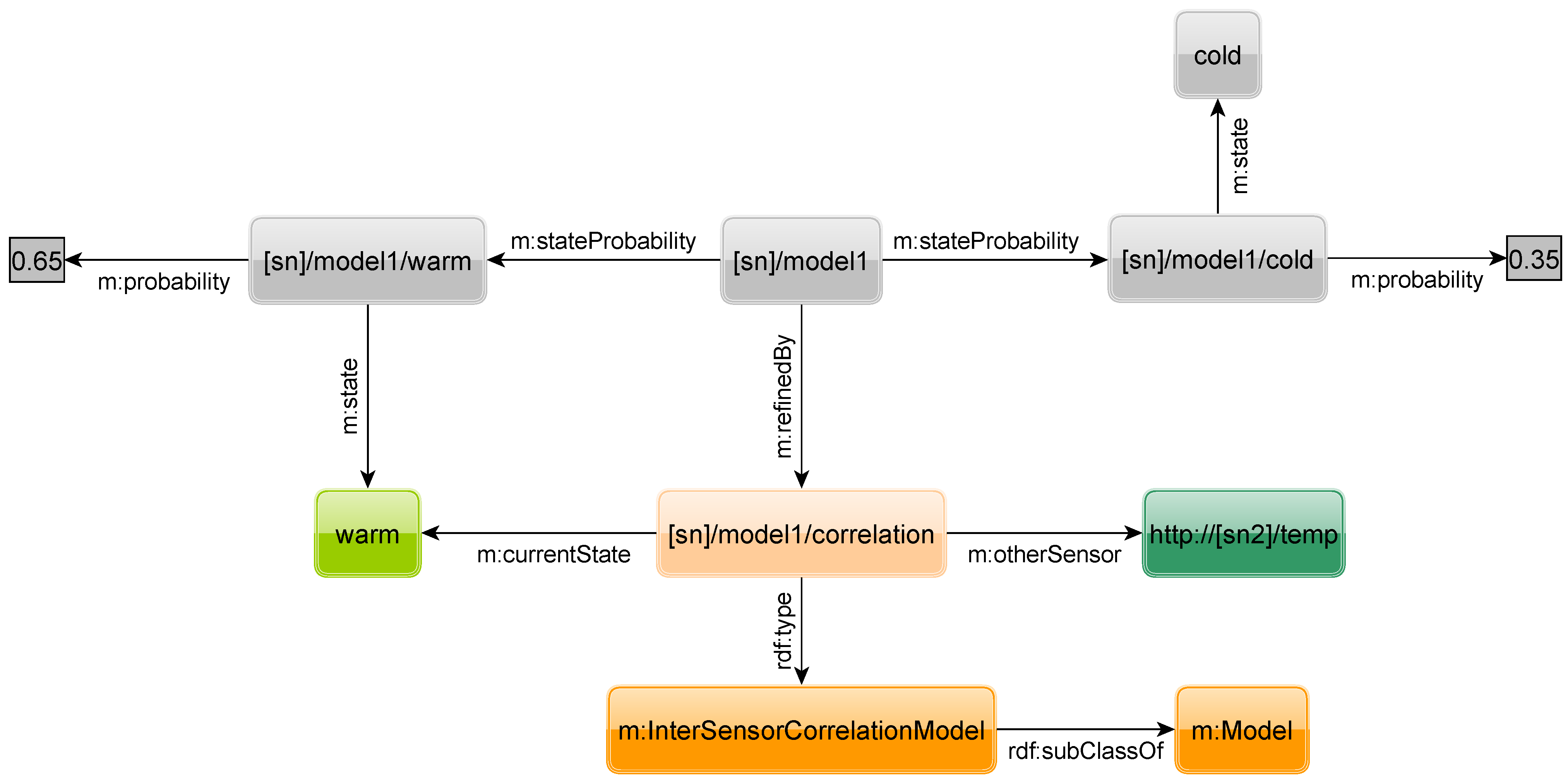
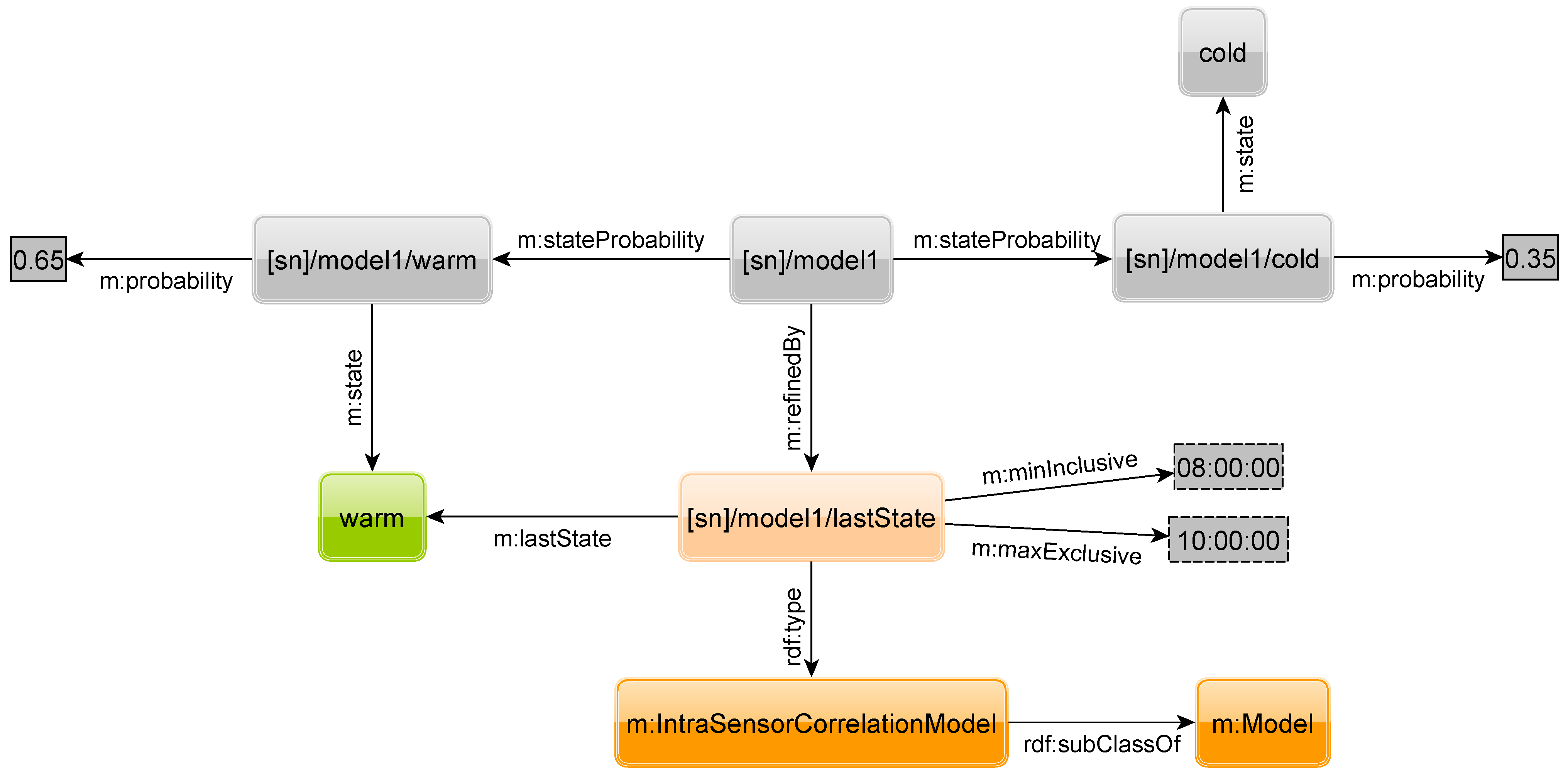
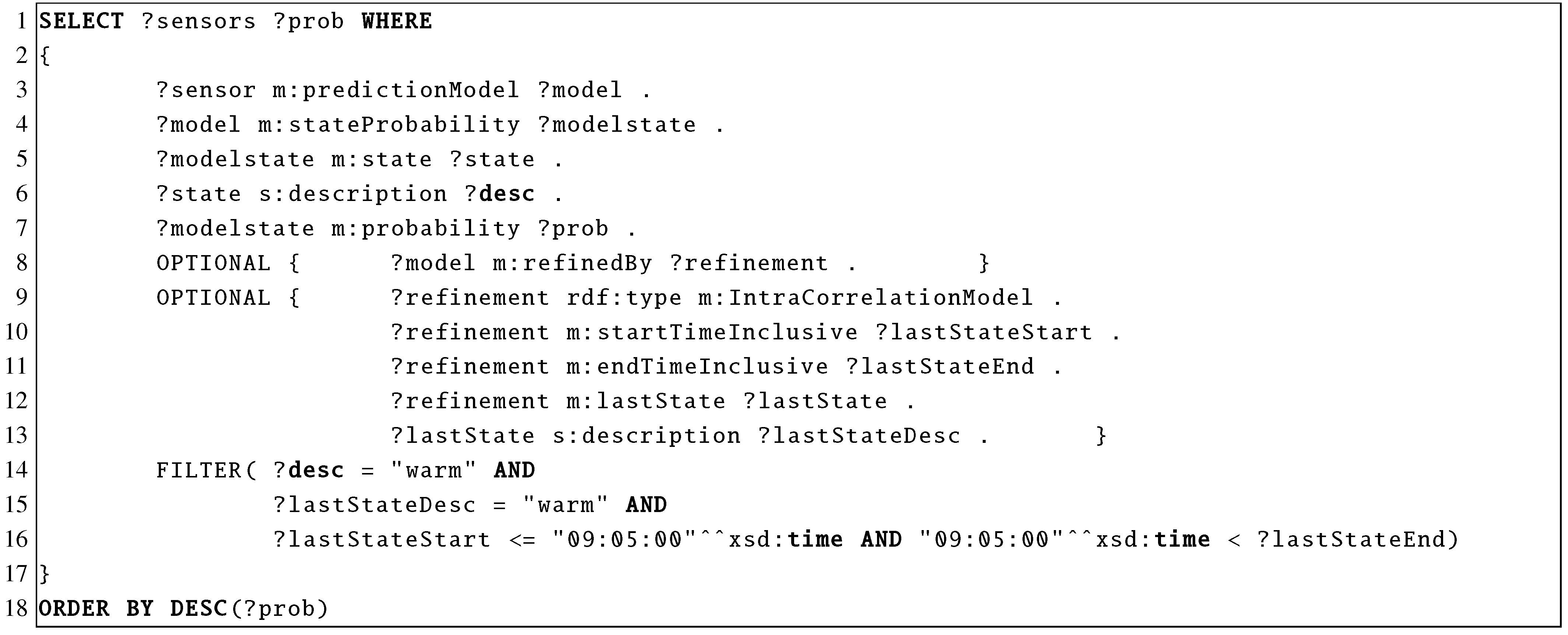
Figure 24 and
Figure 25 show two other possible refinements. The first models the intra-sensor correlation of sensor readings obtained from the same sensor, e.g., between the current and a past sensor reading, while the second models the inter-sensor correlation of values obtained from different sensors,
i.e., between the reading of sensors of same type on different sensor nodes. A query for the intra-sensor correlation model is given in
Figure 26. With the OPTIONAL keywords in lines 9–13 we select the triples of the model. Line 14 states that we are searching for state
warm. Lines 15 and 16 specify that we know that at 9:05 the state of the sensor was also
warm.
In general, one sensor can have an arbitrary number of models with refinements. For each refinement, the query must be extended with the proper OPTIONAL patterns and other needed input such as time or place to select the correct model.
Figure 23.
Sensor with Place Refinement.
Figure 23.
Sensor with Place Refinement.
4.7. Defining Custom Refinements
We presented different types of time, place, and correlation refinements for the base prediction model. However, there are many other conditions where the probability of a sensor (or more precisely of an entity) can depend on. For example, environmental sensors measuring humidity, temperature, or wind can depend on the weather forecast.
The proposed model is easy to extend and allows arbitrary other refinements. It is only required to formulate new model as a set of triples and add it to the base model by a property refinedBy. To use the new model, queries need to be adjusted by adding appropriate OPTIONAL triple patterns to the presented queries.
Figure 24.
Intra-sensor correlation.
Figure 24.
Intra-sensor correlation.
Figure 25.
Inter-sensor correlation.
Figure 25.
Inter-sensor correlation.
Figure 26.
SPARQL Query for the intra-sensor correlation model.
Figure 26.
SPARQL Query for the intra-sensor correlation model.
4.8. Analysis of the Complete Model
Prediction Models and their assigned state probabilities will change with much lower frequency than sensor states. However, from time to time updates to the models are needed. This includes updating the state probabilities, insertion of new models, deletion of outdated models, or updating of existing models. DELETE, UPDATE and INSERT operations are usually supported by SPARQL endpoints by means of SPARQL 1.1 Update [
18].
Table 5 gives a short summary on how many triples are needed for each presented part to convey an idea of how many triples are generated by a single sensor to publish its states and prediction models. As one can see, the static number of triples for each concept is rather small. The number of needed triples in some concepts of the model is depending on a variable. But even these parts are linearly dependent, resulting in an overall small number of triples for the final model. This is in line with the scalability requirements of the IoT connecting billions of sensors
Table 5.
Summary of needed triples for the presented concepts.
Table 5.
Summary of needed triples for the presented concepts.
| Concept | Dependent Variable | # of Triples |
|---|
| A global defined state | # of descriptive terms | |
| States for a sensor | # of sensor states | |
| History for a state | # of point in times the sensor was in the history’s state | |
| APM | | |
| TPM | # of validity periods | |
| PPM | # of geographical regions | |
| intra-CPM | – | |
| inter-CPM | – | |
The complexity of SPARQL queries grows with the complexity of the corresponding models,
i.e., the number of triple patterns in a SPARQL query grows linearly with the number of triples needed for a prediction model. However, this is of course true for the whole semantic web. If data are too diverse, one needs complex queries to find relevant data. In the scope of this paper, we do not explicitly address this concern because it is a general problem in this domain. For future work, we envision that RIF rules [
17] could ease this process. A simple SPARQL query without OPTIONAL patterns for each prediction model would initiate a process of selecting the appropriate probability from the different types of prediction models at query time.
5. Related Work
Several systems [
19,
20,
21,
22,
23,
24,
25] have been proposed that use prediction models to efficiently answer queries for values of sensors in wireless sensor networks. While some approaches generate prediction models at the base station (BS), others do this at the sensor node itself. Both approaches have advantages and disadvantages. The generation of a model requires a certain amount of sensor data. Thus, if generated at a BS, these data have to be collected first,
i.e., sent through the network and hence consume resources in terms of bandwidth and energy. However, this allows exploiting correlations and powerful models. In contrast, model generation on sensor nodes enables faster reaction to changes and needs fewer resources as only parameters of the model need to be sent to the BS.
In [
22] every sensor node sends an estimation of its sensor values in terms of an interval to a BS. Queries include an error margin. If the margin is smaller than the stored interval for that node, the BS can answer directly. Otherwise, the sensor node is contacted for its current reading. The sensor node checks periodically if the interval stored at the BS is still a good approximation of its current values and updates it if necessary.
BBQ [
19] constructs prediction models for sensor nodes at the BS based on historical data. Similar to [
22], the queries include an error margin. The BS checks if the prediction’s accuracy is sufficient. If not, the sensor node is queried. Because the nodes themselves are neither sending values nor do they check the quality of the models, outliers are not detected. While BBQ uses a pull-based approach, KEN [
20] uses a push-based one. As in BBQ, the BS uses prediction models to answer queries. But the models are also kept at the sensor nodes at the same time. A sensor node compares its predictions of the model with the readings of the sensor. If they do not match, corrections are sent to the BS. Thus, outliers can be detected.
Although every sensor node builds a prediction model in PAQ [
23], not all are sent to the BS. Instead, nodes with similar models cluster together. The cluster head is then sending only one model to the BS that is representative for all nodes in the cluster. Like BBQ, the nodes evaluate their models from time to time and update them if necessary. An improvement of PAQ is described in [
24]. First, another type of model is used, and second, the nodes send their models to the BS so that the BS is building the clusters. Hence, also nodes far from each other can end up in the same cluster.
Also PRESTO [
21] shares many aspects with PAQ, KEN, and BBQ. The main difference is the use of a more sophisticated type of prediction model.
In ASAP [
25], nodes are initially clustered by similar sensor values and spatial proximity. Afterwards, the cluster head collects sensor readings of all cluster members and divides the cluster in sub-clusters by means of correlations between their readings. In each sub-cluster, a node is selected to report its readings periodically to the BS. The values of non-sending nodes are estimated at the BS with the help of correlation-based prediction models. The models are also updated periodically.
All presented systems are designed for efficient querying of continuous sensor readings of specific sensor nodes with the help of prediction models and error margins. Searching sensor nodes with a certain raw reading or discrete state is not supported. While the presented systems use time-series and correlation-based models, we presented a way to generally describe and use prediction models for efficient search.
6. Conclusion and Future Work
We are currently witnessing the emergence of Internet of Things, where smart devices perceive and publish the state of the real world online. Global search for sensors currently reading a given state will be a fundamental service in the Internet of Things that requires novel concepts as the state of sensors changes very rapidly. To this end, the use of prediction models to estimate the current state of a sensor without actually reading its output is a promising strategy. In this paper we propose the use of Semantic Web technologies to implement this concept by encoding prediction models as RDF graphs and by formulating SPARQL queries to evaluate the prediction models to obtain a ranked list of sensors.
The effectiveness of using prediction models to reduce resource consumption on sensor nodes and to speed up the search process strongly depends on the quality of the prediction models. While creating good predictions for sensor states is out of the scope of this paper, we will investigate this in future work. Also, as different sensors may require different search strategies, our future work will focus on identifying a set of different approaches that cover the most common types of sensors. Based on that, we will investigate adaptation algorithms to automatically select the most appropriate search strategies. Our work will be guided by the analysis of different sensor data sets.
For our considered scenarios, we currently model only rudimentary spatial and temporal constraints and define therefore a simple but easy-to-use model. However, if the requirements of the considered scenarios increase and lead to more complex spatial and temporal constraints, we will extend our model for integrating spatial-temporal ontologies and using spatial-temporal extensions of SPARQL (e.g., GeoSPARQL [
26], SOWL [
27], SPARQL-ST [
28] and the continuum model [
29]).


