Instability Index Derived from a Landslide Inventory for Watershed Stability Assessment and Mapping


Abstract
:1. Introduction
2. Materials and Methods
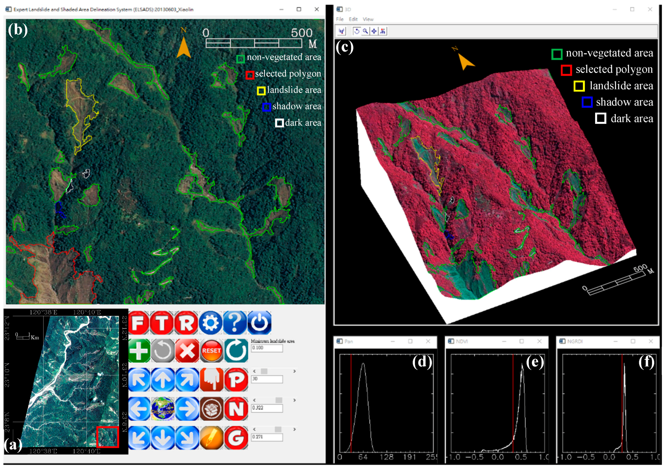
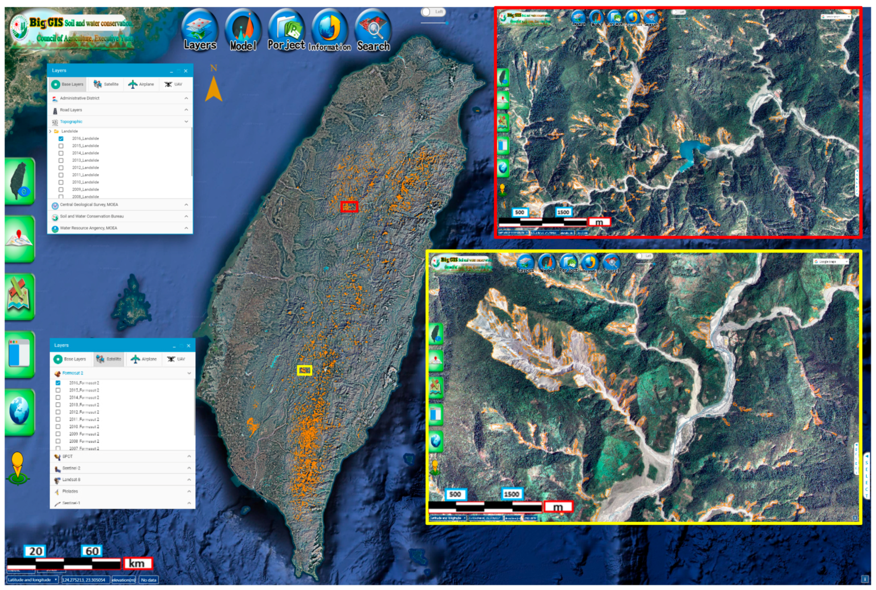
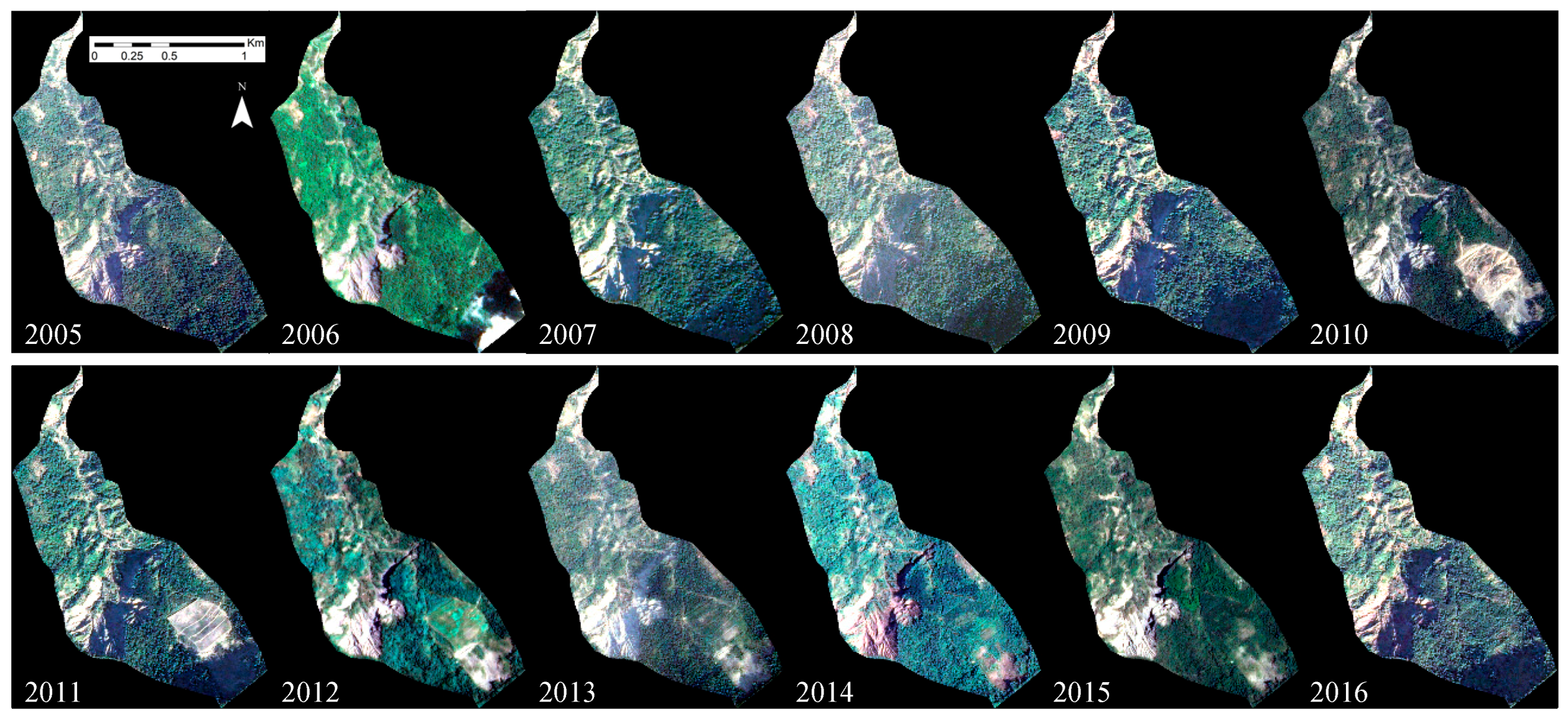
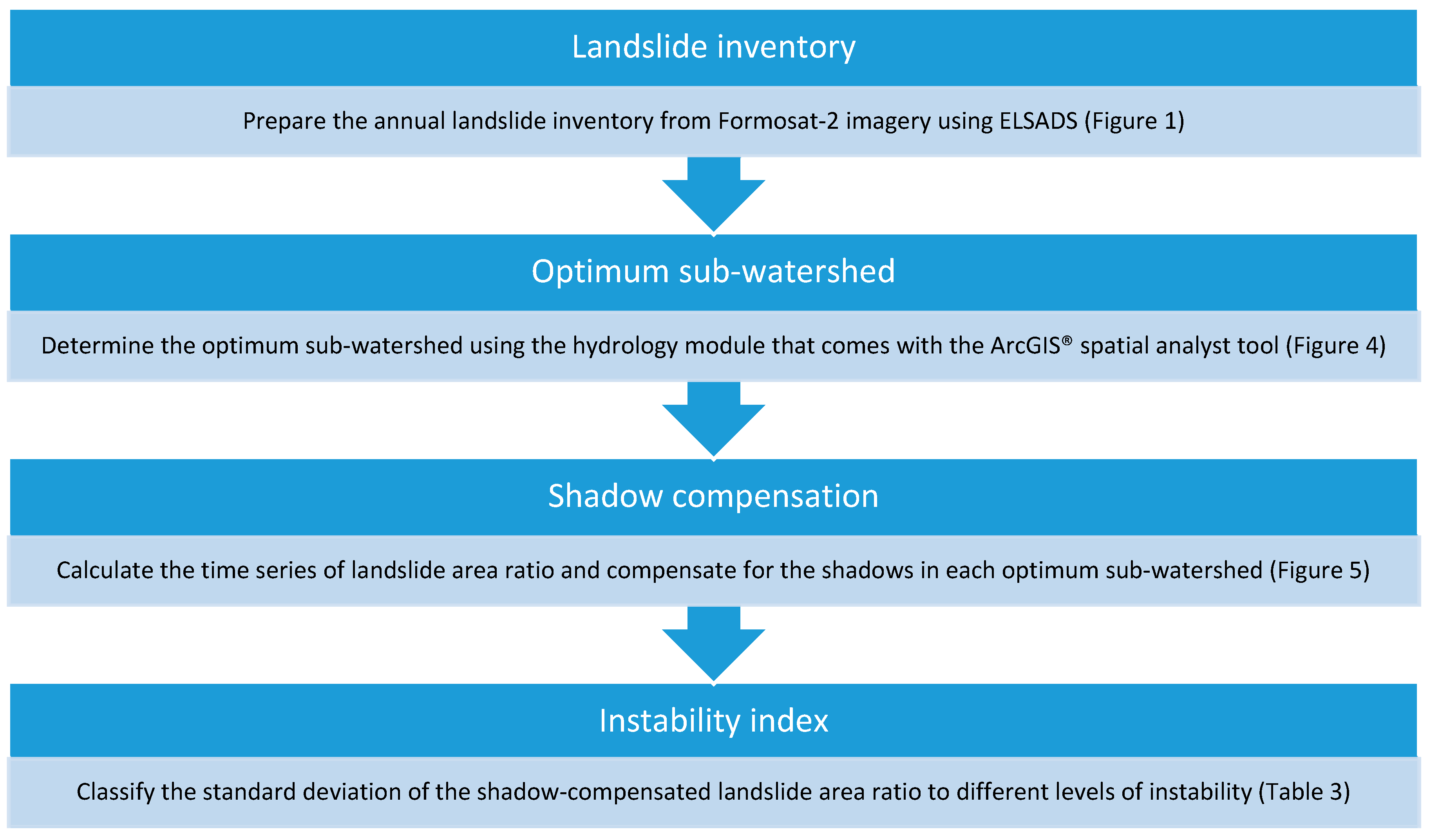
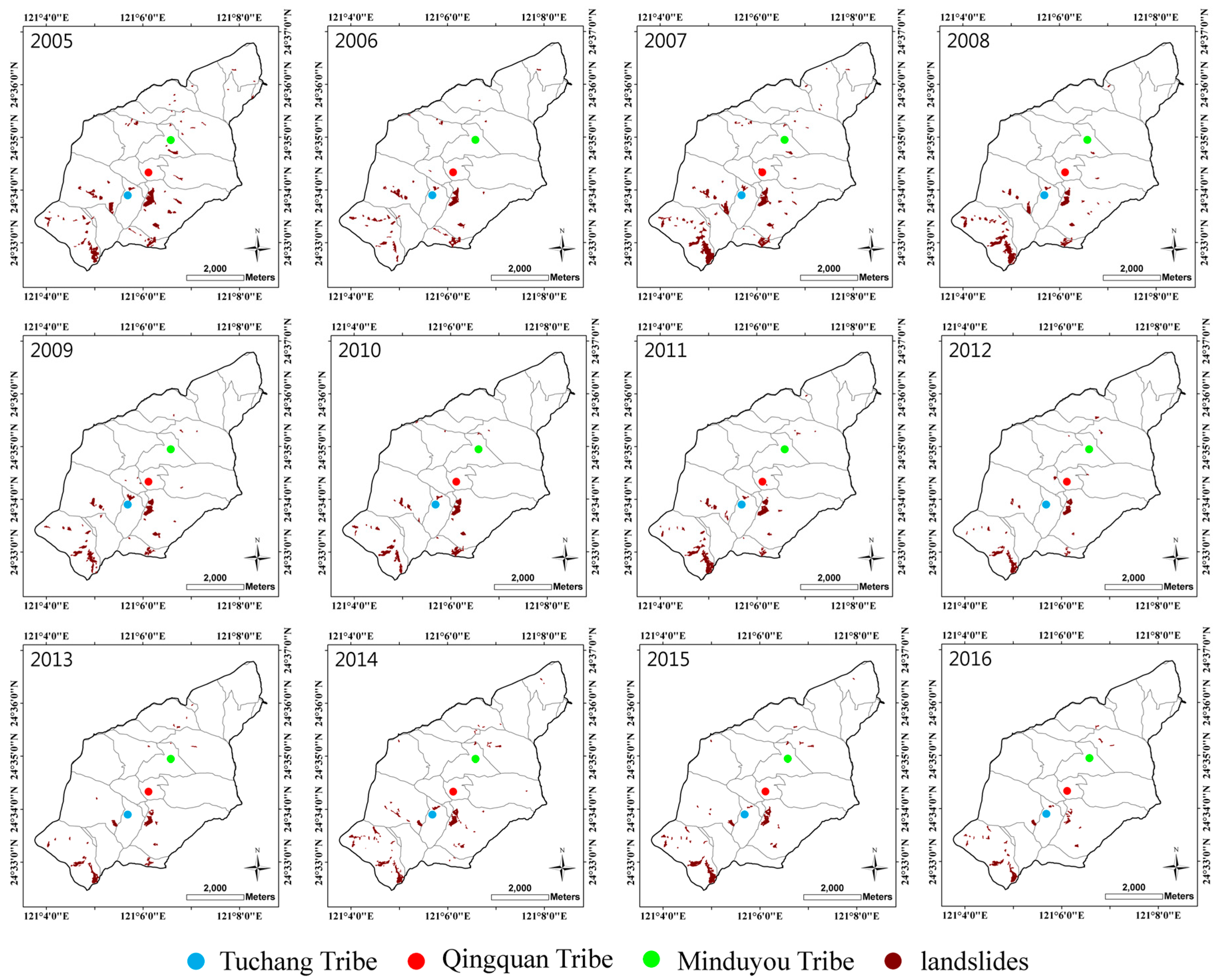
2.1. Landslide Inventory
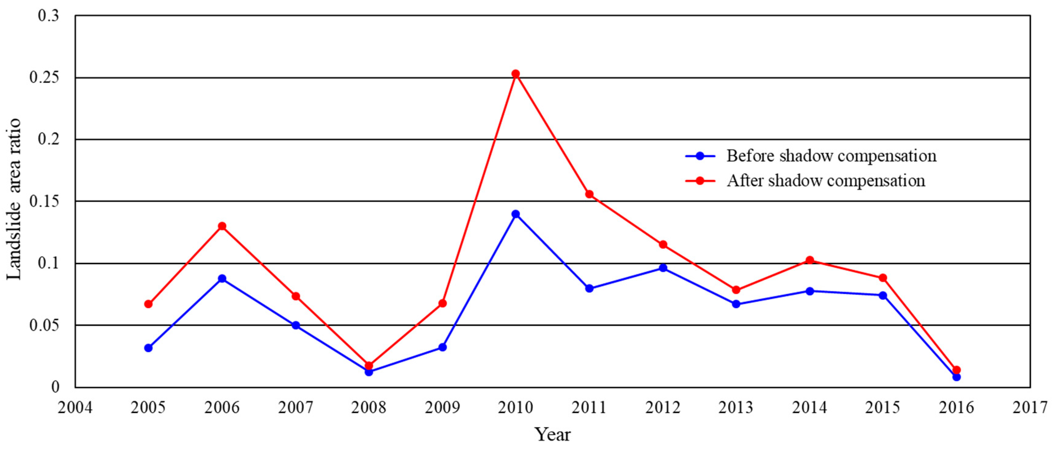
2.2. Quantitative Assessment
2.2.1. Governance of Watershed Management and Flood Mitigation Units
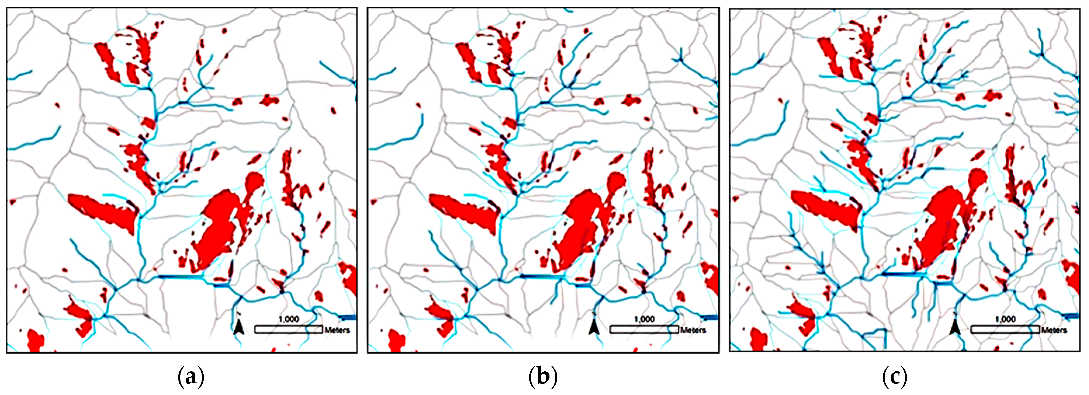
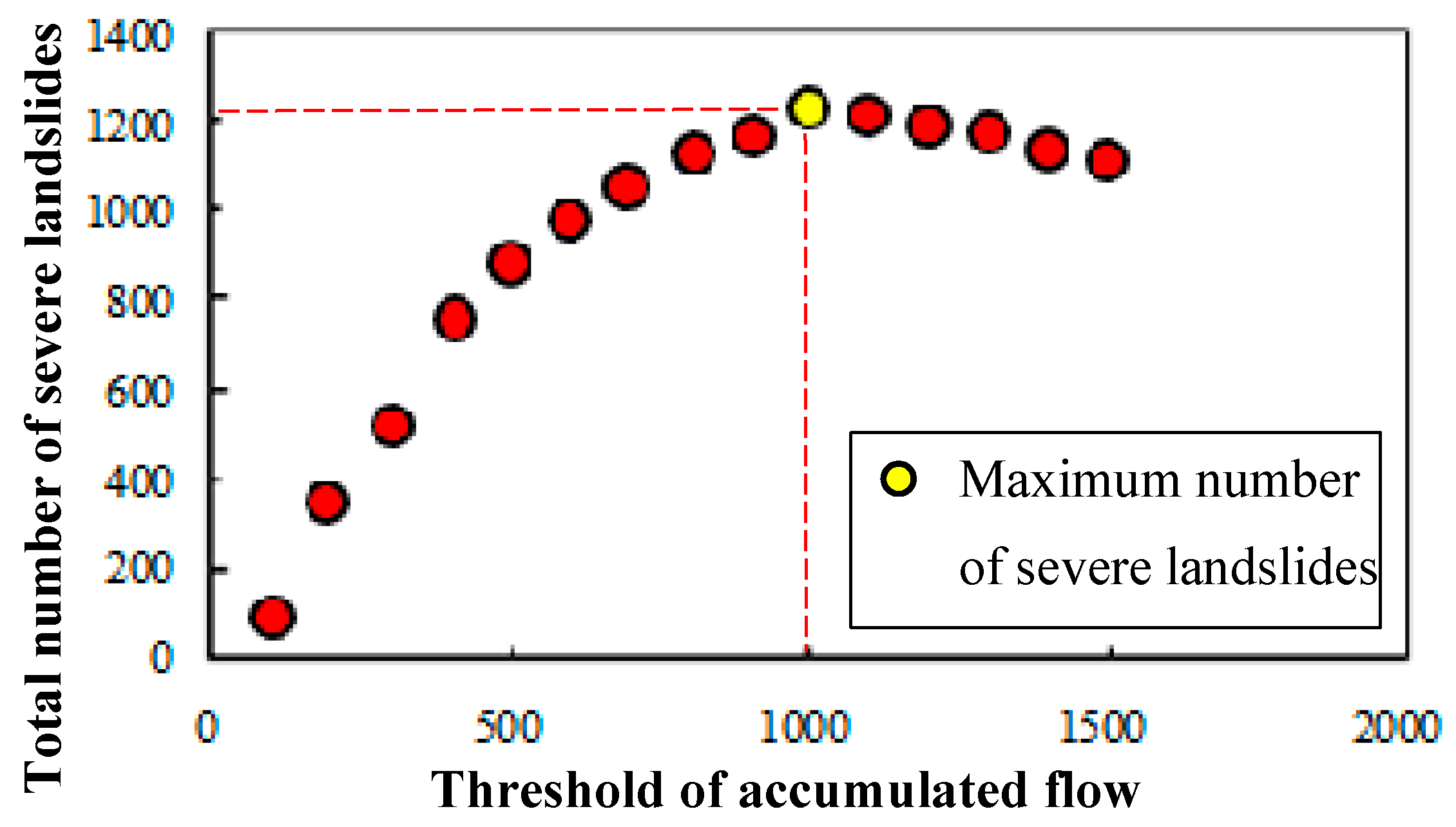
2.2.2. Optimum Sub-Watershed
2.2.3. Instability Index
3. Results
4. Discussion
5. Conclusions
Author Contributions
Funding
Acknowledgments
Conflicts of Interest
References
- Moore, J.W.; Beakes, M.P.; Nesbitt, H.K.; Yeakel, J.D.; Patterson, D.A.; Thompson, L.A.; Phillis, C.C.; Braun, D.C.; Favaro, C.; Scott, D. Emergent stability in a large, free-flowing watershed. Ecology 2015, 96, 340–347. [Google Scholar] [CrossRef] [PubMed]
- Pimentel, D. Soil erosion and the threat to food security and the environment. Ecosyst. Health 2000, 6, 221–226. [Google Scholar] [CrossRef]
- Chou, C.; Chen, C.-A.; Tan, P.-H.; Chen, K.T. Mechanisms for global warming impacts on precipitation frequency and intensity. J. Clim. 2012, 25, 3291–3306. [Google Scholar] [CrossRef]
- Mirza, M.M.Q. Global warming and changes in the probability of occurrence of floods in bangladesh and implications. Glob. Environ. Chang. 2002, 12, 127–138. [Google Scholar] [CrossRef]
- Alfieri, L.; Burek, P.; Feyen, L.; Forzieri, G. Global warming increases the frequency of river floods in europe. Hydrol. Earth Syst. Sci. 2015, 19, 2247–2260. [Google Scholar] [CrossRef]
- Koukis, G.; Ziourkas, C. Slope instability phenomena in greece: A statistical analysis. Bull. Int. Assoc. Eng. Geol. 1991, 43, 47–60. [Google Scholar] [CrossRef]
- Süzen, M.L.; Kaya, B.Ş. Evaluation of environmental parameters in logistic regression models for landslide susceptibility mapping. Int. J. Digit. Earth 2011, 5, 338–355. [Google Scholar] [CrossRef]
- Liu, C.-C.; Luo, W.; Chen, M.-C.; Lin, Y.-T.; Wen, H.-L. A new region-based preparatory factor for landslide susceptibility models: The total flux. Landslides 2016, 13, 1049–1056. [Google Scholar] [CrossRef]
- Cosh, M.H.; Jackson, T.J.; Bindlish, R.; Prueger, J.H. Watershed scale temporal and spatial stability of soil moisture and its role in validating satellite estimates. Remote Sens. Environ. 2004, 92, 427–435. [Google Scholar] [CrossRef]
- Hu, W.; Shao, M.; Wang, Q.; Reichardt, K. Time stability of soil water storage measured by neutron probe and the effects of calibration procedures in a small watershed. Catena 2009, 79, 72–82. [Google Scholar] [CrossRef]
- Rowbotham, D.N.; Dudycha, D. Gis modelling of slope stability in phewa tal watershed, Nepal. Geomorphology 1998, 26, 151–170. [Google Scholar] [CrossRef]
- Liu, C.-C.; Ko, M.-H.; Lin, Y.-T.; Huang, C.-S.; Chen, C.-Y. Nowcasting of landslides. SPIE Newsroom, 27 May 2015. [Google Scholar]
- Dadson, S.J.; Hovius, N.; Chen, H.; Dade, W.B.; Hsieh, M.-L.; Willett, S.D.; Hu, J.-C.; Horng, M.-J.; Chen, M.-C.; Stark, C.P.; et al. Links between erosion, runoff variability and seismicity in the taiwan orogen. Nature 2003, 426, 648–651. [Google Scholar] [CrossRef] [PubMed]
- Dilley, M.; Chen, R.S.; Deichmann, U.; Lerner-Lam, A.L.; Arnold, M.; Agwe, J.; Buys, P.; Kjekstad, O.; Lyon, B.; Yetman, G. Natural Disaster Hotspots: A Global Risk Analysis; World Bank Publications: Washington, DC, USA, 2005; p. 29. [Google Scholar]
- Liu, C.-C. Preparing a landslide and shadow inventory map from high-spatial-resolution imagery facilitated by an expert system. J. Appl. Remote Sens. 2015, 9, 096080. [Google Scholar] [CrossRef]
- Di Paola, G.; Alberico, I.; Aucelli, P.; Matano, F.; Rizzo, A.; Vilardo, G. Coastal subsidence detected by synthetic aperture radar interferometry and its effects coupled with future sea-level rise: The case of the sele plain (Southern Italy). J. Flood Risk Manag. 2018, 11, 191–206. [Google Scholar] [CrossRef]
- Stamatopoulos, C.; Petridis, P.; Parcharidis, I.; Foumelis, M. A method predicting pumping-induced ground settlement using back-analysis and its application in the karla region of greece. Nat. Hazards 2018, 92, 1733–1762. [Google Scholar] [CrossRef]
- Hervás, J. Landslide inventory. In Encyclopedia of Natural Hazards; Bobrowsky, P.T., Ed.; Springer: Dordrecht, The Netherlands, 2013; pp. 610–611. [Google Scholar]
- Spiker, E.C.; Gori, P.; Survey, G. National Landslide Hazards Mitigation Strategy, a Framework for Loss Reduction; U.S. Geological Survey: Reston, VA, USA, 2003.
- Lin, E.-J.; Liu, C.-C.; Chang, C.-H.; Cheng, I.-F.; Ko, M.-H. Using the formosat-2 high spatial and temporal resolution multispectral image for analysis and interpretation landslide disasters in taiwan. J. Photogramm. Remote Sens. 2013, 17, 31–51. [Google Scholar]
- Liu, C.-C. Processing of formosat-2 daily revisit imagery for site surveillance. IEEE Trans. Geosci. Remote Sens. 2006, 44, 3206–3214. [Google Scholar] [CrossRef]
- Liu, C.-C.; Liu, J.-G.; Lin, C.-W.; Wu, A.-M.; Liu, S.-H.; Shieh, C.-L. Image processing of formosat-2 data for monitoring south asia tsunami. Int. J. Remote Sens. 2007, 28, 3093–3111. [Google Scholar] [CrossRef]
- Liu, C.-C.; Chen, P.-L. Automatic extraction of ground control regions and orthorectification of formosat-2 imagery. Opt. Express 2009, 17, 7970–7984. [Google Scholar] [CrossRef]
- Liu, C.-C.; Shieh, C.-L.; Wu, C.-A.; Shieh, M.-L. Change detection of gravel mining on riverbeds from the multi-temporal and high-spatial-resolution formosat-2 imagery. River Res. Appl. 2009, 25, 1136–1152. [Google Scholar] [CrossRef]
- Chang, C.-H.; Liu, C.-C.; Wen, C.-G.; Cheng, I.-F.; Tam, C.-K.; Huang, C.-S. Monitoring reservoir water quality with formosat-2 high spatiotemporal imagery. J. Environ. Monit. 2009, 11, 1982–1992. [Google Scholar] [CrossRef] [PubMed]
- Liu, C.-C.; Kamei, A.; Hsu, K.H.; Tsuchida, S.; Huang, H.M.; Kato, S.; Nakamura, R.; Wu, A.M. Vicarious calibration of the formosat-2 remote sensing instrument. IEEE Trans. Geosci. Remote Sens. 2010, 48, 2162–2169. [Google Scholar]
- Fourniadis, I.G.; Liu, J.G.; Mason, P.J. Regional assessment of landslide impact in the three gorges area, china, using aster data: Wushan-zigui. Landslides 2007, 4, 267–278. [Google Scholar] [CrossRef]
- Metternicht, G.; Hurni, L.; Gogu, R. Remote sensing of landslides: An analysis of the potential contribution to geo-spatial systems for hazard assessment in mountainous environments. Remote Sens. Environ. 2005, 98, 284–303. [Google Scholar] [CrossRef]
- Xu, M.; Cao, C.; Zhang, H.; Guo, J.; Nakane, K.; He, Q.; Guo, J.; Chang, C.; Bao, Y.; Gao, M.; et al. Change detection of an earthquake-induced barrier lake based on remote sensing image classification. Int. J. Remote Sens. 2010, 31, 3521–3534. [Google Scholar] [CrossRef]
- Nichol, J.; Wong, M.S. Satellite remote sensing for detailed landslide inventories using change detection and image fusion. Int. J. Remote Sens. 2005, 26, 1913–1926. [Google Scholar] [CrossRef]
- Nichol, J.; Wong, M.S. Detection and interpretation of landslides using satellite images. Land Degrad. Dev. 2005, 16, 243–255. [Google Scholar] [CrossRef]
- Dymond, J.R.; Ausseil, A.G.; Shepherd, J.D.; Buettner, L. Validation of a region-wide model of landslide susceptibility in the manawatu-wanganui region of new zealand. Geomorphology 2006, 74, 70–79. [Google Scholar] [CrossRef]
- Cheng, K.S.; Wei, C.; Chang, S.C. Locating landslides using multi-temporal satellite images. In Monitoring of Changes Related to Natural and Manmade Hazards Using Space Technology; Elsevier: Kidlington, UK, 2004; Volume 33, pp. 296–301. [Google Scholar]
- Ren, Z.; Lin, A. Co-seismic landslides induced by the 2008 wenchuan magnitude 8.0 earthquake, as revealed by alos prism and avnir2 imagery data. Int. J. Remote Sens. 2010, 31, 3479–3493. [Google Scholar] [CrossRef]
- Ostir, K.; Veljanovski, T.; Podobnikar, T.; Stancic, Z. Application of satellite remote sensing in natural hazard management: The mount mangart landslide case study. Int. J. Remote Sens. 2003, 24, 3983–4002. [Google Scholar] [CrossRef]
- Zhang, W.; Lin, J.; Peng, J.; Lu, Q. Estimating wenchuan earthquake induced landslides based on remote sensing. Int. J. Remote Sens. 2010, 31, 3495–3508. [Google Scholar] [CrossRef]
- Singhroy, V. Sar integrated techniques for geohazard assessment. Adv. Space Res. 1995, 15, 67–78. [Google Scholar] [CrossRef]
- Singhroy, V.; Mattar, K.E.; Gray, A.L. Landslide characterisation in canada using interferometric sar and combined sar and tm images. Adv. Space Res. 1998, 21, 465–476. [Google Scholar] [CrossRef]
- Kumar, K.V.; Martha, T.R.; Roy, P.S. Mapping damage in the jammu and kashmir caused by 8 october 2005 m-w 7.3 earthquake from the cartosat-1 and resourcesat-1 imagery. Int. J. Remote Sens. 2006, 27, 4449–4459. [Google Scholar] [CrossRef]
- Soil and Water Conservation Bureau of Taiwan. The Swcb Big Geospatial Information System. Available online: https://gis.swcb.gov.tw/EN.php (accessed on 18 March 2019).
- Liu, C.-C.; Luo, W.; Chung, H.-W.; Yin, H.-Y.; Yan, K.-W. Influences of the shadow inventory on a landslide susceptibility model. ISPRS Int. J. Geo-Inf. 2018, 7, 374. [Google Scholar] [CrossRef]
- Liu, C.-C.; Shieh, C.-L.; Lin, J.-C.; Wu, A.-M. Classification of non-vegetated areas using formosat-2 high spatiotemporal imagery: The case of tseng-wen reservoir catchment area (Taiwan). Int. J. Remote Sens. 2011, 32, 8519–8540. [Google Scholar] [CrossRef]


| Classified Level | Principle | Strategy |
|---|---|---|
| Maintenance area (level A): Previous management is effective; it is a low disaster risk area. | Initiation zone: landslides have been stabilized Transportation zone: the necking zone has been dredged. Accumulation zone: the riverbed changes have been stabilized. | The inspection and maintenance of structures The monitoring of watershed conditions A disaster prevention and evacuation program |
| Staging management area (level B): Previous management has not been completed, but the assessment shows the management is effective in terms of reducing disaster risk. | Initiation zone: the landslide rehabilitation has not been completed. Transportation zone: partial necking zone is dredged. Accumulation zone: the sediment deposition potential remains high. | Yearly management project and rolling-wave planning A disaster prevention and evacuation program |
| Fundamental protection area (level C): Previous management has had no obvious effectiveness; it is a high disaster risk area. | Initiation zone: large landslides are difficult to rehabilitate, so engineering projects cannot be carried out. Transportation zone: there is significant sediment production; there is reoccurrence of necking zones. Accumulation zone: the riverbed accumulation is serious. | Adopting low intensity construction methods before relocation Adopting temporary mitigation, disaster prevention, and fundamental disaster control Enhancing disaster prevention and evacuation |
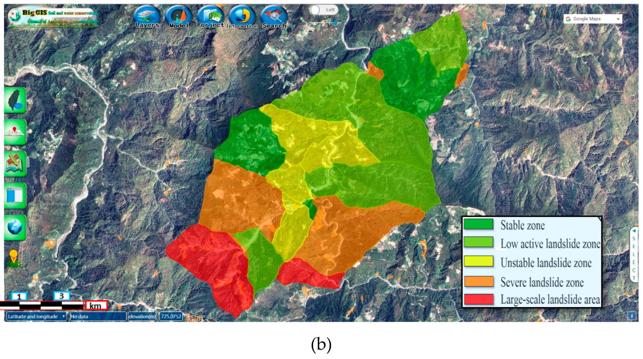
| Instability Levels | Grading Scale | Explanation |
|---|---|---|
| 1 | Stable area | Landslides never occurred, or only a few landslides occurred in this area with good natural restoration. The area is not easily destroyed. |
| 2 | Low active landslide area | Some landslides occur, but the landslide area is small, or the restoration after the landslide is obvious. |
| 3 | Unstable landslide area | Some landslides occur with massive landslide areas, or the landslide restoration is less obvious. |
| 4 | Severe landslide area | Massive landslide area, or an area where landslides occur frequently |
| 5 | Large-scale landslide area | An area where large-scale landslides occur |
| No | Area (ha) | Annual landslide Area (ha) | Instability Index | Instability Level | |||||||||||
|---|---|---|---|---|---|---|---|---|---|---|---|---|---|---|---|
| 2005 | 2006 | 2007 | 2008 | 2009 | 2010 | 2011 | 2012 | 2013 | 2014 | 2015 | 2016 | ||||
| 20894 | 11.23 | 0.37 | 0.00 | 0.26 | 0.00 | 0.00 | 0.00 | 0.00 | 0.00 | 0.00 | 0.00 | 0.00 | 0.00 | 0.01110 | 4 |
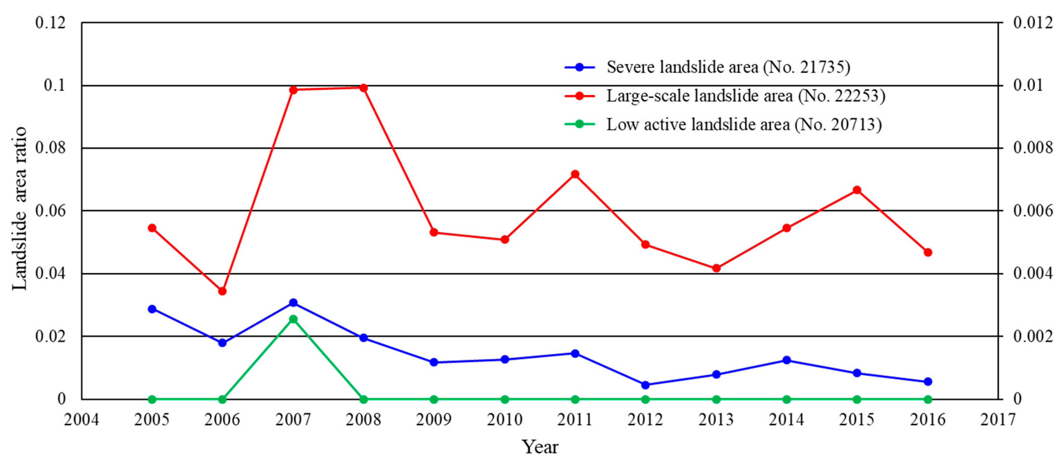
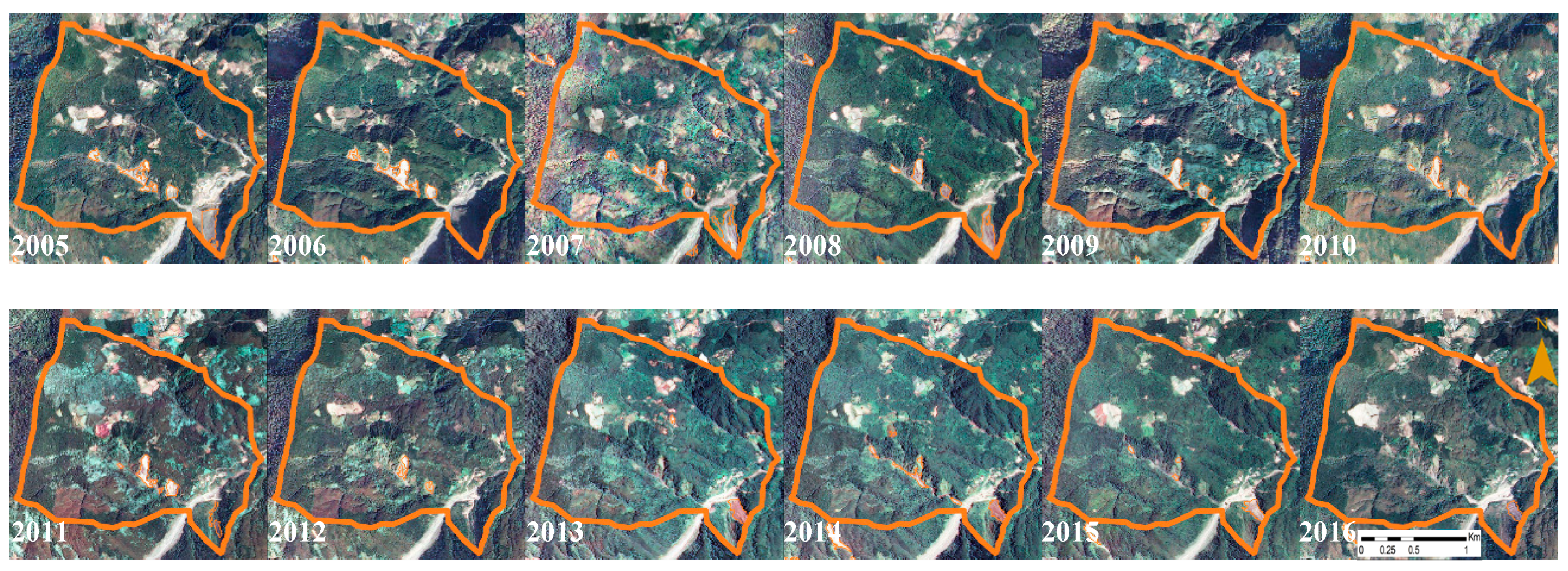
| 21735 | 324.94 | 9.36 | 5.81 | 9.98 | 6.36 | 3.81 | 4.11 | 4.75 | 1.46 | 2.56 | 4.05 | 2.71 | 1.80 | 0.00843 | 4 |
| 21897 | 372.25 | 18.69 | 11.93 | 14.92 | 11.09 | 11.71 | 11.19 | 10.75 | 7.65 | 7.41 | 10.33 | 9.08 | 3.93 | 0.01003 | 4 |
| 22062 | 108.72 | 1.13 | 1.11 | 1.52 | 1.04 | 2.51 | 1.14 | 0.95 | 0.00 | 0.00 | 1.30 | 0.54 | 0.70 | 0.00620 | 4 |
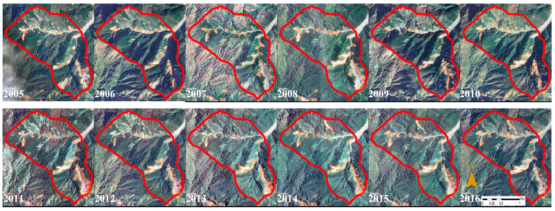
| 22253 | 298.04 | 16.24 | 10.24 | 29.37 | 29.58 | 15.86 | 15.17 | 21.38 | 14.67 | 12.43 | 16.27 | 19.87 | 13.98 | 0.02062 | 5 |
| 20610 | 150.57 | 0.53 | 0.42 | 0.28 | 0.00 | 0.00 | 0.00 | 0.00 | 0.00 | 0.00 | 0.27 | 0.16 | 0.00 | 0.00128 | 2 |
| 20759 | 11.29 | 0.18 | 0.00 | 0.29 | 0.33 | 0.00 | 0.00 | 0.21 | 0.00 | 0.14 | 0.00 | 0.00 | 0.00 | 0.01130 | 5 |
| 20928 | 163.21 | 0.47 | 0.10 | 0.00 | 0.00 | 0.19 | 0.00 | 0.00 | 0.70 | 0.71 | 0.36 | 0.36 | 0.38 | 0.00162 | 3 |
| 21045 | 89.31 | 0.32 | 0.01 | 0.00 | 0.00 | 0.00 | 0.00 | 0.00 | 0.00 | 0.00 | 0.26 | 0.00 | 0.00 | 0.00126 | 2 |
| 21084 | 106.23 | 0.11 | 0.00 | 0.00 | 0.00 | 0.00 | 0.00 | 0.00 | 0.00 | 0.00 | 0.00 | 0.00 | 0.00 | 0.00029 | 1 |
| 21100 | 155.90 | 1.84 | 1.10 | 1.42 | 0.00 | 0.00 | 0.39 | 0.00 | 0.10 | 0.20 | 0.00 | 0.00 | 0.00 | 0.00420 | 3 |
| 21191 | 270.83 | 1.16 | 0.23 | 0.50 | 0.00 | 0.51 | 0.18 | 0.70 | 0.47 | 0.29 | 1.27 | 1.09 | 0.83 | 0.00153 | 2 |
| 21414 | 145.41 | 2.46 | 0.00 | 1.47 | 0.54 | 0.00 | 0.27 | 0.00 | 0.00 | 0.10 | 0.42 | 0.70 | 0.00 | 0.00520 | 3 |
| 21704 | 277.64 | 0.83 | 0.00 | 0.32 | 0.36 | 0.21 | 0.00 | 0.00 | 0.20 | 0.00 | 0.11 | 0.00 | 0.00 | 0.00089 | 2 |
| 22057 | 76.77 | 4.40 | 5.41 | 5.81 | 4.12 | 3.36 | 5.82 | 2.34 | 1.40 | 2.07 | 0.23 | 0.00 | 0.00 | 0.02899 | 5 |
| 22061 | 7.39 | 0.12 | 0.12 | 0.17 | 0.00 | 0.00 | 0.00 | 0.00 | 0.00 | 0.00 | 0.00 | 0.00 | 0.00 | 0.00853 | 4 |
| 22191 | 117.37 | 0.06 | 0.21 | 0.39 | 0.00 | 0.31 | 0.00 | 0.00 | 0.00 | 0.00 | 0.00 | 0.00 | 0.00 | 0.00120 | 2 |
| 21628 | 73.18 | 0.00 | 0.16 | 0.00 | 0.00 | 0.39 | 0.00 | 0.00 | 0.77 | 0.00 | 0.00 | 0.00 | 0.00 | 0.00327 | 3 |
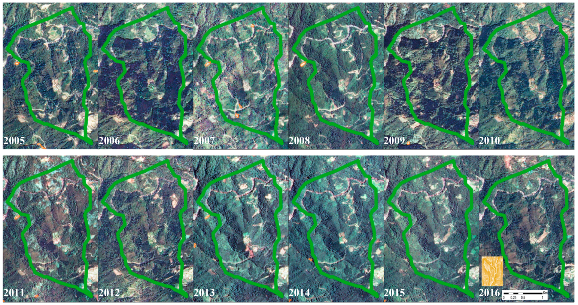
| 20713 | 175.81 | 0.00 | 0.00 | 0.45 | 0.00 | 0.00 | 0.00 | 0.00 | 0.00 | 0.00 | 0.00 | 0.00 | 0.00 | 0.00073 | 2 |
| 21512 | 58.93 | 0.00 | 0.00 | 0.17 | 0.00 | 0.00 | 0.00 | 0.12 | 0.00 | 0.00 | 0.00 | 0.00 | 0.00 | 0.00098 | 2 |
| 21793 | 10.98 | 0.00 | 0.00 | 0.00 | 0.00 | 0.00 | 0.01 | 0.00 | 0.00 | 0.00 | 0.00 | 0.00 | 0.00 | 0.00026 | 1 |
| 21320 | 207.05 | 0.00 | 0.00 | 0.00 | 0.00 | 0.00 | 0.00 | 0.00 | 0.00 | 0.00 | 0.20 | 0.22 | 0.00 | 0.00040 | 1 |
© 2019 by the authors. Licensee MDPI, Basel, Switzerland. This article is an open access article distributed under the terms and conditions of the Creative Commons Attribution (CC BY) license (http://creativecommons.org/licenses/by/4.0/).
Share and Cite
Liu, C.-C.; Ko, M.-H.; Wen, H.-L.; Fu, K.-L.; Chang, S.-T. Instability Index Derived from a Landslide Inventory for Watershed Stability Assessment and Mapping. ISPRS Int. J. Geo-Inf. 2019, 8, 145. https://doi.org/10.3390/ijgi8030145
Liu C-C, Ko M-H, Wen H-L, Fu K-L, Chang S-T. Instability Index Derived from a Landslide Inventory for Watershed Stability Assessment and Mapping. ISPRS International Journal of Geo-Information. 2019; 8(3):145. https://doi.org/10.3390/ijgi8030145
Chicago/Turabian StyleLiu, Cheng-Chien, Ming-Hsun Ko, Huei-Lin Wen, Kuei-Lin Fu, and Shu-Ting Chang. 2019. "Instability Index Derived from a Landslide Inventory for Watershed Stability Assessment and Mapping" ISPRS International Journal of Geo-Information 8, no. 3: 145. https://doi.org/10.3390/ijgi8030145