Mr4Soil: A MapReduce-Based Framework Integrated with GIS for Soil Erosion Modelling

Abstract

A soil erosion model is used to evaluate the conditions of soil erosion and guide agricultural production. Recently, high spatial resolution data have been collected in new ways, such as three-dimensional laser scanning, providing the foundation for refined soil erosion modelling. However, serial computing cannot fully meet the computational requirements of massive data sets. Therefore, it is necessary to perform soil erosion modelling under a parallel computing framework. This paper focuses on a parallel computing framework for soil erosion modelling based on the Hadoop platform. The framework includes three layers: the methodology, algorithm, and application layers. In the methodology layer, two types of parallel strategies for data splitting are defined as row-oriented and sub-basin-oriented methods. The algorithms for six parallel calculation operators for local, focal and zonal computing tasks are designed in detail. These operators can be called to calculate the model factors and perform model calculations. We defined the key-value data structure of GeoCSV format for vector, row-based and cell-based rasters as the inputs for the algorithms. A geoprocessing toolbox is developed and integrated with the geographic information system (GIS) platform in the application layer. The performance of the framework is examined by taking the Gushanchuan basin as an example. The results show that the framework can perform calculations involving large data sets with high computational efficiency and GIS integration. This approach is easy to extend and use and provides essential support for applying high-precision data to refine soil erosion modelling.

1. Introduction

Soil erosion models are a useful tool for predicting the amount of soil erosion, guiding the allocation of soil and water conservation measures, and optimizing the utilization of water and soil resources in basins. As soil erosion has become a global environmental problem influenced by both natural and human factors, soil erosion modelling is a research topic that has drawn widespread attention around the world. Since the last century, researchers have established various soil erosion models from the prototype experiments and observations. In the early stages, the empirical statistical models were developed based on statistical analyses of observational data collected in plot and small watersheds with sheet and rill erosion. Examples of empirical models include the universal soil loss equation (USLE) [1] or its derivatives (e.g., the revised universal soil loss equation, RUSLE) [2] and Chinese soil loss equation (CSLE) [3,4]. These models have often been applied for on-site soil erosion estimates without considering the spatial heterogeneity of the soil erosion process [5]. With advances in geographic information system and remote-sensing technology, models and predictions of soil erosion have been developed from empirical statistical models. Now, many models are spatially distributed or physically based models. The spatially distributed models account for watershed heterogeneity, as reflected by the land use, soil types, topography, and rainfall, measured in the field or estimated through digital elevation models (DEMs) or remote-sensing images, and estimates of the sediment yield are generated in various spatial domains [6]. The Water Erosion Prediction Project (WEPP) model is a well-known and commonly used example; it is a process-based, spatially distributed parameter, and continuous simulation and erosion prediction model [7]. From a computational perspective, soil erosion models, especially spatially distributed models, all involve raster data, such as precipitation, topographic, soil, and vegetation data. Moreover, such models include various computational subprocesses and are characterized by large data volumes and intensive computational tasks. These computations, which involve exceptionally detailed high-resolution soil erosion modelling, are limited by the data storage and computing speed of the corresponding computing platforms.

In recent years, with the rapid development of information technology, massive amounts of data have been produced in different fields. To analyse and utilize these big data resources, related parallel computing methods must be used. Conventional methods usually include high-performance computing platforms (HPCs) and parallel programming models, such as message-passing-interface (MPI) and open multi-processing (OpenMP), to split the computational tasks and combine the final computing results [8]. Additionally, with the development of graphics processing hardware, the ability of graphics processing units (GPUs) has been improved, leading to the development of the computing unified device architecture (CUDA) and open computing language (OpenCL) parallel computing framework [9]. In the GIS and Remote Sensing (RS) field, Guan et al. [10] developed the parallel raster processing library (pRPL) for raster analysis in GIS. Integrated data management class, a Geospatial Data Abstraction Library (GDAL)-based raster data Input/Output (I/O) mechanism and a static and dynamic load-balancing mode were added to pRPL 2.0. Miao et al. [11] implemented a parallel GeoTIFF I/O library (pGTIOL) based on an asynchronized I/O mechanism that displayed better performance than using GDAL as the I/O interface. Both the pRPL and pGTIOL are MPI-enabled libraries. Qin et al. [12] designed and implemented a set of parallel raster-based geocomputation operators (PaRGO) to overcome the poor transferability of parallel programs. The PaRGO is compatible with three types of parallel computing platforms: GPUs, the MPI, and OpenMP. This approach makes the details of the parallel programming and the parallel hardware architecture transparent to users. Zhang et al. [13] introduced a parallel approach to quadtree construction and implemented on general purpose GPUs. A performance test yielded a significant speedup for the studied tasks. Although these libraries rely on parallel computing capabilities for raster data processes, they are limited by particular hardware environments (GPU/multi central processing unit (CPU)) and software frameworks, making them difficult to scale or expand.

The MapReduce parallel computing model for big data analysis developed by Google performs the parallel processing of massive amounts of data through cheaper server clusters [14]. This model has advantages such as few hardware requirements, rapid scaling, and easy modelling [15]. After the launch of the Hadoop open-source platform, MapReduce has been extensively used in big data processing and has formed a complete ecosystem [16]. There are several platforms for spatial big data processing and analysis such as Hadoop-GIS [17], SpatialHadoop [18], ST-Hadoop [19], GeoSpark [20], MrGeo [21], GIS Tools for Hadoop [22], Geotrellis [23] and others. In specific areas of spatial data analysis, a series of Hadoop application cases has also emerged. In the climate data analysis area, Li et al. [24] proposed a spatiotemporal indexing method that can effectively manage and process large climate datasets using the MapReduce programming model in the Hadoop platform and built a high-performance query analytical framework for climate data using the Structured Query Language (SQL) style query (HiveQL) [25]. Gao et al. [26] harvest crowd-sourced gazetteer entries running on a spatially enabled Hadoop cluster. Similar research areas include atmospheric analysis [27], large-scale Light Detection and Ranging (LiDAR) data analysis [28], remote sensing [29], trip recommendation [30], and others [31,32]. These platforms and cases are suitable for different spatial data and can be applied in different applications and domains. In this paper, we focus on integrating the Hadoop platform with GIS for parallel computing involving soil erosion modelling.

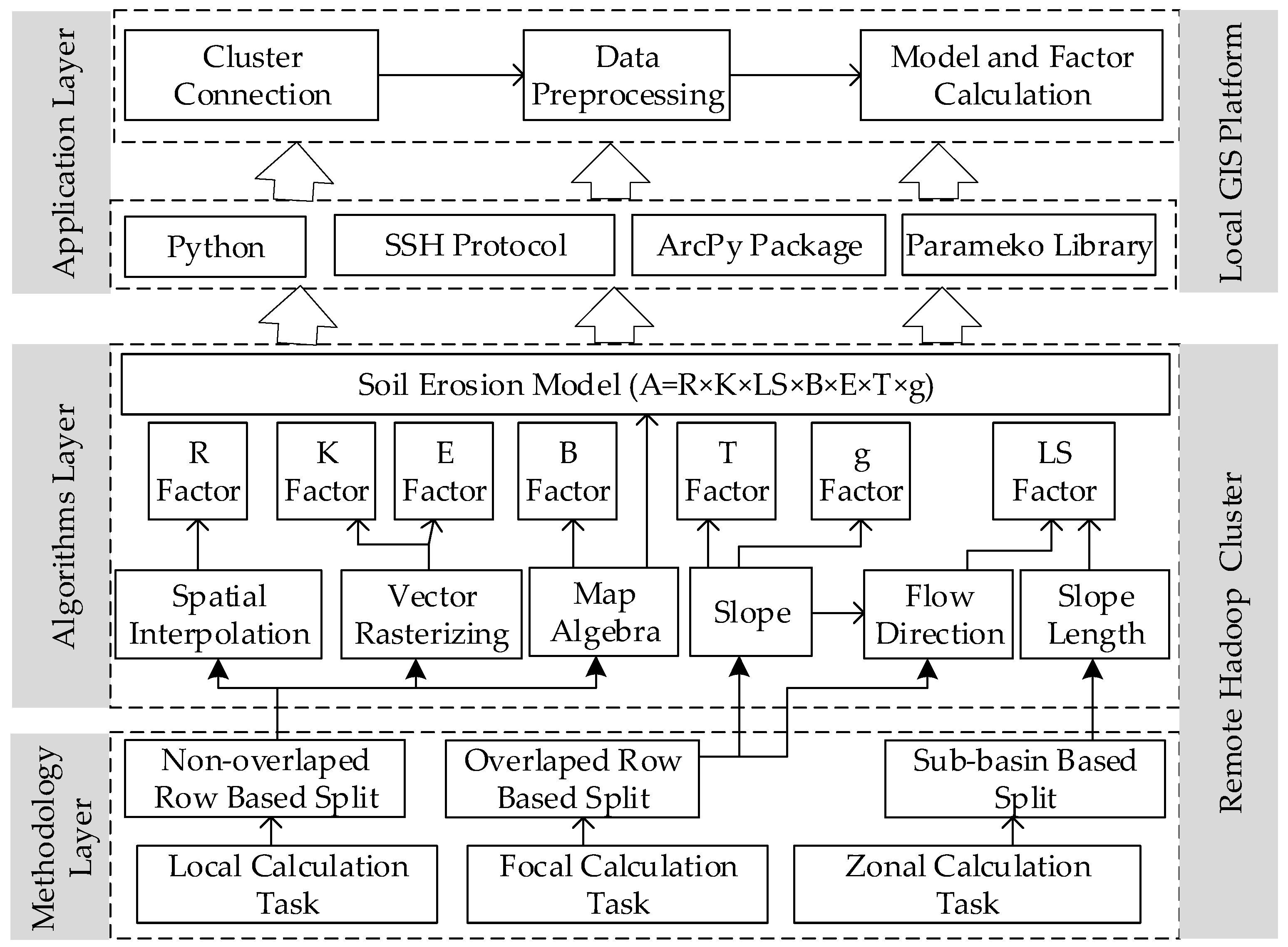
With the rapid development of geographic information technology, three-dimensional laser scanning technology can be applied to obtain high-precision geographic information data such as DEM data at the basin scale. As the resolution of raster data has increased, the data volume has exponentially grown, thus demanding a higher requirement for refined large- to medium-scale soil erosion modelling in basins. The Hadoop parallel computing platform can be used to build a parallel computing framework for soil erosion modelling and then be tightly integrated or coupled with GIS for refined soil erosion modelling. In this study, we implemented a parallel computing framework (Mr4Soil) integrated with the GIS platform. The framework includes three layers: the methodology layer, algorithms layer, and application layer. We designed two types of parallel computing strategies as rows-oriented and sub-basin-oriented methods using a spatially distributed model for annual sediment yield associated with soil erosion. We developed parallel algorithms for soil erosion modelling in the Hadoop platform based on the MapReduce parallel computing method. A series of experiments showed that Mr4Soil yielded better performance than other conventional serial programming methods. Thus, the proposed approach provides a solution for the refined soil erosion modelling on the Hadoop platform, which is integrated with a GIS platform.

2. Mr4Soil Framework Overview

2.1. Model Description

This study uses the annual sediment yield model for the large- to medium-scale basins developed by the Yellow River Institute of Hydraulic Research. Adopting Chinese Soil Erosion Equations and implementing a spatially distributed method, the model is based on the spatial discretization of the basin and comprehensively considers influences such as precipitation, soil, and topography. Therefore, the model is suitable for estimating the annual sediment yield of large- to medium-scale basins. The model formula [33] is as follows:

$$A_i=R\times K\times LS\times B\times E\times T\times g$$

(1)

where A is the annual soil erosion in raster cell i; R is the rainfall erosivity, which is calculated at each rain gauge station in the basin by using long-term mean monthly rainfall data; K is the soil erodibility factor, and E is the soil and water conservation practice factor. The values of K and E are related to different soil types and the distribution of soil and water conservation engineering measures in the river basin. Among them, the K factor mainly considers the composition of soil organic carbon and the particle sizes of different soil types, and E is estimated using statistical data in different administrative regions in the river basin. LS is a topographic factor that can be calculated using a CSLE model based on the extracted slopes and slope length parameters. B is a vegetation factor that reflects the influence of surface vegetation on soil erosion. B can be estimated for different land uses and vegetation coverages. T is the tillage factor, which reflects the relationship between soil erosion and farming methods, and it can be determined according to the reduction in soil erosion as a result of contour ploughing under different slope conditions. Additionally, g is the gully erosion factor, which reflects the degree of erosion by surface runoff in the river basin, and the annual mean value can be calculated by considering the slope conditions. The calculation methods for each factor are shown in

Table 1. Soil erosion model factors calculation method.

Factors	Calculation Method	Parameters Notes
R	$R=0.183F_F{}^{1.996},F_F=\frac{1}{N}{\displaystyle \sum _{i=1}^N}({\displaystyle \sum _{j=1}^{12}}{P}_{i,j}^2)/({\displaystyle \sum _{j=1}^{12}}{p}_{i,j})$	$P_{i,j}$ is the rainfall of i year, j months, N is the number of years
K	$K=\left\{0.2+0.3\exp \left[0.0256SAN\left(1-\frac{SIL}{100}\right)\right]\right\}\times {\left(\frac{SIL}{CLA+SIL}\right)}^{0.3}\times$ $\left[1.0-\frac{0.25C}{C+\exp \left(3.72-2.95C\right)}\right]\times \left[1.0-\frac{0.7SN1}{SN1+\exp \left(-5.51+22.9SN1\right)}\right]$	SAN/SIL/CLA/C are the corresponding soil types of sand grains, powders, sticky grains and organic carbon content, SN1 = 1 − SAN/100
LS	$S=\{\begin{array}{l}10.8sin\theta +0.03, \theta <5°\\ 16.8sin\theta -0.50, 5°\le \theta <10°\\ 21.9sin\theta -0.96, \theta \ge 10°\end{array}$	$\theta$ is the slope of the raster cell
	$L={(\lambda /22.1)}^m$; $m=\{\begin{array}{l}0.2, \theta \le 1°\\ 0.3, 1°<\theta \le 3°\\ 0.4, 3°<\theta \le 5°\\ 0.5, \theta >5°\end{array}$	$\lambda$ is the slope length
B	$f=\frac{NDVI-NDV{I}_{\min }}{NDVI-NDV{I}_{\max }}$	f is vegetation cover ratio, NDVI is normalized vegetation index, B value is shown in Table 2
E	$E=\left(1-\frac{\alpha S_t}{S}\right)\times \left(1-\frac{\beta S_d}{S}\right)\times \left(1-\frac{\omega N_{d1}+ϵN_{d2}}{A\times S}\right)$	S/Sd/S are the area of terraced fields, silt storage dams and total land, α/β are the sand reduction coefficient of terraced fields and silt storage dams, Nd1/Nd2 and $\omega$/$ϵ$ are the number and sand reduction quota of sand or check dam, A is the annual erosion modulus
T	$T=\{\begin{array}{c}1.000, \theta =0°\\ 0.100, 0°<\theta \le 5°\\ 0.221, 5°<\theta \le 10°\\ 0.305, 10°<\theta \le 15°\end{array}$, T$=\{\begin{array}{c}0.575, 15°<\theta \le 20°\\ 0.705, 20°<\theta \le 25°\\ 1.000, \theta \le 25°\end{array}$	$\theta$ is the slope of raster cell
g	$G=1+1.60\sin (\theta -15)$	$\theta$ is the slope of raster cell

and

Table 2. B factor values for different land-use and vegetation cover ratio.

Landuse	Vegetation Coverage (%)	B Factor Value
Forest/grass	0~20	0.10 (forest)	0.45 (grass)
	20~40	0.08 (forest)	0.24 (grass)
	40~60	0.06 (forest)	0.15 (grass)
	60~80	0.02 (forest)	0.09 (grass)
	80~100	0.004 (forest)	0.043 (grass)
Construction	-	0.9
Water	-	1
Arable	-	0.23

.

From a computational perspective, this model involves a large amount of raster analysis computations. According to the range of raster neighbourhoods involved in the analysis, the computing tasks can be classified into three types: (1) local operations, which use the calculation results of the current raster cell are independent of other cells and only related to the information about itself or raster cell at the same position in other layers; (2) focal operations, which use the calculation results of the current raster cell are related to neighbouring cells within a certain range, in which a typical neighbourhood is a 3 × 3; and (3) zonal operations, which use the calculation results of a single cell that affect those of other cells, and the affected range is an irregular zone (e.g., a sub-basin). The aforementioned tasks affect data splitting strategies for model parallel computing.

2.2. Framework Overview

According to the structure and computational requirements of the soil erosion model, the Mr4Soil parallel computing framework is designed, as shown in Figure 1. The framework includes three layers such as the methodology layer, algorithm layer, and application layer. In the methodology layer, the data splitting strategies for splitting by row and splitting by sub-basin are designed according to the three types of operational tasks first. Then we abstract six parallel computing operators in the algorithm layer. The operators consist of (1) local operation parallel operators, including the spatial interpolation, vector rasterization, and map algebra operators, which are suitable for the strategy of non-overlapping splitting by row and are used to calculate R, K, E, B, and soil erosion; (2) focal operation parallel operators, including the slope analysis and flow direction analysis operators, which are suitable for the strategy of overlapping splitting by row and are used to calculate T, g, and LS; and (3) zonal operation parallel operators, mainly involving the slope length extraction operator, which is suitable for the sub-basin splitting strategy and is used to calculate the slope length of LS. The six parallel computing operators are implemented using the Hadoop platform MapReduce library. These operators can be called during soil erosion modelling. From six parallel computing operators, functions of the model parameters and the model computations are developed and compiled as Java jar file to execute on the Hadoop platform. The methodology and algorithm layer are in the Hadoop platform. To integrate the soil modelling parallel functions with GIS platform, tools for cluster connection, data pre-processing, and model computation are implemented using the ArcPy library, Secure Shell (SSH) remote access protocol, and Python language. The remote execution of parallel computing functions in the soil erosion model is achieved in the ArcGIS environment of the local machine.

2.3. Data-Splitting Methods

The Hadoop platform uses the MapReduce programming model to perform distributed computing on big data. This model provides a complete set of programming interfaces for developing distributed application programs. By splitting the input data, computations are performed for each subslice by the Mapper process, and the computational results for the subslices are then combined in a reducing process [34]. Ideally, the processing among various computing nodes after data splitting should be independent of each other to minimize the cost of communication among nodes. According to this requirement and the calculation task characteristics of the soil erosion model, we designed two data splitting strategies as follows.

(1) Split by row. In this splitting strategy, according to the number of computational nodes in parallel clusters, the raster data are split according to the number of rows. The raster data in the corresponding row are assigned to the corresponding computing node. The number of raster rows assigned to each node is calculated using Equation (2).

$$h=\{\begin{array}{c}RC/N if mod\left(RC,N\right)=0\\ int\left(RC/N\right)+1 if mod\left(RC,N\right)\ne 0\end{array}$$

(2)

where h is the number of raster data rows for each subslice, RC is the total number of rows of raster data, N is the number of computational nodes, and the mod is a residual function. For local operations, the calculation results for a raster cell are not related to and do not affect the results of other cells. Therefore, there is no need to consider the data in adjacent cells after the split, meaning that there is no overlap in splitting (Figure 2). For example, the map algebra operation can be finished with the non-overlap data splitting method because each raster cell is calculated independently of its neighbourhood raster. After the raster data input, the raster is divided into non-overlap segmentation according to the row and assigned to the calculation node in the cluster. Then each node can perform the corresponding algebraic operations on the allocated data rows at the same time. Figure 2 is an example of the multiplication of each raster cell.

For neighbourhood operations, the neighbourhood ranges are different among computations. To ensure that all cells in the corresponding neighbourhood are read at the same computational node, h must be expanded on the basis of non-overlapping splitting. Assuming that the width of a neighbourhood is W, the upper and lower boundaries of the neighbourhood are each $\left(W-1\right)/2$ rows away from the centre, meaning that there is overlapping splitting. Figure 3 is an example of summing the range of the 3 × 3 neighbourhood of each raster cell. With an overlap segmentation strategy, the rows of raster data allocated to each compute node are overlapped, thereby completing independently at each node. The cell in the 3 × 3 window is calculated, and finally, the results of each node are combined and output.

(2) Split by sub-basin. In the calculation of some parameters in the soil erosion model (such as the slope length factor), the calculation results of the corresponding raster cell are related to the values of other cells within a certain range. In contrast to neighbourhood operations, this range is an irregular area (such as a sub-basin). The parallel computation of these factors is performed using the sub-basin splitting strategy. That is, using DEM data in the basin, sub-basins are divided according to watershed lines; then, the sub-basins are assigned to the corresponding nodes according to their spatial adjacent relations (Figure 4). When the basin is divided into sub-basins, the sub-basins can be properly merged or subdivided under the correct flow accumulation in a watershed. To avoid large differences in the data volume of nodes, which influences the overall computational efficiency, the sub-basin area assigned to each node should be roughly equal so that the computing load of each node is balanced. As shown in Figure 4, the watershed is divided into 67 sub-basins. Since the cluster has four computing nodes, these sub-basins are merged according to the adjacent relationship to obtain four polygon ranges. The point in polygon spatial relationship is identified for each raster cell and get the polygon ID value. Then the cells are assigned to different computing nodes according to corresponding polygon ID to complete parallel computing tasks. Using the data input class Nlineinputformat and Keyvalueiputformat class in the Hadoop platform MapReduce library [35], the input raster data could be partitioned by configuring the raster rows, worker nodes, and the sub-basin boundary parameters.

3. Parallel Algorithms Design

The parallel algorithms of model consist of 3 levels: (1) the parallel model operators, which are used to define the basic analysis algorithm; (2) the parallel factor algorithms, which are used to achieve parallel computing of different model factors; and (3) the parallel model algorithm, which is used to calculate soil erosion according to Equation (1). The parallel model operators are at the bottom level. The model factor and model calculations can be completed by calling the corresponding operators. Based on the data structure definition and data preprocessing, this section focuses on the algorithm design for parallel model operators.

3.1. Data Structure and Data Preprocessing

The Hadoop platform supports the reading and writing of structured text data and binary data. To simplify the calculations, the (key, value) pair in text format is applied to define the data structure involved in parallel model computing. There are two types of input data used in model computations: vector and raster data. Vector data mainly include rainfall data collected at rain gauge stations (point) in the basin, soil type data, soil and water conservation measure data (polygon), and sub-basin boundary data (polygon). The volume of these data is relatively small, and there is no need for splitting in the calculation. Vector data are converted into a text format supported by the Hadoop platform. In this study, vector data are converted into GeoCSV format. The geographic entity code is used as the key. Spatial data, which are stored in well-known text (WKT) format, together with property data are used as the value and can be directly read by the Hadoop distributed file system (HDFS) API and used in calculations. The raster data mainly include the basin DEM, land-use data, and normalized difference vegetation index (NDVI) data. First, these data are converted into two-dimensional text data. Then, two types of (key, value) pairs are defined: (1) an entire row is used as a (key, value) pair, where key is the row number and value is the set of the corresponding raster cell values of the row; and (2) a raster cell is used as a (key, value) pair, where the row number and column number of a raster cell are defined as the composite key, and the value of the raster cell is defined as the value. The raster data are preprocessed, and the corresponding (key, value) pairs in text format are generated and used as input data in different parallel algorithms.

3.2. Parallel Algorithms Based on the Row-Splitting Method

The row-splitting method is suitable for local and neighbourhood operations. By using an entire row as a (key, value) pair for input data, the calculation process includes 2 steps: (1) in the map step, the splitting function is defined according to the key of the row of the input raster data, and the raster data row is assigned to the corresponding computing nodes; (2) in the reduce step, based on the different analysis algorithms, calculations are performed involving the slices of data rows. The results of the slices are sorted according to the key, combined and output. In local operation tasks, there is no need to consider the overlap among slices. The (key, value) pair raster data in text format can be directly used in calculations. In focal operation tasks, the corresponding raster rows must be duplicated in the first and last rows of each slice according to the size of the neighborhood windows. Herein, the spatial interpolation parallel operators based on the inverse distance weighting (IDW) method are used as an example. The input parameters of the parallel algorithm include: (1) the observation station data as GeoCSV, which stores the station position and its observation value. The data volume is small and can be used for each computational node without data splitting. (2) The row key-value pair raster data in text format (the initial value of a raster cell is set to −1). The key is row number, and the value is the cell list of the row. Spatial interpolation is the process of calculation each raster cell value based on the observation station data. The calculation steps are as follows (Figure 5).

(1) Data input. Read the key-value text of the row, and parse the row number and the raster cell list; read and parse the GeoCSV text to get the station position and value.

(2) Data splitting. The number of raster rows allocated by each node is calculated according to formula (2) and cluster size, and then the rows are assigned to the corresponding computational node by customizing the MapReduce splitter (partitioner) to perform non-overlapping row segmentation according to the line number.

(3) Data parsing and distance calculation. The coordinates of the raster cell center are calculated from the cell width and row/column number. The distance from the raster cell and all of the station are measured to generate a set {(d_i, v_i)}, where d_i is the distance and v_i is the observation value.

(4) Spatial interpolation. According to the IDW interpolation method, the interpolation points within a certain range of the current raster cell by the distance are selected. The interpolation calculation is weighted by the distance, and the values of the corresponding raster cells (c_ij) are updated.

(5) Output. A list is generated based on the interpolation result of each raster cell of the row, and written to the HDFS along with the row number (Figure 6).

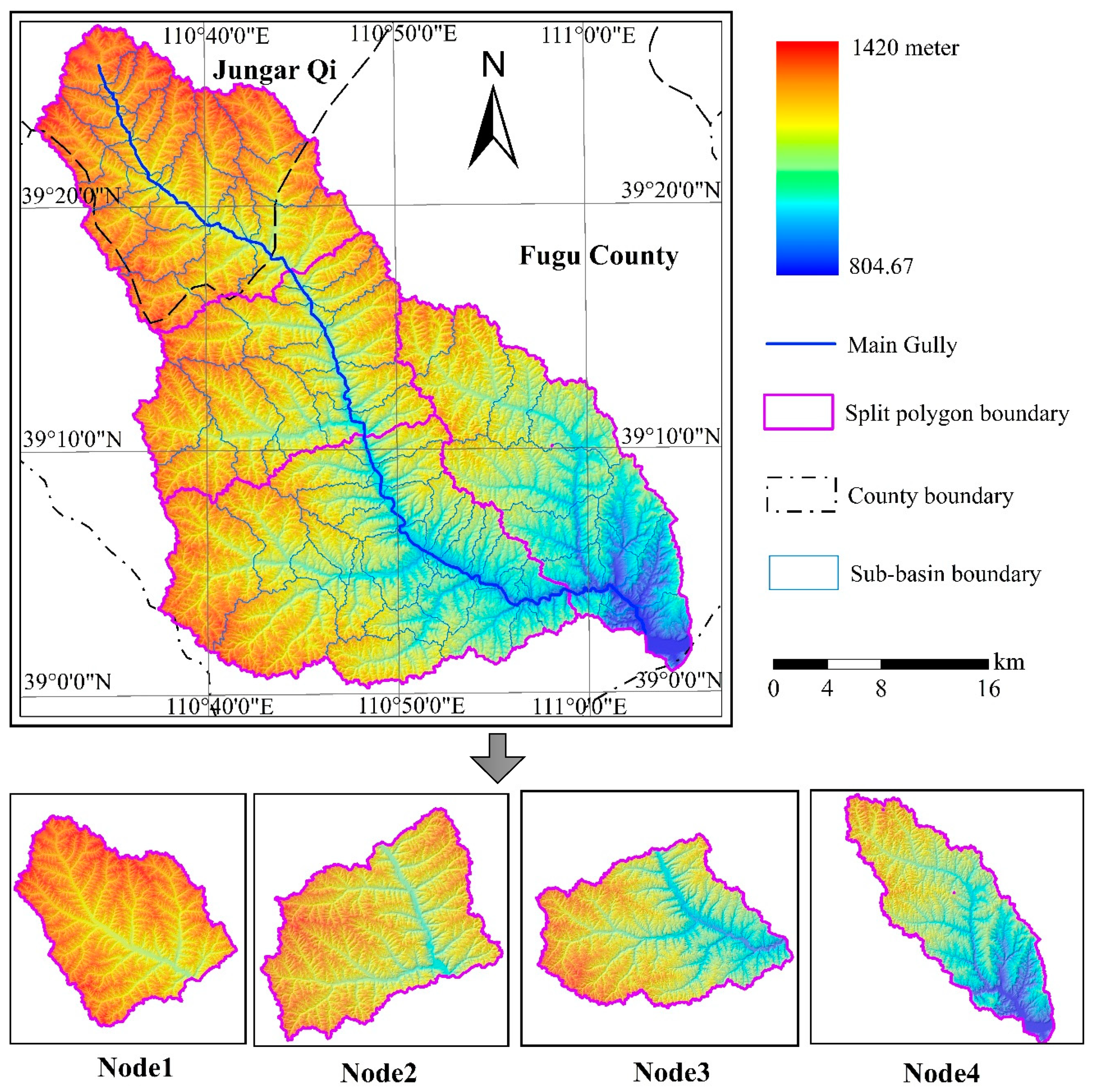
3.3. Parallel Algorithms Based on the Sub-Basin Splitting Method

Among the topographic factors of the model, slope length is a key parameter that affects soil erosion. The serial computing process of the slope length includes steps such as slope and flow direction determination, flow accumulation, cut-off detection, cell slope length determination, and cumulative slope length calculations. Among these steps, the flow accumulation and cumulative slope length calculation steps involve cumulative process and different raster cells according to the flow path. Parallel computations cannot be directly performed following the row-splitting strategy. The flow paths include two subsets, namely, the flow paths in each sub-basin and the main gully in the basin. Flow accumulation can be calculated independently in the sub-basins, whereas flow accumulation in the main gully of the basin involves fewer raster cells, and thus, no data splitting is needed. Flow accumulation in the main gully can be completed directly in the reduce phase after the sub-basin calculations are performed. Based on the analysis above, the sub-basin splitting strategy can be used to parallelize slope length extraction. The algorithm can be implemented by using the master-slave parallel computing processes in MapReduce. Slave computing processes mainly refer to subprocesses in which only some of the data are involved and no global data need to be considered. The computing results serve as intermediate data that are input into the master computing process. The input data of the algorithm are the raster-based (key, value) pairs in text format (DEM, slope and flow direction) and the GeoCSV data of the splitting polygon which store the polygon ID and boundary coordinates. The main steps are as Figure 7 shown.

(1) Data input. Read the key-value text of the raster, parse the row and column number of the cell and calculate the cell center coordinates. Read and parse the GeoCSV text to get the splitting polygon ID and boundary coordinates.

(2) Splitting polygon identification and data splitting. The ray casting method for point-in-polygon testing is used to determine the splitting polygon in which the cell is located, and get the polygon ID to customize the partitioner to perform sub-basin splitting. Then the raster cells are sent to different computational nodes.

(3) Slope length calculation for cells in the sub-basin. For each raster cell assigned to the worker node, the flow accumulation, cut-off detection, cell slope length, and cumulative slope length are calculated using the serial calculation method of the slope length; and output the cumulative slope length of each cell.

(4) Slope length calculation for cells in the main gully. According to the result of the flow accumulation in (3), the main gully cell is determined. The flow accumulation, cut-off detection, cell slope length, and cumulative slope length of these cells is computed by the same process as step (3).

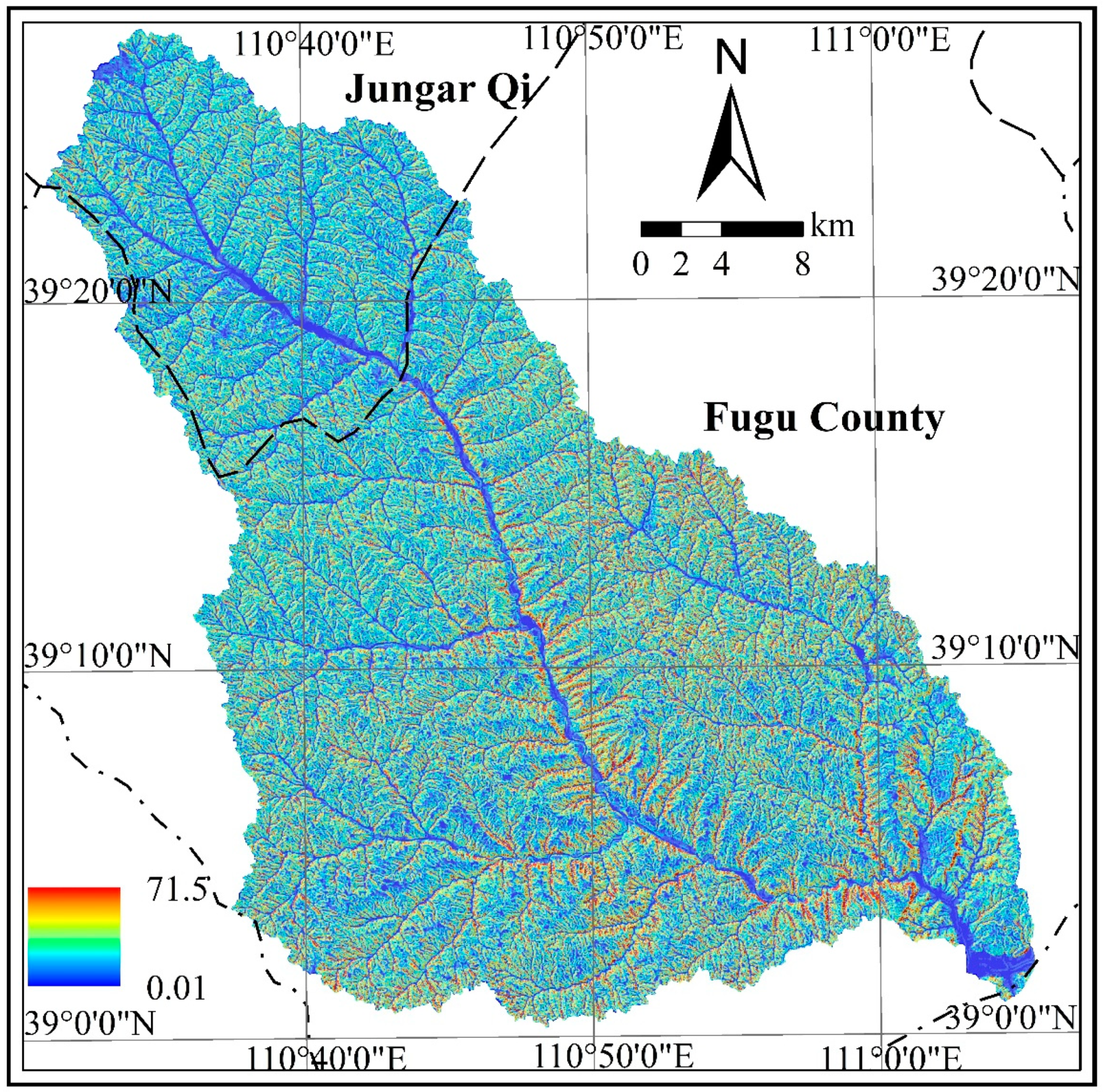
(5) Combination and output. The slope length for cells in the sub-basin and the main gully is merged with the rules as follows: if the cell is in the main gully, the slope length generated by step (4) are the slope length value of the cell; otherwise is the step (3). The slope length of the complete watershed is written to HDFS. The LS factor is then calculated according to the corresponding method in Table 1 (Figure 8).

According to the two parallel algorithms described above, spatial interpolation, vector rasterization, map algebra, slope gradient, flow direction, and slope length operations are implemented using the MapReduce programming interface. Based on the model factors and model structure, the corresponding parallel operators are called to calculate model factors and perform model calculations in the basin.

4. Toolbox Development Integrated with Geographic Information System (GIS)

The Hadoop platform is operated on a Linux parallel computing cluster that consists of multiple computing nodes. Thus, multiple Linux and Hadoop commands must be executed to complete the corresponding computing tasks. The process also involves uploading or downloading model data to/from clusters, which complicates the parallel computing tasks in the model described above. To improve the usability and ease of operation of parallel computing functions in the model, a geoprocessing toolbox is compiled from the model parallel computing functions using a Python script based on the ArcGIS platform. This toolbox allows for the direct calling and the visualization of the computational results in the ArcGIS platform, thus achieving the integration of the parallel computing functions of the model with ArcGIS.

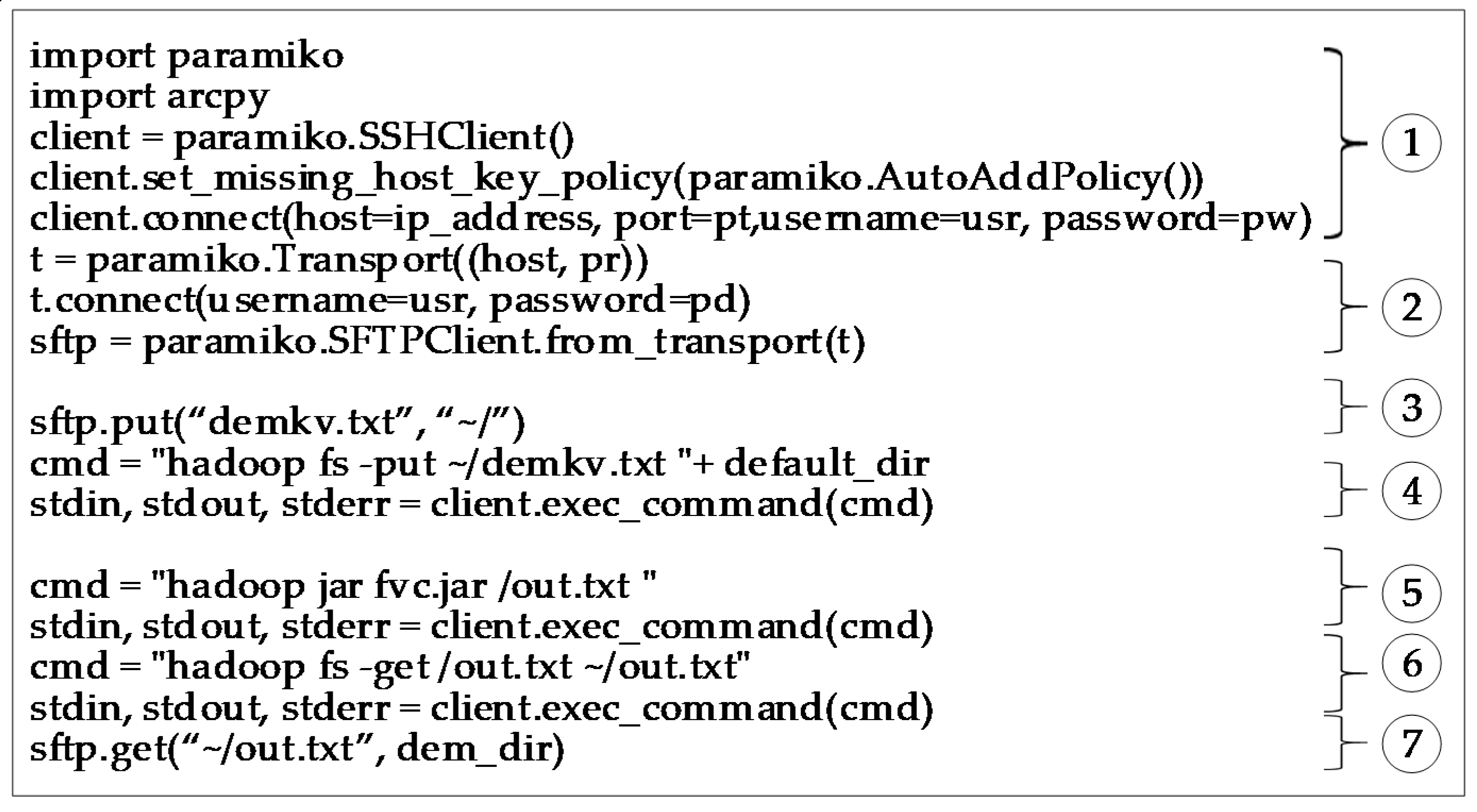
As the toolbox runs on the ArcGIS platform of the local machine, the SSH (secure shell) protocol is used to complete the communication between the local machine and the remote cluster. The SSH protocol is a method of securing remote login operations from one computer to another. The Linux platform provides an SSH access protocol for remote login and other operations. On the Windows platform of the local machine, we use Paramiko, an SSH access library in Python, to interact with the Linux platform. Paramiko provides two types of objects: SSHClient, which is used to implement login to remote hosts and perform various command operations, and SFTPClient, which is used to implement upload and download files. The calculation pipeline of the Mr4Soil is shown in Figure 9. First, according to the internet protocol (IP) address of the remote host, network port, and other information, a user can connect to the master node of the Hadoop cluster via the SSHClient and SFTPClient objects on the local machine and then convert the data in GIS format to GeoCSV format or a key-value text file through the ArcPy package. Second, the converted data can be uploaded to the master node by calling the put method of SFTPClient. Next, these files on the master node are transferred to the HDFS of the Cluster using Hadoop platform file operation command and the EXEC_COMMAND function of SSHClient. Then, the corresponding MapReduce program is executed using the Hadoop platform Java Archive (JAR) operation command in the same way to compute the various factors and perform soil erosion calculations. Finally, the user can download the results to the local machine and convert them to GIS format and use the ArcGIS platform for browsing and viewing.

There are three tools in the application layer of the framework (Figure 10a). (1) The cluster connection tool. Using the Paramiko module and the SSH protocol to login to the cluster remotely, files can be uploaded and downloaded through SFTP (SSH file transfer protocol). For a flexible connection method, the cluster login IP and network service port are set as login parameters. Parameter passing occurs through the ArcGIS customization tool. Remote login to the clusters in the Windows environment is then achieved (Figure 10b). (2) The data preprocessing tool. This tool is mainly used to achieve two-way interoperability between native GIS data and text data for the HDFS of the cluster. The tool converts GIS vector data to GeoCSV format and GIS raster data to key-value pair text format using the data access and conversion functions in ArcPy. Then, the data processing tool uploads the data to HDFS to read in model operations through the SFTPClient object of the Paramiko library (Figure 10c). (3) The model computing tool. Model computation is a process based on the calculation function of each model factor and soil erosion. This process compiles these functions into JAR packages, uploads the packages to the cluster master nodes, and calls the packages. The model computing tool encapsulates this process. After the user specifies the computing task, the corresponding JAR package is executed by the SSHClient object, thereby completing the model computation and writing the results to the HDFS (Figure 10d).

5. Experiment and Test

5.1. Data Sources and Experimental Environment Configuration

The Loess Plateau is an area of severe soil erosion in China. This paper selects the Gushanchuan basin on the Loess Plateau as a typical research area (Figure 11) for Mr4Soil application and testing. Gushanchuan is a primary tributary on the right bank of the middle reaches of the Yellow River. It originates in Jungar Qi, Inner Mongolia, and flows through Jungar Qi and Fugu County, Shaanxi Province, and into the Yellow River in Fugu Town. The length of the main channel is 79.4 km, and the average slope ratio is 5.4‰. The Gushanchuan basin (E110°32′24″~E111°05′24″, N39°00′00″~N39°27′36″) is located on the southeast slope of the Ordos Plateau, belonging to the first portion of the loess hilly and gully region. The total area of the basin is 1272 km², of which 254 km² is in Jungar Qi, and 1018 km² is in Fugu County. The basin is located in the transition zone between Mu Us desert and loess hilly and gully region, and the geomorphology is typical of the loess hilly and gully region. A small portion of the upstream region is covered by a loess sand area, and the gully density is 2.91 km per sq. km. The soil types in the basin are mainly loessal soils, which account for approximately 66.67% of all soils, followed by chestnut soil, which account for about 26.74% of all soils. The watershed is located in the semi-arid continental monsoon climate zone, with an annual average temperature of 7.3 ℃ and an average annual rainfall of approximately 410 mm. Precipitation varies significantly each year and is unevenly distributed throughout the year, mostly occurring in the form of torrential rains. Rainfall during the flood season (June-September) can account for 80% of the annual rainfall. The main vegetation types in the basin are Stipa bungeana and Artemisia. The type of soil erosion in the watershed is mainly water erosion, and the average annual erosion rate is 16,800 tons per sq. km, and the annual sediment transport volume is 21.39 million tons.

We calculated the model factors and performed model calculations for the Gushanchuan basin using the Mr4Soil framework. To test the computational efficiency, four spatial resolutions of 30 m, 10 m, 5 m, 2.5 m were selected to calculate the seven model factors and soil erosion quantity. The model input data involved vector data and raster data. The vector data includes: (1) the soil types in the basin and the soil and water conservation engineering measures (polygon), which were used to calculate the K and E factors by the vector to raster operator. (2) The R factor was calculated using the site-specific basin rainfall data (point) by the spatial interpolation operator. (3) The sub-basin boundary data (polygon) were used for the sub-basin splitting method when the slope length was calculated. The vector dataset is small, which were converted directly to GeoCSV format without splitting. The raster data include the DEM, land-use type and NDVI data for the basin, and these data are used to calculate LS, B, T, g factors. The data volume of these raster data differs at various spatial resolutions, and the data should be partitioned by row-based or sub-basin-based methods before calculations using the parallel algorithms. The amount of raster data at different resolutions is shown in

Table 3. The datasets volume and row/column count for the DEM.

Spatial Resolution	Row Count	Column Count	Data Volume	VALUED CELLS
30 m	1692	1666	10.75MB	1,564,189
10 m	5076	4998	96.78MB	14,077,704
5 m	10,152	9996	387.11MB	56,310,815
2.5 m	20,304	19,992	1511.46MB	225,243,260

.

The Alibaba cloud platform is used to configure the framework runtime environment. The Hadoop cluster that runs in the Alibaba cloud consists of 5/9/17 hosts, including 1 master node and 4/8/16 worker nodes. The node hardware is configured as a 4-core CPU, with 32 GB RAM and a 200 GB solid-state disk hard drive. At each node, the Ubuntu16.04 operating system is installed, the Java runtime environment is configured, and Hadoop 2.7.2 is adopted. The cluster master node has a public network IP address and supports remote login access. The cluster network environment is a Gigabit local area network. The model computing tool runs on the ArcGIS platform of a local Windows host and interacts with the Hadoop cluster based on the network access protocol. To analyse the parallel computing performance of the tools, a single workstation with the same configuration is used for serial computations. Performance analysis is conducted based on the parallel acceleration ratio, which is defined in Equation (3).

$$S_p=T_s/T_p$$

(3)

where $S_p$ is the parallel acceleration ratio; $T_s$ is the serial computing time; and $T_p$ is the time required when parallel computing is performed using p computing nodes, which is measured by the time between calculation job submitted and finished in the Hadoop platform.

Table 4. The test environment configuration.

Machine Role	System Configuration
Master node of cluster	Ubuntu16.04; JDK1.6; Hadoop 2.7.2; 64 GB Memory; 200 GB Hard disk
Worker node of cluster	Ubuntu16.04; JDK1.6; Hadoop 2.7.2; 32 GB Memory; 200 GB Hard disk
Local machine	Windows 7; ArcGIS 10.3; 32 GB Memory; 500 GB Hard disk

shows the information for the experimental environment.

5.2. Parallel Acceleration Ratio for Data with Different Spatial Resolutions

We calculated the parallel acceleration ratio for spatial resolutions of 30 m, 10 m, 5 m, and 2.5 m, as shown in Figure 12. As data resolution increases, the parallel acceleration ratio of the algorithm significantly increases, and the computational efficiency is improved. The larger the data volume is, the more obvious the improvement and the higher the parallel acceleration ratio of the algorithm. At 30 m and 10 m resolutions, the average acceleration ratios of three clusters are 0.82/0.93/1.01 and 1.78/2.10/2.76, respectively. Additionally, at 5 m and 2.5 m resolutions, the average acceleration ratios of three clusters are 3.55/4.27/4.89 and 5.23/6.42/7.59, respectively. The maximum acceleration ratio is 12.52 (K factor) at a 2.5 m resolution. It is worth noting that in the case of the 30 m resolution, the acceleration ratios of some factors in the parallel algorithm are less than 1.0, mainly due to the communication requirements during data splitting and combining. A linear regression of the calculation time using the serial and parallel computing also confirms the strong positive relations between them. The goodness of fit (R²) of the regression models for the three types of clusters ranges from 0.78 to 0.87. Therefore, the parallel computing method in the soil erosion modelling with higher spatial resolution data improves the computational performance of different tasks.

5.3. Time Consumption Test for Different Calculation Tasks

Based on the different clusters with 4, 8, and 16 work nodes, we measure the time consumption of calculations for eight tasks in one model with seven factors, as shown in Figure 13. In general, the calculation times of different clusters vary for each task. At the same spatial resolution, the calculation time gradually shortens with the expansion of the cluster scale. The calculation time differences increase as the spatial resolution and data volume increase. Based on three sizes of Hadoop clusters, the average time required to complete eight computing tasks for 30 m resolution data is 0.70/0.61/0.57 (min), and the average times for the corresponding 10 m, 5 m, and 2.5 m resolution datasets are 1.41/1.23/1.09, 2.08/1.76/1.54, and 3.17/2.64/2.24, respectively. When the cluster size is held constant, the calculation time difference is relatively small because the volume of data is small. For example, when the resolution is 30 m, 10 m, and 5 m, the calculation time difference is approximately 0.45~0.72, and at a 2.5 m resolution, the difference is 0.70~1.08. For the specific calculation task, the LS factor has the most significant difference in calculation time of different cluster scales, and the average calculation time of LS at the three scale clusters is 3.49, 2.88 and 2.43 respectively. Notably, the calculation time for the 2.5 m resolution data decreases the most, and as the number of work nodes increases from 4 to 8 and 16, the calculation time decreases by 1.50 and 1.34 respectively. In addition, the average calculation time of model A significantly decreases, and the average calculation time is 2.61, 2.01 and 1.71. The time consumption for the LS factor is relatively higher than model A. These two types of computing tasks all involve a variety of input data, but the LS factor calculation has more subprocesses (such as cell slope length, flow accumulation, cut-off detection, and main gully calculation tasks) and master–slave communication. In addition, the calculation time differences among the other six computational tasks are relatively small. The parallel calculations of the Hadoop cluster provide a distinct advantage for the soil erosion modelling with large data volume and high computational complexity.

We take the slope calculation as an example to examine the calculation time of the GPU, CPU, and user-defined aggregations (UDA) using the same configuration parameters (Table 4) of the cluster worker nodes. The NVIDIA Telsa M40 graphic card is used to calculate the slope. The UDA test uses the PostgreSQL 11 database platform, which supports setting the number of parallel processes and using the SQL language for UDA parallel computing. The number of working processes for UDA calculation is set to 16. The UDA function is written in SQL to perform parallel slope calculation. The calculation time of different scale cluster computing time and PC-based GPU, CPU and UDA is compared (Figure 14). It can be seen that in the case of a small amount of data, the GPU and CPU are faster in calculation speed, and the calculation efficiency is better than that of the Hadoop cluster and UDA; however, as the amount of data is gradually increased, the calculation time of the GPU/CPU and the UDA is rapidly increased. The cluster computing time increases slowly; in the case of 2.5 m resolution, the UDA calculation time is the longest, and the CPU is second; and with the expansion of the cluster size, the computing time of the 16 cluster worker nodes is roughly equivalent to the GPU computing time. In the case of four resolutions, the UDA method takes the longest calculation time. Although GPU computing efficiency is better than Hadoop, the cluster does not require expensive hardware such as GPU and is suitable for soil erosion modelling on cloud computing platforms.

6. Summary and Discussion

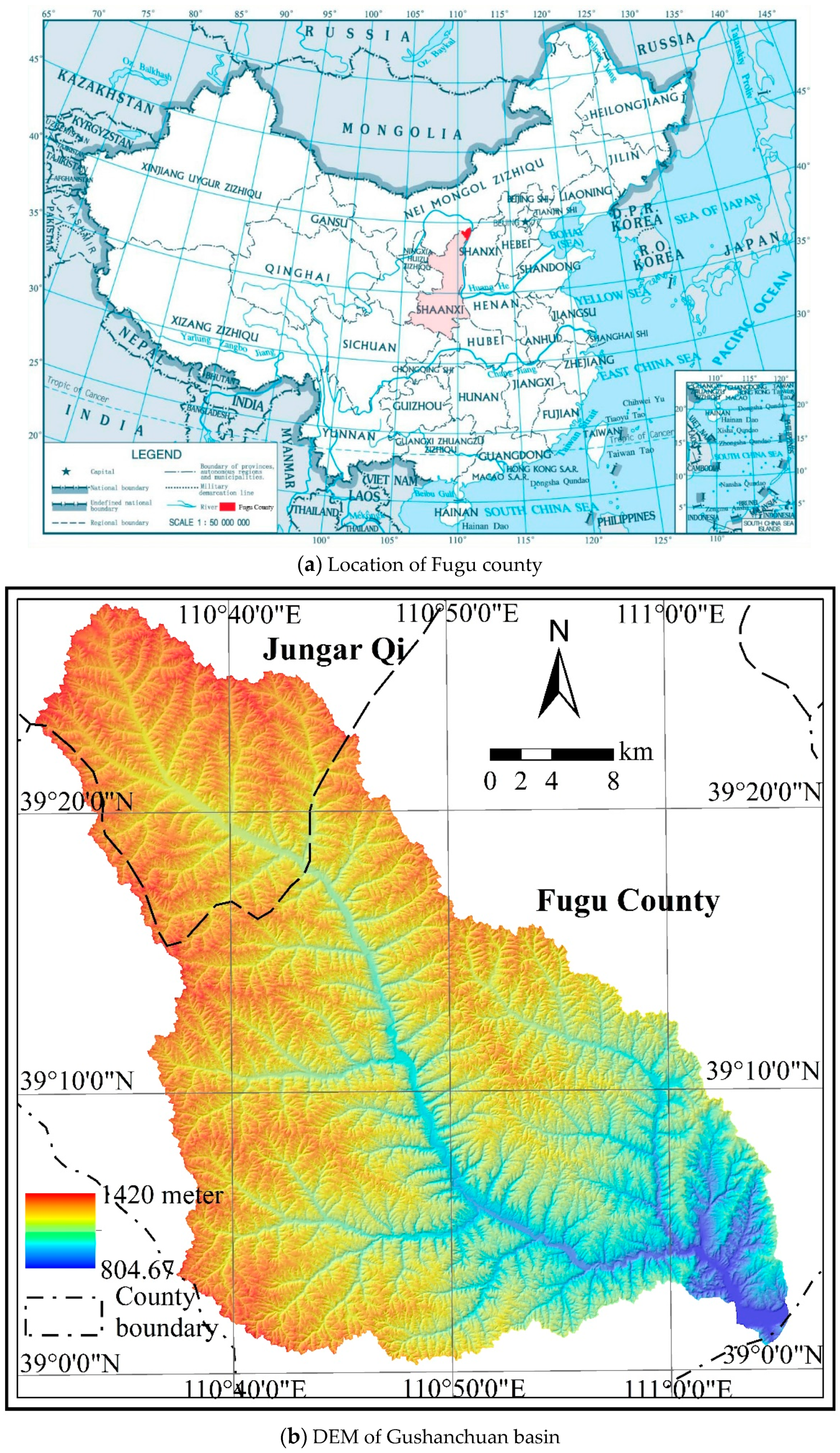
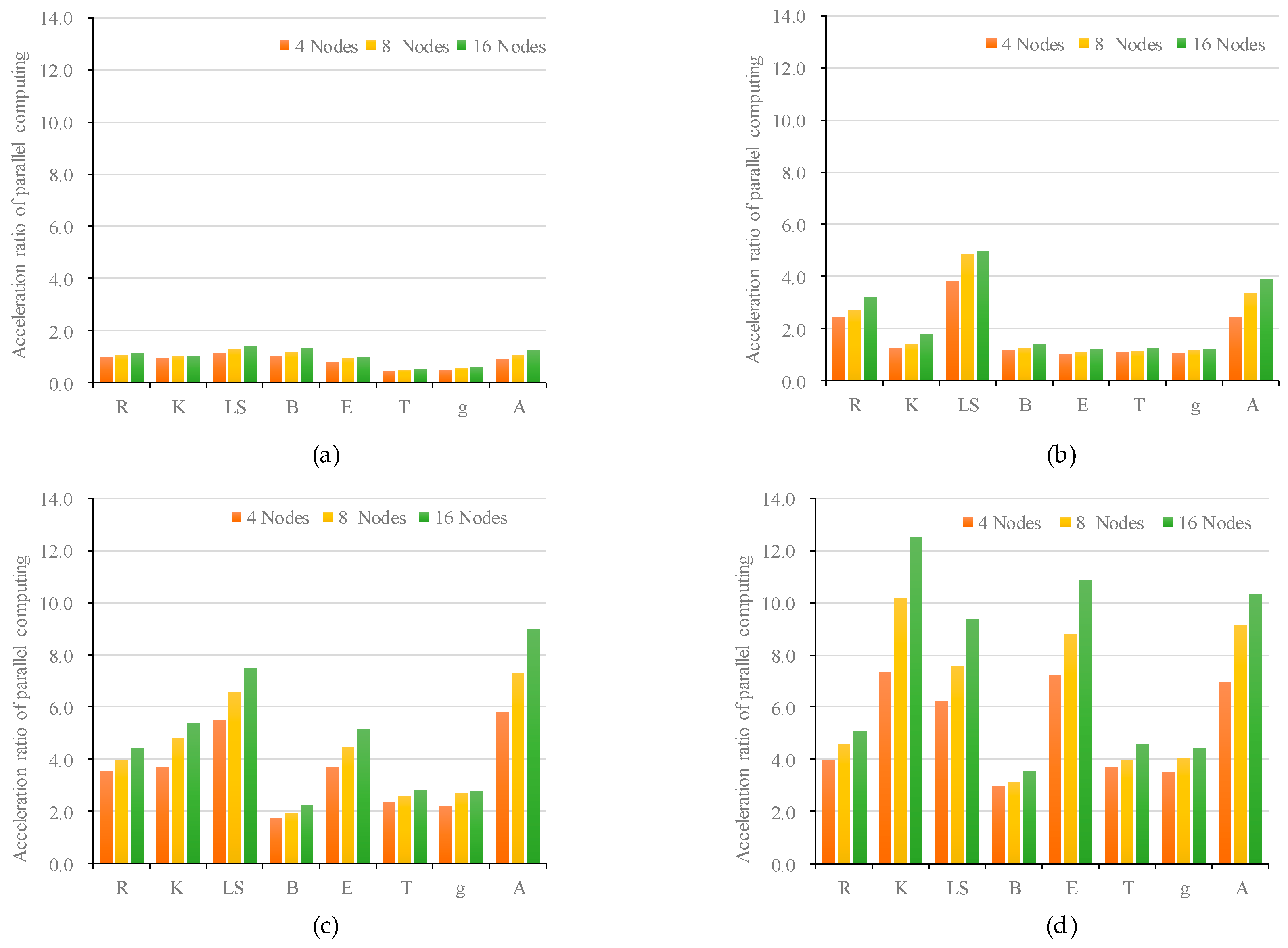
With the continuous development of geographic information acquisition technology, the requirements for soil erosion modelling and calculations have increased due to the broader availability of high-resolution data. Based on the Hadoop platform, an empirical model of soil erosion for annual sediment yield is selected to implement the Mr4Soil parallel computing framework. For three types of computing tasks, including local, focal, and zonal operations, two types of data-splitting strategies (row-based and sub-basin-based) are designed. Six parallel operators are defined, including spatial interpolation, vector rasterization, map algebra, slope gradient, flow direction, and slope length operators. The corresponding parallel algorithm is designed. A geoprocessing toolbox for model calculations is developed using the Python language based on the ArcGIS platform. The performance of the framework is analysed by taking the Gushanchuan basin on the Loess Plateau, China, as an example. With increases in the data resolution and volume, the computational efficiency of different model factors significantly improves, and a higher parallel acceleration ratio is achieved. The main contributions of this paper are as follows: (1) two data-splitting methods, row-based and sub-basin-based methods, and six parallel operators for local, focal and zonal soil erosion modelling computing tasks are developed; (2) a complete parallel computing framework for soil erosion modelling based on Hadoop platform is proposed; (3) a geoprocessing toolbox that integrates the parallel computing for soil erosion modelling with the GIS platform is constructed.

After analysing the performance of the implementation of the Mr4Soil, we found that, compared to parallel computing frameworks such as MPI, GPU, and UDA, the advantages of the proposed Mr4Soil framework are as follows: first, the Mr4Soil framework does not require specialized hardware, such as GPUs, and can achieve a high computational efficiency for a large-scale basin with high-resolution data. Moreover, the framework can be directly implemented on mainstream cloud computing platforms and has high scalability and usability. Second, the Mr4Soil framework was integrated with a GIS platform using a geoprocessing toolbox. It is easy to use for GIS users and provides essential support for using high-precision data to refine soil erosion modelling. Third, the Mr4Soil framework focuses on the parallel computing of soil erosion modelling, which is fully functional for different computing tasks and model factors.

For the parallel algorithm and geoprocessing toolbox development of the integration of GIS and soil erosion modelling parallel computing, this paper only describes a situation in which the GIS platform on a desktop and spatially distributed model are used. Further studies of the following two topics should be performed: (1) the creation of a service interface for the soil erosion model with parallel computing tasks, which could be based on a web service and conveniently applied in practice; and (2) the development of a physically based soil erosion model with parallel computing based on the Hadoop platform. These findings could extend parallel modelling studies of soil erosion.

References

1. Wischmeier, W.H.; Smith, D.D. Predicting Rainfall Erosion Losses—A Guide to Conservation Planning; United States Department of Agriculture: Hyattsville, MD, USA, 1978; pp. 1–58.
2. Kenneth, G.R.; George, R.F.; Weesies, G.A.; McCool, D.K.; Yoder, D.C. Predicting Soil Erosion By Water: A Guide to Conservation Planning with the Revised Universal Soil Loss Equation (RUSLE); United States Department of Agriculture: Washington, DC, USA, 1997; pp. 19–38.
3. Liu, B.; Zhang, K.; Xie, Y. An empirical soil loss equation. In Proceedings of the 12th International Soil Conservation Conference, Beijing, China, 26–31 May 2002; pp. 21–25. [Google Scholar]
4. Liu, B.; Bi, X.; Fu, S. Soil Erosion Equation in Beijing; Science Press: Beijing, China, 2010; pp. 36–66. [Google Scholar]
5. Joris, V.; Jean, P.; Gert, V.; Anton, V.R.; Gerard, G. Spatially distributed modelling of soil erosion and sediment yield at regional scales in Spain. Glob. Planet. Chang. 2008, 60, 393–415. [Google Scholar] [Green Version]
6. Ramsankaran, R.; Umesh, C.K.; Sanjay, K.G.; Andreas, M.; Krishnan, M. Physically-based distributed soil erosion and sediment yield model (DREAM) for simulating individual storm events. Hydrol. Sci. J. 2013, 58, 872–891. [Google Scholar] [CrossRef] [Green Version]
7. Dennis, C.F.; John, E.G.; Thomas, G.F. Water Erosion Prediction Project (WEPP): Development history, model capabilities, and future enhancements. Trans. ASABE 2007, 50, 1603–1612. [Google Scholar]
8. Jin, H.; Dennis, J.; Piyush, M.; Rupak, B.; Huang, L.; Barbara, C. High performance computing using MPI and OpenMP on multi-core parallel systems. Parallel Comput. 2011, 37, 562–575. [Google Scholar] [CrossRef] [Green Version]
9. Craig, A.L.; Samuel, D.G.; Antonio, P.; Chein-I, C.; Bormin, H. Recent developments in high performance computing for remote sensing: A review. IEEE J. Sel. Top. Appl. Earth Obs. Remote Sens. 2011, 4, 508–527. [Google Scholar]
10. Guan, Q.; Zeng, W.; Gong, J.; Yun, S. pRPL 2.0: Improving the parallel raster processing library. Trans. GIS 2014, 18, 25–52. [Google Scholar] [CrossRef]
11. Miao, J.; Guan, Q.; Hu, S. pRPL+ pGTIOL: The marriage of a parallel processing library and a parallel I/O library for big raster data. Environ. Model. Softw. 2017, 96, 347–360. [Google Scholar] [CrossRef]
12. Qin, C.; Zhan, L.; Zhu, A.; Zhou, C. A strategy for raster-based geocomputation under different parallel computing platforms. Int. J. Geogr. Inf. Sci. 2014, 28, 2127–2144. [Google Scholar] [CrossRef]
13. Zhang, J.; You, S. High-performance quadtree constructions on large-scale geospatial rasters using GPGPU parallel primitives. Int. J. Geogr. Inf. Sci. 2013, 27, 2207–2226. [Google Scholar] [CrossRef]
14. Jeffrey, D.; Sanjay, G. MapReduce: A flexible data processing tool. Commun. ACM 2010, 53, 72–77. [Google Scholar]
15. Deepak, V. Practical Hadoop Ecosystem: A Definitive Guide to Hadoop-Related Frameworks and Tools; Apress: New York, NY, USA, 2016; pp. 1–32. [Google Scholar]
16. Sam, R.A. Expert Hadoop Administration: Managing, Tuning, and Securing Spark, YARN, and HDFS; Addison-Wesley Professional: New York, NY, USA, 2016; pp. 4–18. [Google Scholar]
17. Ablimit, A.; Wang, F.; Vo, H.; Lee, R.; Liu, Q.; Zhang, X.; Joel, S. Hadoop GIS: A high performance spatial data warehousing system over mapreduce. Proc. VLDB Endow. 2013, 6, 1009–1020. [Google Scholar]
18. Ahmed, E.; Mohamed, F.M. Spatialhadoop: A mapreduce framework for spatial data. In Proceedings of the IEEE 31st International Conference on Data Engineering (ICDE), Seoul, Korea, 13–17 April 2015; pp. 1–12. [Google Scholar]
19. Louai, A.; Mohamed, F.M.; Mashaal, M. ST-HADOOP: A mapreduce framework for spatio-temporal data. GeoInformatica 2018, 22, 785–813. [Google Scholar]
20. Yu, J.; Zhang, Z.; Mohamed, S. Spatial data management in apache spark: The GeoSpark perspective and beyond. GeoInformatica 2018. [Google Scholar] [CrossRef]
21. Brian, L. Geoprocessing in the Cloud. Available online: http://gsaw.org/wp-content/uploads/2014/10/2010s11d_levy.pdf (accessed on 20 August 2018).
22. Jason, L. GIS Tools for Hadoop: Big Data Spatial Analytics for the Hadoop Framework. Available online: http://esri.github.io/gis-tools-for-hadoop (accessed on 20 August 2018).
23. Ameet, K.; Rob, E. Geotrellis: Adding Geospatial Capabilities to Spark. Available online: https://databricks.com/session/geotrellis-adding-geospatial-capabilities-to-spark (accessed on 20 August 2018).
24. Li, Z.; Hu, F.; John, L.S.; Daniel, Q.D.; Tsengdar, L.; Michael, K.B.; Yang, C. A spatiotemporal indexing approach for efficient processing of big array-based climate data with MapReduce. Int. J. Geogr. Inf. Sci. 2017, 31, 17–35. [Google Scholar] [CrossRef]
25. Li, Z.; Huang, Q.; Gregory, J.C.; Hu, F. A high performance query analytical framework for supporting data-intensive climate studies. Comput. Environ. Urban. Syst. 2017, 62, 210–221. [Google Scholar] [CrossRef]
26. Gao, S.; Li, L.; Li, W.; Janowicz, K.; Zhang, Y. Constructing gazetteers from volunteered big geo-data based on Hadoop. Comput. Environ. Urban. Syst. 2017, 61, 172–186. [Google Scholar] [CrossRef]
27. Li, W.; Shao, H.; Wang, S.; Zhou, X.; Wu, S. A2CI: A cloud-based, service-oriented geospatial cyberinfrastructure to support atmospheric research. In Cloud Computing in Ocean and Atmospheric Sciences; Tiffany, C.V., Nazila, M., Yang, C., Yuan, M., Eds.; Elsevier: London, UK, 2016; pp. 137–161. [Google Scholar]
28. Li, Z.; Michael, E.H.; Li, W. A general-purpose framework for parallel processing of large-scale LiDAR data. Int. J. Digit. Earth 2018, 11, 26–47. [Google Scholar] [CrossRef]
29. Muhammad, U.R.; Anand, P.; Awais, A.; Chen, B.; Huang, B.; Ji, W. Real-time big data analytical architecture for remote sensing application. IEEE J. Sel. Top. Appl. Earth Obs. Remote Sens. 2015, 8, 4610–4621. [Google Scholar]
30. Sara, M.; Damiano, C.; Alberto, B. Adaptive Trip Recommendation System: Balancing Travelers among POIs with MapReduce. In Proceedings of the IEEE International Congress on Big Data, San Francisco, CA, USA, 2–7 July 2018; pp. 1–5. [Google Scholar]
31. Deepak, P.; Surya, N.; Rajiv, R.; Chen, J. A secure big data stream analytics framework for disaster management on the cloud. In Proceedings of the 18th IEEE International Conference on High Performance Computing and Communications, Sydney, Australia, 12–14 December 2016; pp. 1218–1225. [Google Scholar]
32. Addair, T.G.; Douglas, A.D.; Walter, W.R.; Stan, D.R. Large-scale seismic signal analysis with Hadoop. Comput. Geosci. 2014, 66, 145–154. [Google Scholar] [CrossRef] [Green Version]
33. Yellow River Institute of Hydraulic Research. The Empirical Model of Annual Erosion and Sediment Production in Mesoscale Basins in Loess Plateau; Yellow River Institute of Hydraulic Research: Zhengzhou, China, 2013; pp. 26–56.
34. Tom, W. Hadoop: The Definitive Guide, 4th ed.; O’Reilly Media: Sebastopol, CA, USA, 2015; pp. 19–41. [Google Scholar]
35. Mahmoud, P. Data Algorithms: Recipes for Scaling Up with Hadoop and Spark; O’Reilly Media: Sebastopol, CA, USA, 2015; pp. 39–58. [Google Scholar]
Figure 1. Overview of parallel computing tools for the soil erosion model.
Ijgi 08 00103 g001
Figure 2. Data non-overlap splitting by row with 4 calculation nodes.
Ijgi 08 00103 g002
Figure 3. Data overlap splitting by row with 4 calculation nodes.
Ijgi 08 00103 g003
Figure 4. Data splitting by sub-basin with 4 calculation nodes.
Ijgi 08 00103 g004
Figure 5. Parallel algorithm example for spatial interpolation.
Ijgi 08 00103 g005
Figure 6. R Factor using row splitting based parallel algorithm.
Ijgi 08 00103 g006
Figure 7. Diagram of parallel algorithm for slope length.
Ijgi 08 00103 g007
Figure 8. LS factor using sub-basin splitting based parallel algorithm.
Ijgi 08 00103 g008
Figure 9. The calculation pipeline of the framework: connection with master node by SSHClient and SFTPClient in and ; uploading the input data to master node in and Hadoop HDFS in ; the model calculation in , and the output data download to master node in and local machine in from HDFS.
Ijgi 08 00103 g009
Figure 10. Mr4Soil toolbox and three tools.
Ijgi 08 00103 g010
Figure 11. Location and digital elevation model (DEM) of Gushanchuan basin.
Ijgi 08 00103 g011
Figure 12. Parallel acceleration ratio for data with different spatial resolution. (a) raster cell width with 30 m; (b) raster cell width with 10 m; (c) raster cell width with 5 m; (d) raster cell width with 2.5 m.
Ijgi 08 00103 g012
Figure 13. Time-consumption with different calculation tasks. (a) R factor; (b) K factor; (c) LS factor; (d) B factor; (e) E factor; (f) T factor; (g) g factor; (h) model A.
Ijgi 08 00103 g013
Figure 14. Time-consumption for slope calculation with graphics processing unit (GPU), central processing unit (CPU), unified device architecture (UDA), and different cluster size.
Ijgi 08 00103 g014