Abstract
Predicting the exact urban places where crime is most likely to occur is one of the greatest interests for Police Departments. Therefore, the goal of the research presented in this paper is to identify specific urban areas where a crime could happen in Manhattan, NY for every hour of a day. The outputs from this research are the following: (i) predicted land uses that generates the top three most committed crimes in Manhattan, by using machine learning (random forest and logistic regression), (ii) identifying the exact hours when most of the assaults are committed, together with hot spots during these hours, by applying time series and hot spot analysis, (iii) built hourly prediction models for assaults based on the land use, by deploying logistic regression. Assault, as a physical attack on someone, according to criminal law, is identified as the third most committed crime in Manhattan. Land use (residential, commercial, recreational, mixed use etc.) is assigned to every area or lot in Manhattan, determining the actual use or activities within each particular lot. While plotting assaults on the map for every hour, this investigation has identified that the hot spots where assaults occur were ‘moving’ and not confined to specific lots within Manhattan. This raises a number of questions: Why are hot spots of assaults not static in an urban environment? What makes them ‘move’—is it a particular urban pattern? Is the ‘movement’ of hot spots related to human activities during the day and night? Answering these questions helps to build the initial frame for assault prediction within every hour of a day. Knowing a specific land use vulnerability to assault during each exact hour can assist the police departments to allocate forces during those hours in risky areas. For the analysis, the study is using two datasets: a crime dataset with geographical locations of crime, date and time, and a geographic dataset about land uses with land use codes for every lot, each obtained from open databases. The study joins two datasets based on the spatial location and classifies data into 24 classes, based on the time range when the assault occurred. Machine learning methods reveal the effect of land uses on larceny, harassment and assault, the three most committed crimes in Manhattan. Finally, logistic regression provides hourly prediction models and unveils the type of land use where assaults could occur during each hour for both day and night.
1. Introduction
Crime is a social issue, like a disease, which tends to spread as geospatial clusters. Being of a geospatial character, crime has often been analyzed in terms of hot spots, spatial clusters, spatial correlations of different features with crime and predictions. Predicting where and when a crime can happen, also known as predictive policing, allows a city to deploy law enforcement to potentially dangerous areas or situations before a crime happens. Predictive policing deploys several programs, which have been created by scientists from different universities together with police departments and used in multiple cities. For instance, the PredPol program created by scientists of the University of California, Los Angeles (UCLA) and the Los Angeles Police Department identifies areas (or hot spots) where serious crimes are more likely to occur during a particular period: day or night for any of the requested days [1]. PredPol uses only three variables to predict where a crime could happen during each day: crime type, crime location and crime date/time. No personal identifiable information is ever used. No demographic, ethnic or socio-economic information is used. Predictions are displayed on an interactive map as red boxes that highlight the highest-risk areas [2]. Another example of crime-predicting software is CrimeScan, developed by scientists from Carnegie Mellon University and uses historical data about crimes and 911 calls about shots fired or a person seen with a weapon [3]. The program takes into account seasons and days of the week, as well as short-term and long-term rates of serious violent crimes [1]. For crime prediction and prevention, IBM uses structured data about crime along with unstructured data that includes incident reports, surveillance, sensor and social media data to not only monitor, measure and reduce crime, but to optimize resources, improve situational awareness by delivering information to the field where and when it is needed, and improve budgeting and planning by knowing what is likely to happen tomorrow, next week or next month [4]. The police department in Manchester, New Hampshire has used these IBM’s technologies to successfully reduce robbery rates by 28%. Chicago city took the next step by predicting people who are more likely to get involved in future shootings, either as a shooter or a victim. Their developed Strategic Subject List uses publicly available data and a linear regression model to make predictions about a person who could be involved in a possible upcoming shooting [5,6]. UK police have been using similar predictive policing software programs for a decade, where crime type, time and location are taken as input data, and a predicted hot spot of crime is generated as an output. Usually, historical data about committed crimes become the basis for these and similar programs. In addition, publicly available data is used in most of these cases. Israel, being a country with a high rate of terrorism, has developed a software program that is using streaming data from CCTV cameras on the streets to identify behavioral anomalies that could be an alarm that someone is about to commit a crime. In this case, developers are using the cortical segment of a rat’s brain instead of the neural networks, which allows developers to trace the error back and fix it without re-training the whole model, unlike what occurs in the deep learning process [7].
The variety of statistical methods and machine learning algorithms used for crime prediction depends on the problem to be solved, data (distribution, multicollinearity, noise etc.), and expected output (regression, classification, causality of crime etc.). Alves et al. [8] use random forest regression to predict crime and to quantify the influence of urban indicators on homicides. Their prediction model achieves 97% accuracy, and reveals unemployment and illiteracy as being the most important variables for describing homicides in Brazilian cities. While predicting whether a specific area in the city of London will be a crime hotspot or not, Bogomolov et al. [9] achieved the best accuracy (70%) when using a decision tree classifier based on the Breiman’s random forest on mobile phone and demographic data. Liu & Brown [10] used a point-pattern-based transition density model to predict criminal incidents based on historical crime data. Barreras et al. [11] explores four different methods for predicting crime hot spots in Bogota, Colombia, using historical crime data of 2011–2012: a point model, spatial ellipses model, spatio-temporal model and kernel density model. The later model achieved the best accuracy of an average metric over 20 different test weeks of data. Kianmehr and Alhajj [12] employ support vector machines (SVM) to predict crime hot spots. Liao et al. [13] are using the Bayesian learning theory on geographic data to predict the neighbourhood for the next crime in Gansu, China. Antolos et al. [14] use a logistic regression model to investigate the relationship between several predicting factors and burglary occurrence probability with regard to the epicenter, based on the day of the week, time of the day, repeated victimization, connectors and barriers, id est. and historical crime data from 2010. Zhu and Zhang [15] are using a statistical approach (probabilities of every point becoming a potential crime anchor point, multivariate analysis method to define the Euclidean and Manhattan distances between the anchor point and the locations of the previous crime sites, then according to distribution features of these distances they select the corresponding distribution function, finally, a fuzzy mathematical method gives quantified and normalized index factors, and an analytic hierarchy process computes different weights of social index factors of different areas in the region) to predict the potential locations of the next crime based on the time and locations of the previous crimes. The agent-based modelling method is used by a number of researchers to detect crime hot spots and spatial patterns of crime [16,17,18,19].
Several research cases have proven that planning of land use contributes to the decrease of crime. The research conducted by Stankevice et al. [20] demonstrates that specialized areas, greenery when included into dense residential areas, as well as public lands combined with residential and green areas, contribute to less crime. Another example is that pickpocketing often happens in mixed land use areas, mostly commercial. According to Newman [21], spaces with low urban development density and single use with strictly limited access to strangers are less vulnerable to crime, while Jacobs’s [22] opinion is opposite: urban spaces with mixed land use and open access to strangers lead to less crime because they provide more ‘eyes on the street’ and more natural surveillance. Hillier [23] and Monteiro [24] unveiled through their research that some types of anti-social behaviour happen only in areas of particular land uses. Additionally, Hiller [23] states that land use of urban areas, as well as low activity and movement are somehow related to crime. Sypion-Dutkowska and Leitner [25] discovered that the strong influence of land use types is limited to their immediate surroundings (i.e., within a distance of 50 meters), with commercial crimes and property theft showing the highest concentration compared to other types of crime. According to the results of their research on 31,319 crime events recorded by the police in 2006–2010 in the Polish city of Szczecin, alcohol outlets, clubs and discos, cultural facilities, municipal housing and commercial buildings are land use types that strongly attract crime. On the other hand, grandstands, cemeteries, green areas, allotment gardens, depots and transport bases strongly detract crime. Well-maintained urban spaces contribute to less crime, while abandoned areas do not attract people, therefore making them more vulnerable to crime.
This paper aims at predicting the effects of land uses on the top most committed crimes (larceny, harassment and assaults) in Manhattan, NY, and building hourly prediction models for assaults in Manhattan based on land uses of lots. The idea of analysing hourly assaults is related to the human activities within a day, as well as the police needs of knowing when and where an assault might happen. The research is based on the methods of geo-spatial data analysis, including hot spot and time series analysis, along with a descriptive analysis and data classification methods—logistic regression, k-nearest neighbors, Naïve Bayes, and random forest. While performing this research, it has been identified that hot spots of crime are ‘moving’ to different locations. This fact raises several questions. Why are hot spots of crime not static in an urban environment? What makes them—is it a specific urban pattern? Is the ‘movement’ of hot spots related to human activities during the day and night? Answering these questions help to predict the effect of land uses on the most committed crimes and to build the initial frame for assault prediction within every hour of a day. Knowing a specific land use vulnerability to where an assault could happen during an exact hour can assist police in allocating forces during those hours in risky areas.
2. Materials and Methods
The research is performed in Manhattan, NY, and lots with various land uses are the particular research objects. Land use is a common term in urban planning and official documents. Land use describes the current or planned human activities in a lot, for instance, one & two family buildings, parking facilities, etc. To analyze crimes through land use requires the combining of two datasets: data about crimes from NYC Open Data ‘NYPD Complaint Map’ (csv file) [26] and NYC Open Data about land uses within all lots in Manhattan, NY ‘Primary Land Use Tax Lot Output (PLUTO)’ (shp file) [27].
The dataset about land uses contains a unique ID, land use code and title (such as ‘One & Two Family Buildings’, ‘Multi-Family Walk-Up Buildings’, etc.), lot shape, area, tax code, address, as well as many other variables for each lot. The total number of variables is 84 in this dataset. It is geo-spatial data—each lot can be mapped as a polygon, having information for all 84 variables. Although, for this research the interest is only in the geo-spatial and land use information for all lots in Manhattan. Therefore, the dataset was mapped using ArcMap software and the number of variables were reduced; leaving the following variables for further research: unique ID, land use and geo-spatial attributes. Each land use is coded into a number, for instance 01—one & two family buildings, 02—multi-family walk-up buildings, etc. These codes of land use are used for the functional zoning and master plans of cities. Finally, the reduced dataset contains the following variables with their respective values (Table 1):

Table 1.
Geo-spatial dataset about land use.
The dataset about crimes contains geographical data for each crime (latitude and longitude) with crime type, date and time of when a crime was committed and registered by an officer of the police department, circumstances of crime, address, description of premises, and other variables. The total number of variables is 25 in this dataset. In addition, the granularity of crime classification into multiple crime sub-types presented in this dataset is very small for this research, for instance, assault is classified as assault 1, assault 2, assault peace officer, etc. As the very small granularity of crimes is out of the research goal, and the research does not focus on the smaller sub-types of crime (for instance, larceny in chain stores, larceny in boutiques, larceny in clothing stores, etc.), this paper has aggregated crime sub-types into larger groups, such as larceny, harassment, assault, burglary, etc., using only crime data for 2015–2017. In crime analysis, especially crime in terms of urban planning, data from the recent two-three years is the most commonly used.
In this research the paper focuses on the top three most committed crimes in Manhattan (larceny, harassment and assaults) for predicting the effect of land use in these crimes. Then the paper presents assaults in more detail, while building hourly prediction models for assaults based on land use. The primary data analysis of the whole dataset about crime for 2015–2017 has revealed that larceny was the largest crime in Manhattan with 41,836 registered cases by police, resulting in 36.22% of all crimes. Larceny is followed by harassment, having 13,245 registered cases, resulting in 11.46% of all crimes. Assault was the third largest crime in Manhattan (after larceny and harassment) with 12,244 registered cases, resulting in 10.6% of all crimes. According to the criminal law and the Penal Code, larceny is ‘the unlawful taking and carrying away of someone else’s property without the consent of the owner and with the intent to permanently deprive the owner of the property’ [28]. Criminal harassment entails ‘intentionally targeting someone else with behavior that is meant to alarm, annoy, torment or terrorize them’ [28], although, states in the USA vary in how they define criminal harassment. In criminal law, assault is ‘a physical attack on someone’. Under New York Penal Law, assault is when a person i) has an intent to cause physical injury to another person, or ii) he recklessly causes physical injury to another person, or iii) with criminal negligence, he causes physical injury to another person by means of a deadly weapon or a dangerous instrument [28].
Further to this, using R programming language the investigation has performed a dimensionality reduction in the dataset about crime, extracting for each crime only the variables that are required in further research: crime type (larceny, harassment and assault), latitude, longitude, date, and time. Finally, the reduced dataset contains the following variables with the respective values (Table 2):
Table 2.
Dataset about crimes, after the dimensionality reduction (extract).
To proceed with the data analysis, both datasets (crime and land use) need to be joined, although, they do not have any common key value to join them. Therefore, joining by a location method is applied to the datasets containing geo-spatial data. Joining by location, or spatial join, uses spatial associations between the layers involved to append fields from one layer to another. Spatial joins are different from attribute and relationship class joins, because they are not dynamic and require the results to be saved to a new output layer. Therefore, ArcGIS was used for joining the two datasets. Firstly, csv and shp files are imported into ArcMap. For the csv file (dataset about assaults) the table with data is geo-located in XY coordinates. Although, data mapped in this way does not have a unique ID (key) to proceed with data processing. Therefore, the created layer file with XY coordinates is converted into a shp file and imported into ArcMap. Secondly, the dataset about crimes (now the shp file!) is joined to the ‘Land use’ dataset based on spatial location of the ‘Land use’ dataset (which is a layer). Thus, each lot is assigned properties of the joined layer (dataset about crimes), where each polygon (a lot) is given attributes of the point (crime) that is closest to its boundary, or falling inside a polygon. Therefore, the final dataset is geo-spatial data, where each lot carries information about its land use and crimes occurred within a polygon (Table 3). The final dataset has 42,687 instances (rows).
Table 3.
Final geo-spatial dataset (extract).
For predicting the effects of land uses on larceny, harassment and assaults, research uses machine learning methods—logistic regression, k-nearest neighbors, Naïve Bayes and random forest. 75/25 data split into the training and test sets is used for this task. Each of the algorithms train the prediction model on the training set (randomly chosen 75% of instances in the final dataset) and then predicts the y-values (1–0 as a crime will happen or not) using the test set (the rest 25% of instances in the dataset). Accuracy metric is used to check the performance of the above described methods. Accuracy (ranging from 0 to 1) is computed as the number of correctly classified cases divided by the total number of all cases. The closer the accuracy to 1, the better the performance of the prediction model. Therefore, based on the best performing machine learning method, the land uses effecting a particular crime are extracted for each crime type.
For a more detailed investigation and building hourly prediction models, research uses data about assaults and land uses. First, it uses hot spot analysis and time series analysis for the initial data investigation. For the hot spot analysis, the statistic is computed for assaults within each hour of a day and night, using the formulas (1) integrated in the ArcGIS software. The computed statistic is a z-score that indicates where assaults with either high or low values cluster spatially. For statistically significant positive z-scores, the larger the z-score is, the more intense the clustering of high values (hot spot). For statistically significant negative z-scores, the smaller the z-score is, the more intense the clustering of low values (cold spot). A statistically significant hot spot is based on a variable having a high value and surrounded by other features with high values as well. The computed sum for a variable and its neighbours is compared proportionally to the sum of all variables. This indicates a statistically significant z-score when the sum differs a lot from the expected sum, and when that difference is too large to be the result of random chance [29,30,31,32]. Also, hot spot analysis using the ArcGIS software computes p-values and confidence level bins (Gi_Bin) for assaults. Further, for the correlation analysis and building hourly prediction models, the data is converted into binary in the following way: assault data is coded as 1 if an assault is committed in the analysed lot, and 0 if no assault is committed. Then, the assaults data is divided into 24 classes based on the time when the assault occurred, for instance, between 0–1 a.m. class, between 1–2 a.m. class, etc. Data about land uses is presented as dummy variables in the following way: for instance, for the land use variable ‘One & two family buildings’—the data is coded as 1 if the land use code is 01 (id est. one & two family buildings), and coded 0 if the land use code is different. In the same way, the data coding for land uses 02, 03, 04, 05, 06, 07, 08, 09, 10, 11 is identified. The model uses R programming language for the coding, as well as for building hourly prediction models. Using the machine learning prediction model, which has the best performance metric (accuracy), for every class of time range shows the probability of an assault to happen during a particular hour, and reveals land uses that generate assault during the analysed hour. Using the logistic regression requires the model to meet the following assumptions: (i) the dependent variable has to be binary or ordinal, (ii) observations must be independent of each other, id est. should not come from repeated measurements or matched data, (iii) there should be little or no multicollinearity among the independent variables, (iv) a sample size has to be large. Regarding multicollinearity, it is important to avoid any two independent variables that are highly correlated, because they cause a multicollinearity problem in the regression model. Therefore, correlation analysis is performed by using the Pearson correlation coefficient (describes relation between variables in terms of linearity—assault and land use) and Kendall correlation coefficient (describes association between two quantities—assault and land use). To build the logistic regression model, the Backward selection was used (starting with the full model and dropping one variable at a time that has the largest p-value).
Geti-Ord local statistic formula. Here xj is the attribute value for feature j, wi,j is the spatial weight between features i and j, and n is the total number of features. statistic is a z-score.
3. Results
3.1. Predicting the Effects of Land Uses on Crime
To predict the effects of land uses on larceny, harassment and assaults regardless time ranges the research applies logistic regression, k-nearest neighbors, Naïve Bayes and random forest for each crime type. Also it compares (data classification) accuracy of each method (Table 4), and extracts land uses effecting that particular crime based on the best performing prediction model. The whole final dataset of 42,687 instances is used for this purpose. The best achieved accuracy is presented in bold for each crime in Table 4. It is obvious from Table 4 that logistic regression produces the best classification results for larceny and assault. Whereas, random forest achieves the best accuracy for the harassment data. Therefore, logistic regression is used to predict the effects of land uses on larceny and assault, and random forest is used to predict the effect of land uses on harassment.
Table 4.
Choosing the best performing prediction model based on accuracy.
Using the logistic regression output, the research has identified the following land uses that significantly (p-value < 0.05) effect larceny: LU3 (multi-family elevator buildings), LU4 (mixed residential & commercial buildings), LU5 (commercial & office buildings), LU8 (public facilities & institutions) and LU9 (open space and outdoor recreation). All these land uses, except LU9, have negative prediction estimates, meaning that larceny is not likely to be committed on lots with LU3, LU4, LU5 and LU8 land uses. Whereas, larceny is more likely to be committed on lots having LU9 land use.
Using the logistic regression output, the research has identified that LU9 (open space and outdoor recreation) land use significantly (p-value < 0.05) effects assault, having a positive prediction estimate. Therefore, assault is more likely to be committed on lots of LU9 land use. Since the whole dataset is used for this task, more and different land uses generating assault might be identified while using subsets of data based on twenty-four time ranges.
Similarly, the random forest method has identified LU9 (open space and outdoor recreation) land use effecting harassment.
3.2. Time Series and Hot Spot Analysis of Assaults
Assaults have been selected for a more detailed analysis, using time series and hot spot analysis of data. To see how the location and intensity of assaults varies within Manhattan, NY in a 24 h period of a day, the model has classified data into 24 classes based on the time when the assault occurred, for instance, 0–1 a.m. class, 1–2 a.m. class, etc. Time series analysis reveals trends in time classes for assaults. It can be identified that the least number of assaults happen at 7 a.m. (230 assaults) and the most at 11 p.m. (682 assaults) (Figure 1). It is also clear from Figure 1 that the number of assaults gradually increase from 7 a.m. to 11 p.m., with a decrease observed from 1 a.m. to 6 a.m. (Figure 1). This is explained by human activities during morning-day-evening hours, and night hours accordingly.
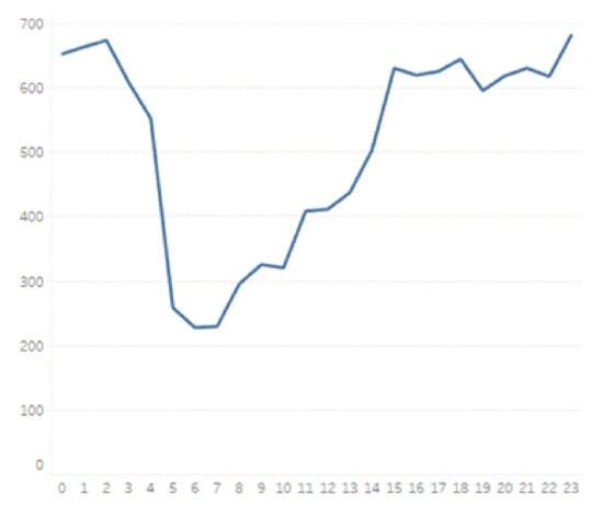
Figure 1.
Time series plot of assaults in Manhattan, NY. The number of assaults increases from 7 a.m. to 11 p.m. (where 11 p.m. is the peak of assaults), and decreases during night hours from 1 a.m. to 6 a.m.
Having performed the hot spot analysis for each class of 24 h. The hot spot analysis uses the locations and intensity of occurrence of geo-spatial data to compute and visualize hot spots. This analysis reveals that hot spots ‘move’ within Manhattan, depending on the time when the assault was committed (Figure 2). It is also obvious from Figure 2 that during day time assaults happen in a greater number of lots, though, they mostly form less statistically significant hot spots at 90% of confidence level (Figure 2). For instance, at 12 p.m. and 3 p.m. these are mostly single assaults per lot happening in a greater number of lots, compared to 11 p.m. where multiple assaults per lot occur and less lots are affected by an assault.
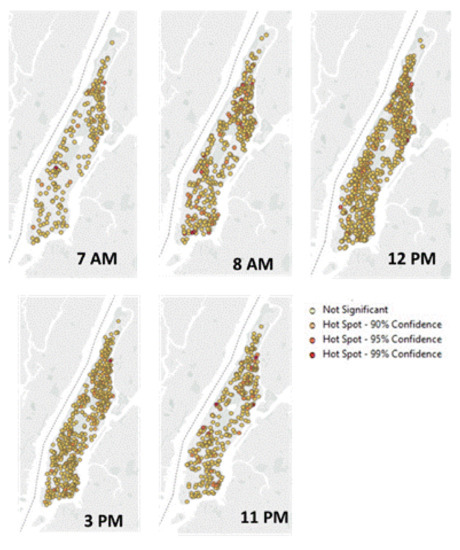
Figure 2.
Hot spots of assaults committed in Manhattan, NY. Location of assaults and their intensity demonstrate that hot spots “move” within Manhattan depending on the time when the assault was committed. At 7 a.m. there is one statistically significant hot spot (at a 99% confidence level) in Midtown and one in Uptown, whereas, at 11 p.m. (peak time for assaults) there are four statistically highly significant hot spots in Midtown, and a couple in both Uptown and Downtown Manhattan.
3.3. Hourly Prediction Models for Assaults
Based on the findings in Section 3.1, where research has identified logistic regression giving the best accuracy for prediction model, logistic regression is used further to build hourly prediction models for assaults. To build a good regression model, researchers checked the assumptions for the logistic regression. First, the independent variable Crime is binary; having a value of 0 for lots with no assault committed, and 1 for lots with at least one incident of assault. Second, the observations are independent and not coming from repeated measurements or matched data. Third, data is checked for missing values and multicollinearity. For the missing values—after it is identified that the character is missing values, researchers have excluded them from the analysis. After checking the variables for multicollinearity, the correlation analysis did not find any independent variables that are strongly related (r > 0.9). Therefore, the model has no multicollinearity problem in the data. Finally, a large enough sample size is acquired, with the total number of observations being 42,687.
To identify land uses, if any, that are related to the commitment of assault, researchers perform correlation analysis for all twenty four time classes using the Pearson correlation coefficient. The analysis results show the correlation coefficients varying between 0.03 and 0.85 (both negative and positive) between assault and various land uses for different time ranges. Therefore, there are linear relations between some land uses and assault.
Following this, to reveal when and how land use generates assault to be committed, researchers performed logistic regression analysis. Prediction models for assaults are computed for each time range out of twenty-four, with Table 5 demonstrating some of these models and their accuracy for eight time classes. In the table, the first column ‘Land Use’ demonstrates only those land uses that impact the occurrence of assault. For instance, LU1 means 01 code of land use (one & two family buildings), LU2 means 02 code of land use (multi-family walk-up buildings), etc. The column ‘Estimate’ means the coefficient of the log-odds of the independent variable (land use) in the regression model. The higher the estimate value the greater the probability of an assault to happen during the distinct hour. These estimates identify the amount of increase in the predicted log odds of Assault = 1 that would be predicted by the predictor = 1, holding all other predictors constant. For instance, having the coefficient (or parameter estimate) for the variable LU3 = 2.63 (Table 5) means that for a LU3 = 1 (id est. the land use of the lot is multi-family elevator buildings), we expect a 2.63 increase in the log-odds of the dependent variable Assault, holding all other independent variables constant. As an example: log-odds , and accordingly the probability of an Assault to happen is = = 0.93. P-value shows the significance of each independent variable. Prediction models only with all significant variables (p-value < 0.05) are considered as significant in this research and, therefore, presented in Table 5. Due to a large number of significant prediction models (22 models in total) in this paper, researchers present only 8 of them.
Table 5.
Prediction models for different time ranges.
Some interesting dependencies between land uses and assaults have been extracted from the logistic regression models for different time ranges:
- It is interesting that the probability of the logit of assault to occur during time ranges 2:00–2:59 a.m., 4:00–4:59 a.m., 5:00–5:59 a.m., 6:00–6:59 a.m., and 7:00–7:59 a.m. is predicted by the same land uses: LU1 one & two family buildings and LU2 multi-family walk-up buildings with all estimates in the prediction models being negative (Table 5). This means, for the time ranges 2:00–2:59 a.m., 4:00–4:59 a.m., 5:00–5:59 a.m., 6:00–6:59 a.m., and 7:00–7:59 a.m. land uses LU1 and LU2 contribute to the decrease of the probability of the logit of assault.
- Also, the probability of the logit of assault during time ranges 3:00–3:59 a.m., 8:00–8:59 a.m., and 7:00–7:59 p.m. is predicted by the same land use LU1 one & two family buildings, in all three prediction models for these time ranges the estimates are negative (Table 5), meaning that for the time ranges 3:00–3:59 a.m., 8:00–8:59 a.m., and 7:00–7:59 p.m. land use LU1 contributes to the decrease of the probability of the logit of assault.
- The probability of logit of assault during time ranges 1:00–1:59 a.m., 9:00–9:59 a.m., and 11:00–11:59 p.m. is predicted by the same land uses: LU1 one & two family buildings, LU2 multi-family walk-up buildings, and LU11 vacant land, with all estimates in the prediction models being negative (Table 5). This means, for the time ranges 1:00–1:59 a.m., 9:00–9:59 a.m., and 11:00–11:59 p.m. land uses LU1, LU2 and LU11 contribute to the decrease of the probability of the logit of assault.
- The probability of the logit of assault to occur during time ranges 2:00–2:59 p.m., 3:00–3:59 p.m., 9:00–9:59 p.m., and 10:00–10:59 p.m. is predicted by the following land uses: LU1 one & two family buildings, LU2 multi-family walk-up buildings, and LU9 open space and outdoor recreation, where LU1 and LU2 land uses have negative estimates in all four time ranges, and only LU9 land use has a positive estimate for all four time ranges (Table 5). This explains that for the time ranges 2:00–2:59 p.m., 3:00–3:59 p.m., 9:00–9:59 p.m., and 10:00–10:59 p.m. land uses LU1 and LU2 contribute to the decrease of the probability of the logit of assault, but the land use LU9 contributes to the increase of the probability of the logit of assault.
Researchers could not compute a proper prediction model for classes with a time range 10:00–10:59 a.m. and 8:00–8:59 p.m., because there are no significant relations. Though, with p-values < 0.05 in the rest of the 22 models, researchers concluded there is strong evidence against the H0 hypothesis that the land use has no effect on the occurrence of assault. Therefore, reject H0: r = 0, and state with 95% confidence that there is an effect of some land uses with p-values < 0.05 on the logit of assaults.
4. Discussion and Conclusions
This research demonstrates the following achieved results: (1) machine learning algorithms predict land uses effecting the most commonly committed crimes in Manhattan, NY—larceny, harassment and assault, (2) time series and hot spot analysis identify exact hours when most of assaults have been committed, as well as hot spots of assaults within different time ranges, (3) logistic regression model predicts land uses that generate assaults during different hours. Results and discussion are presented in more details below.
Using the whole dataset (without splitting into time ranges), machine learning methods reveal the following land uses generating crimes: LU9 (open space and outdoor recreation) generates larceny, harassment and assault, meaning that LU9 areas are the most unsafe in Manhattan, NY, in terms of the analyzed top three crimes. Whereas, on lots with land uses LU3 (multi-family elevator buildings), LU4 (mixed residential & commercial buildings), LU5 (commercial & office buildings), LU8 (public facilities & institutions) larceny might likely not to be committed. Open space and outdoor recreation, such as parks and green spaces, are often more vulnerable to crime because usually they are less observed during dark periods (less or no visitors) and have too many strangers at day time (regarding the Crime Prevention through Environmental Design CPTED strategies, presence of strangers in urban spaces make them less safe).
Research of assault in more detail (while splitting the data into twenty-four time ranges) and land use reveals some tendencies and unveils land uses that generate assault during some hours. Firstly, the time series plot demonstrates an increasing number of assaults from 7 a.m. to 11 p.m. with its peak in 11 p.m., and a decreasing number of assaults from 1 a.m. to 6 a.m. Human behaviour during these time ranges explains the shifting number of assaults: during the night hours, city dwellers sleep; and from morning until late evening they are active.
Secondly, mapping the data of assaults for each time class separately, and using the hot spot analysis demonstrate clearly that hot spots of assaults are ‘moving’ within Manhattan. Additionally, morning and especially day time classes demonstrate more lots affected by assault with mostly a single assault per lot, and therefore, less highly significant hot spots of assaults. Whereas, evening time classes demonstrate less lots affected by assault and therefore more hot spots where assaults concentrate in a higher intensity per lot.
Thirdly, using the logistic regression, researchers identify different land uses generating assault during different hours of a day or night. It was identified that during almost all hours the land use 01 one & two family buildings generates assaults. The second largest assault generator is land use 02 multi-family walk-up buildings, the third is land use 11 vacant land and land use 09 open space and outdoor recreation, such as parks. This means that assaults are most likely to occur in the areas with low-rise residential buildings (land use codes 01 and 02), as well as areas that have no obvious owner (land use codes 09 and 11), which are unmaintained and have no natural surveillance (land use code 11). The interesting discovery is that land use 08 public facilities & institutions does not generate any assault within any class of time range. According to the prediction models, land use 03 multi-family elevator buildings, land use 05 commercial & office buildings and land use 07 transportation & utility generate assaults only during the period 0:00–0:59 a.m., whereas, land use 04 mixed residential & commercial buildings and land use 10 parking facilities contribute to the occurrence of assaults only during the period 12:00–12:59 p.m. Since the logistic regression models meet all assumptions for a model to be valid, they are applicable for the whole of Manhattan to predict land uses generating crime. Though, to make a conclusion about another city, the model needs to be trained on the data from that city. Also, to update the prediction model, new data must be used.
This research, as well as other research in this field, aims to narrow down crime prediction to exact areas where the next crime could be committed. In the majority of other research, these areas are identified as hot spots, by applying statistical, machine learning and simulation methods. Differently from others, the research in this paper identifies land uses (not hot spots) responsible for crime generation. In addition, these land uses are identified for each hour (not for the whole data set without considering time of a committed crime), demonstrating that different human activities during different time periods could lead to a crime to be committed. In terms of land use and crime, Sypion-Dutkowska [25] applied geo-spatial statistical analysis methods and GIS tools. Differently from that, methods presented in this paper go a step further by using geo-spatial analysis methods as a basement for the further application of machine learning algorithms on merged geo-spatial data.
Although in the frames of this research the models did not identify exact places where an assault will occur during the expected hour, the results narrow the search field and direction to lots of defined land uses that generate assault during an exact hour. Using master plan and other urban development documents together with the research results would help police officers to foresee the next assault and to allocate their forces accordingly in risky areas within risky hours.
Despite multiple studies, the prediction of the exact place and time of a crime remains the unsolved problem for police and researchers. Therefore, to make research results more precise, the next steps in research are to try different groupings of crime data (different time range, time within months, aggregated groups by location instead of land use, etc.) and new methods (for instance, neural networks would allow to both classify data and to develop prediction models).
Police, Scientists, researchers and authors should discuss the results and how they can be interpreted in perspective of previous studies and of the working hypotheses. The findings and their implications should be discussed in the broadest context possible. Future research directions may therefore also be highlighted.
Author Contributions
Conceptualization, I.M.; methodology, I.M. and P.Z.; software, I.M. and P.Z.; validation, I.M.; formal analysis, I.M.; investigation, I.M.; resources, S.J. and J.W.G.J.; data curation, I.M.; writing—original draft preparation, I.M.; writing—review and editing, S.J.; visualization, I.M.; funding acquisition, J.W.G.J.
Funding
This research received no external funding.
Conflicts of Interest
The authors declare no conflict of interest.
References
- Rieland, R. Artificial Intelligence Is Now Used to Predict Crime. 2018. Available online: https://www.smithsonianmag.com/innovation/artificial-intelligence-is-now-used-predict-crime-is-it-biased-180968337/ (accessed on 30 July 2018).
- Predpol. How Predictive Policing Works. 2018. Available online: http://www.predpol.com/how-predictive-policing-works/ (accessed on 30 July 2018).
- Neill, D.B. Predicting and Preventing Emerging Outbreaks of Crime. 2012. Available online: https://www.cs.cmu.edu/~neill/papers/mlss2012.pdf (accessed on 30 July 2018).
- IBM. Crime Prediction and Prevention. 2018. Available online: https://www.ibm.com/industries/government/public-safety/crime-prediction-prevention (accessed on 30 July 2018).
- Asher, J.; Arthur, R. Inside the Algorithm that Tries to Predict Gun Violence in Chicago. 2017. Available online: https://www.nytimes.com/2017/06/13/upshot/what-an-algorithm-reveals-about-life-on-chicagos-high-risk-list.html (accessed on 30 July 2018).
- Chicago Data Portal. Strategic Subject List. 2017. Available online: https://data.cityofchicago.org/Public-Safety/Strategic-Subject-List/4aki-r3np (accessed on 30 July 2018).
- Cortica. Cortica Smart City. 2018. Available online: https://www.cortica.com/smartcity/index.html (accessed on 31 July 2018).
- Alves, L.G.A.; Ribeiro, H.V.; Rodrigues, F.A. Crime prediction through urban metrics and statistical learning. Phys. A Stat. Mech. Its Appl. 2018, 505, 435–443. [Google Scholar] [CrossRef]
- Bogomolov, A.; Lepri, B.; Staiano, J.; Oliver, N.; Pianesi, F.; Pentland, A. Once upon a crime: Towards crime prediction from demographics and mobile data. In Proceedings of the 16th International Conference on Multimodal Interaction, Istanbul, Turkey, 12–16 November 2014; pp. 427–434. [Google Scholar]
- Liu, H.; Brown, D.E. Criminal incident prediction using a point-pattern-based density model. Int. J. Forecast. 2003, 19, 603–622. [Google Scholar] [CrossRef]
- Barreras, F.; Diaz, C.; Riascos, A.; Ribero, M. Comparison of Different Crime Prediction Models in Bogotá. 2016. Available online: http://www.alvaroriascos.com/researchDocuments/PrediccionCrimen.pdf (accessed on 30 July 2018).
- Kianmehr, K.; Alhajj, R. Crime Hot-spots prediction using support vector machine. In Proceedings of the IEEE International Conference on Computer Systems and Applications, Dubai, UAE, 8 March 2006; pp. 952–959. [Google Scholar]
- Liao, R.; Wang, X.; Li, L.; Qinh, Z. A Novel Serial Crime Prediction Model Based on Bayesian Learning Theory. In Proceedings of the International Conference on Machine Learning and Cybernatics, Qingdao, China, 11–14 July 2013; pp. 1757–1762. [Google Scholar]
- Antolos, D.; Liu, D.; Ludu, A.; Vincenzi, D. Burglary Crime Analysis Using Logistic Regression. In Human Interface and the Management of Information. Information and Interaction for Learning Culture Collaboration and Business; Lecture Notes in Computer Science; Springer: Berlin/Heidelberg, Germany, 2013; Volume 8018, pp. 549–558. [Google Scholar]
- Zhu, K.; Zhang, J. Predicting the potential locations of the next crime based on data mining: A case study. Int. J. Digit. Content Technol. Its Appl. 2012, 6, 574–581. [Google Scholar]
- Malleson, N.; Heppenstall, A.; See, L.; Evans, A. Using an Agent-Based Crime Simulation to Predict the Effects of Urban Regeneration on Individual Household Burglary Risk. Environ. Plan. B Urban Anal. City Sci. 2013, 40, 405–426. [Google Scholar] [CrossRef]
- Malleson, N.; Heppenstall, A.; See, L. Crime reduction through simulation: An agent-based model of burglary. Comput. Environ. Urban Syst. 2010, 3, 236–250. [Google Scholar] [CrossRef]
- Peng, C.; Kurland, J. The Agent-Based Spatial Simulation to the Burglary in Beijing. In Computational Science and Its Applications—ICCSA 2014; Murgante, B., Misra, S., Rocha, A.M.A.C., Torre, C., Rocha, J.G., Falcão, M.I., Taniar, D., Apduhan, B.O., Gervasi, O., Eds.; Lecture Notes in Computer Science; Springer: Cham, Switzerland, 2014; Volume 8582, pp. 31–43. [Google Scholar]
- Roses, R.; Kadar, B.C.; Cvijikj, I.P. Design of an agent-based model to predict crime (WIP). In Proceedings of the Summer Computer Simulation Conference SCSC’16, Montreal, QC, Canada, 24–27 July 2016. [Google Scholar]
- Stankevice, I.; Sinkiene, J.; Zaleckis, K.; Matijosaitiene, I.; Navickaite, K. What does a city master plan tell us about our safety? Comparative analysis of Vilnius, Kaunas and Klaipeda. Soc. Sci. 2013, 2, 64–76. [Google Scholar]
- Newman, O. Defensible Space: Crime Prevention through Urban Design; DIANE Publishing: New York, NY, USA, 1972. [Google Scholar]
- Jacobs, J. The Death and Life of Great American Cities; Random House: New York, NY, USA, 1961. [Google Scholar]
- Hillier, B.; Sahbaz, O. Crime and urban design: An evidence-based approach. In Designing Sustainable Cities; Cooper, R., Evans, G., Boycko, C., Eds.; Wiley-Blackwell: Singapore, 2009; pp. 163–186. [Google Scholar]
- Monteiro, L.T. The Valley of Fear—The morphology of crime, a case study in João Pessoa, Paraíba, Brasil. In Proceedings: Eighth International Space Syntax Symposium; Greene, M., Reyes, J., Castro, A., Eds.; PUC: Santiago, Chile, 2012; pp. 3:01–3:17. [Google Scholar]
- Sypion-Dutkowska, N.; Leitner, M. Land use influencing the spatial distribution of urban crime. A case study of Szczecin, Poland. Int. J. Geo-Inf. 2017, 6, 74–97. [Google Scholar] [CrossRef]
- NYC Open Data. NYPD Complaint Map [Dataset]. 2016. Available online: https://data.cityofnewyork.us/Public-Safety/NYPD-Complaint-Map-Historic-/57mv-nv28/data (accessed on 1 February 2018).
- NYC Open Data. Primary Land Use Tax Lot Output (PLUTO) [Dataset]. 2013. Available online: https://data.cityofnewyork.us/City-Government/Primary-Land-Use-Tax-Lot-Output-PLUTO-/xuk2-nczf (accessed on 1 February 2018).
- New York Laws. PEN—Penal. Part 3—Specific Offences. Title H—Offences against the person involving physical injury, sexual conduct, restraint and intimidation. Article 120—Assault and Related Offences. 2015. Available online: https://law.justia.com/codes/new-york/2015/pen/part-3/title-h/article-120/120.10/ (accessed on 14 November 2018).
- Getis, A.; Ord, J.K. The Analysis of Spatial Association by Use of Distance Statistics. Geogr. Anal. 1992, 24, 189–206. [Google Scholar] [CrossRef]
- Mitchell, A. The ESRI Guide to GIS Analysis; ESRI Press: Redlands, CA, USA, 2005. [Google Scholar]
- Ord, J.K.; Getis, A. Local Spatial Autocorrelation Statistics: Distributional Issues and an Application. Geogr. Anal. 1995, 27, 286–306. [Google Scholar] [CrossRef]
- Scott, L.; Warmerdam, N. Extend Crime Analysis with ArcGIS Spatial Statistics Tools. Available online: https://www.esri.com/library/reprints/pdfs/arcuser_extend-crime-analysis.pdf (accessed on 30 July 2018).
© 2018 by the authors. Licensee MDPI, Basel, Switzerland. This article is an open access article distributed under the terms and conditions of the Creative Commons Attribution (CC BY) license (http://creativecommons.org/licenses/by/4.0/).