Spatial Assessment of the Potential Impact of Infrastructure Development on Biodiversity Conservation in Lowland Nepal

Abstract

Biodiversity is declining at an unprecedented rate with infrastructure development being one of the leading causes. New infrastructure, such as roads, provides new access and results in increased land clearing and wildlife hunting. A number of large infrastructure projects, including new roads and rail, are being planned in Nepal. We show the application of readily available remotely sensed data and geospatial tools to assess the potential impact of these future developments on habitat quality under three protection-level scenarios. Our findings reveal that there is currently large spatial heterogeneity in habitat quality across the landscape as a result of current anthropogenic threats, and that three areas in particular could have up to 40% reduction in habitat quality as a result of the planned infrastructure. Further research is required to determine more precisely the impact on key species. Strengthening protected areas and buffer zones will contribute to mitigating degradation to some degree, however, large areas of biologically significant areas outside protected areas will be affected without new controls. Our geographic information systems (GIS) based methodology could be used to conduct studies in data poor developing countries, where rapid infrastructure development across ecological sites are ongoing, in order to make society, policy makers, and development planners aware.

1. Introduction

Biodiversity is declining across the globe at an unprecedented rate [1,2]. The key drivers of biodiversity loss have been identified as land use and land cover changes, pollution, climate change, and infrastructure development [3,4,5,6,7]. Linear infrastructures such as roads, railways, powerlines, pipelines, and irrigation canals have negative impacts [8,9], including habitat loss and fragmentation, disturbance due to barrier and edge effects, encroachments, road mortality, enhancement of invasive species, and increased illegal activities such as poaching and logging [9,10,11]. These sorts of development also alter and reshape habitats [12], which result in reduced wildlife population sizes and viability [13]. Understanding the possible impacts of proposed and planned linear structural projects passing through biologically significant landscapes is crucial [14]. These kinds of assessments could indicate to policymakers and land planners the implications of proposed development and suggest how to better reconcile biodiversity conservation [15].

Globally, a number of factors, such as the quest for resources such as minerals, oil, and timber to means of transportation for people and goods, are driving the expansion of linear infrastructure [16,17]. About 90% of all new infrastructure is built in developing nations [9], mostly tropical and subtropical countries that have the most diverse ecosystems [18]. New roads are penetrating wilderness areas including the Amazon and the Congo Basin. In Asia, large infrastructure projects are being planned including the One Belt, One Road initiative of China that crosses important regional biodiversity hotspots [19]. Nepal is recognized as being a global leader in nature conservation. Unlike many parts of the world, it has a recent record of increased populations of tigers and one-horned rhinoceros [20,21] species that require large intact ecosystems. While actively working to conserve biodiversity for more than 50 years, a paradigm shift in conservation occurred when Nepal started on a landscape approach by forming the Terai Arc Landscape (TAL) with India in 2001.

However, Nepal’s conservation success is threatened by proposed infrastructure development highlighted in the conservation area Strategic Plan [22]. There is a real risk that the governments in the newly formed federal system of Nepal may build these without proper consideration of biodiversity and the environment in order to achieve long-awaited development. If not planned properly, the proposed infrastructure may erode previous conservation success achieved through a landscape approach [22]. Certainly, infrastructure development brings prospects for accelerating economic growth and alleviating poverty in developing countries, but should be planned to minimize the impact on biodiversity. In fact, if properly planned, infrastructure development could reduce human pressure on forest margins and other ecological zones [3]. There has been no attempt to explicitly map the impact of the proposed infrastructure development on biodiversity in the TAL and this is a major oversight for spatial planning of infrastructure development in Nepal. Therefore, this study aims to investigate the impact of the proposed infrastructure development on the biodiversity conservation of the TAL in Nepal under three different protection level scenarios.

Here, we use spatial data and tools to assess the impact of infrastructure development on biodiversity conservation. Although progress has been made in measuring and valuing biodiversity [23], it remains a challenging task [24,25]. Most approaches seek to quantify biodiversity either as the diversity of distinct “taxa” (e.g., species, functional groups) present in the defined location or the ideal reference state of the ecosystem under study [25,26]. Within these approaches, remote sensing of biodiversity involves two methods; direct mapping of species [27] or communities or indirect sensing of biodiversity using environmental parameters or proxies [26,27]. The second method involves assessing habitat quality, which is the ability of the ecosystems to provide appropriate conditions for individual and population persistence and is a reliable indicator of biodiversity [28]. Clearly quantified habitat quality maps allow biodiversity to be assessed in a spatially explicit way [25]. Thus, examining changes in habitat quality can be used as a proxy to assess the impact on biodiversity conservation.

Measuring habitat quality requires incorporating many properties of the ecosystems that are complex, and traditional ground-based terrestrial data collection methods have proven to be extremely costly and time-consuming [25,29,30]. Thus, remote sensing and geographic information systems (GIS) methods for habitat quality analysis has evolved into an active community with wide-scale operational applications [28]. Habitat can be inferred either directly from land cover or through integration with other environmental factors [26,31]. There are several remote sensing based tools and methods available for habitat assessment, each with their own strengths and limitations [26]. However, despite the progress in remote sensing based habitat assessment, the costs for data and software continue to pose challenges [26]. Here, we used the freely available InVEST Habitat Quality (HQ) model that utilizes readily available spatial data on land use and land cover (LULC), anthropogenic threats to biodiversity, and expert knowledge to provide a reliable indicator of changes in habitat quality as a proxy for biodiversity conservation [32,33].

2. Materials and Methods

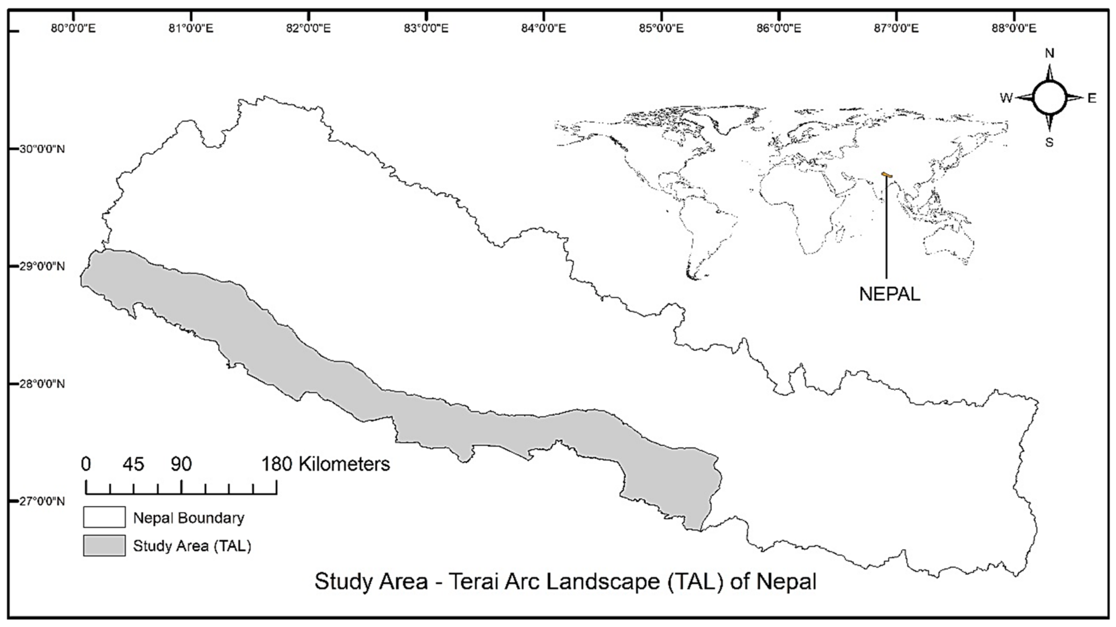
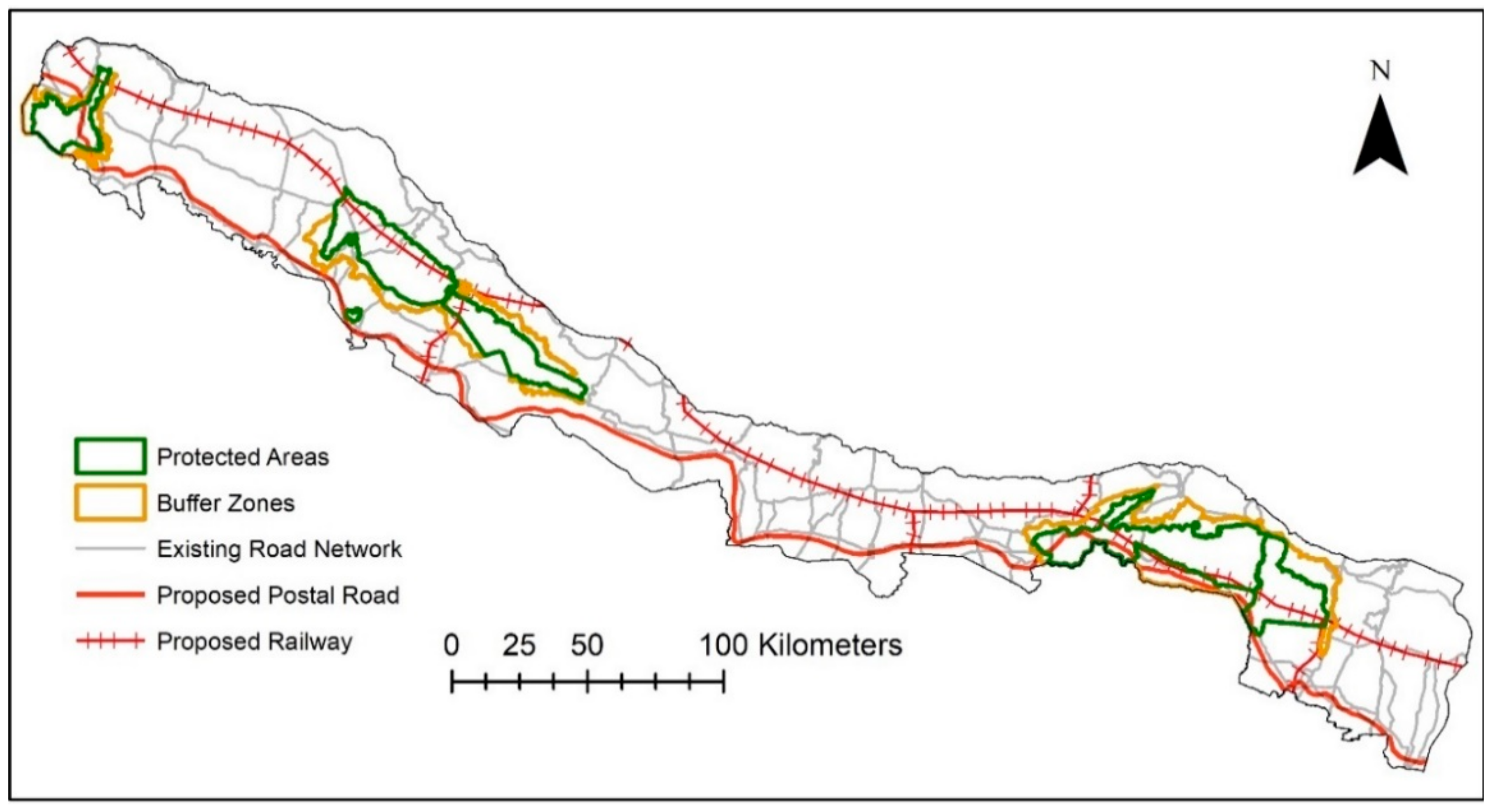
2.1. Study Area

Established in 2001, TAL is a transboundary landscape between Nepal and India and was based on the distribution of tigers along with other ecological characteristics. It extends along the Gangetic plain of India from Bagmati to Yamuna and includes 15 protected areas, 6 of which are located in Nepal. In Nepal, it stretches in the southern lowlands across 18 districts and occupies an area of 24,710 sq. km [22] (Figure 1). TAL harbours critical natural habitats supporting globally important biodiversity including some endangered wildlife. It holds meta-populations of important mega-fauna such as tiger, elephant, and rhinoceros. It also supports the highest human population densities and is among the most productive regions of Nepal. The six protected areas of TAL in Nepal are the following: five national parks (Chitwan National Park, Bardia National Park, Banke National Park, Suklaphanta National Park, and Parsa National Park) and a conservation area (Blackbuck Conservation Area). These protected areas are reinforced with adjacent buffer zones. The landscape is affected by many disturbances such as agriculture, settlements, and associated infrastructure.

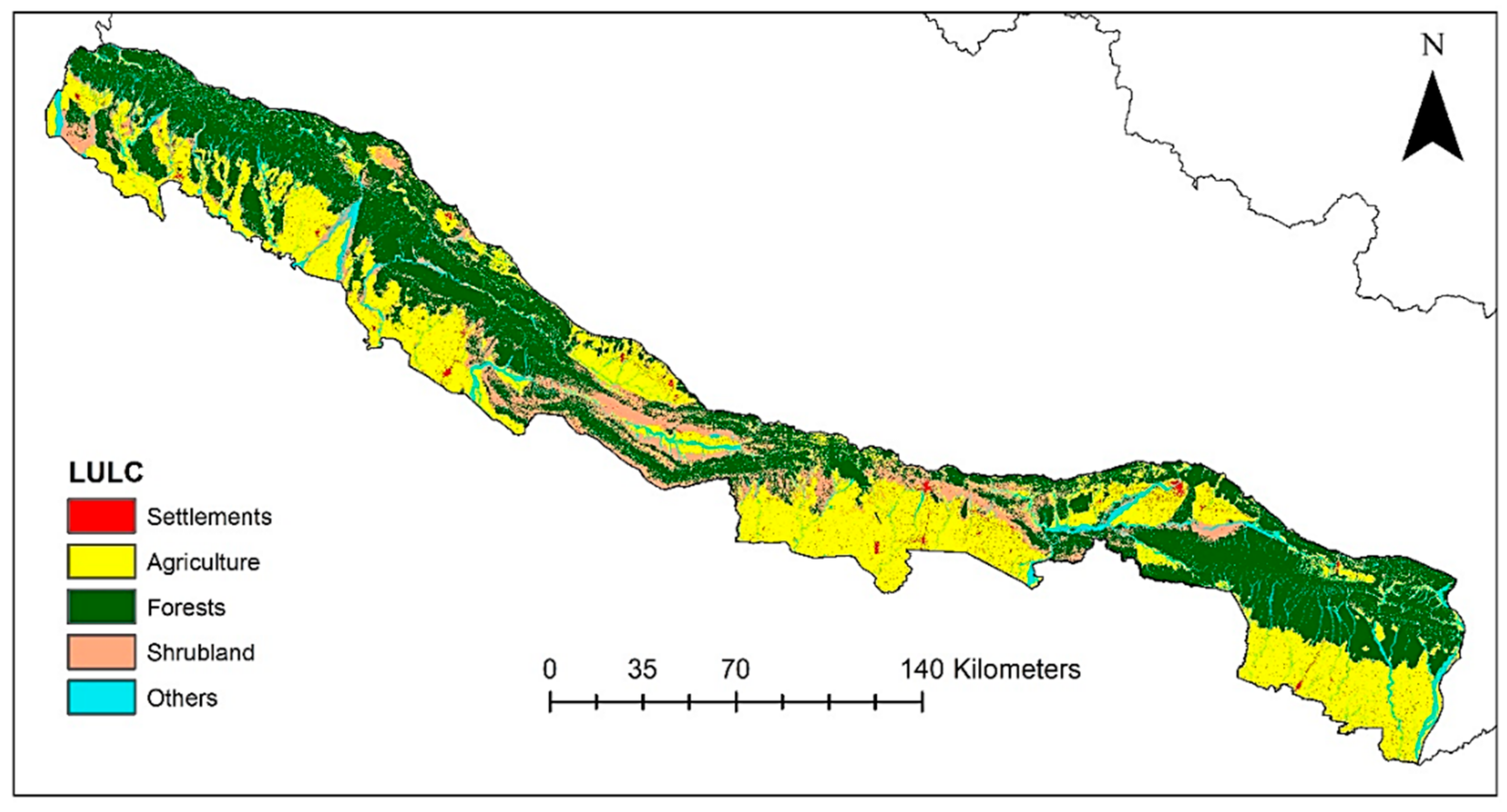
2.2. Data Collection and Processing

We used maximum cloud-free Landsat 8 Operational Land Imager images (OLI) from the year 2016 from the United State Geological Survey (USGS) (https://earthexplorer.usgs.gov). For land cover classification, four scenes (path/row: 141/41 dated 25 October, 142/41 dated 22 March, 143/ 41 dated 23 October, and 144/40 dated 1 and 17 February) were used. All images were verified for geometric accuracy and processed in environment for visualizing images (ENVI) [34]. During the analysis, scenes 144/40 were divided into two parts to remove the minor cloud cover area. After classification of LULC, all classified images were mosaiced and analyzed in ENVI environment. We developed five LULC classes; agriculture, forests, built-up, shrubland, and others (

Table 1. Land use and land cover classification scheme in the study area.

S.N.	Land Cover	Description
1.	Forests	Land dominated by trees (evergreen broad leaf forest and deciduous forest)
2.	Shrubland	Bush, grasslands, shrub cover, and degraded forests
3.	Agriculture	Land under cultivation of agricultural crops
4.	Built-up	Urban and rural settlements and commercial area
5.	Others	Water bodies, wetlands, barren lands/sand

). A supervised approach maximum likelihood algorithm was used for the classification of LULC [35]. The maximum likelihood approach is widely used in remote sensing [35]. Training samples for the classification were collected using high-resolution images from Google Earth (http://earth.google.com) and ground-truthed using global positioning system data during field visits and verification in 2016. The LULC accuracy assessment was verified using random sampling point and at least 50 sample points were sampled per LULC class per tile. The overall classification accuracy, user’s accuracy, and producer’s accuracy for the LULC maps are observed and a minimum of 84% to 88% of overall accuracy was identified.

Administrative boundary vector data were acquired from the Survey Department of Nepal [36]. Vector data for existing and proposed roads and railways were acquired from the Department of Roads and Department of Railways, respectively. Data for different InVEST parameters were extracted from studies that used the InVEST HQ model to map terrestrial biodiversity and adjusted using the data elicited from expert knowledge (Appendix A). We consulted experts with a background in biodiversity conservation and ecological modelling from government agencies and conservation organizations in Nepal. Details of the sources and parameter values are provided as supplementary materials (Appendix A).

2.3. GIS Based Modelling Using InVEST

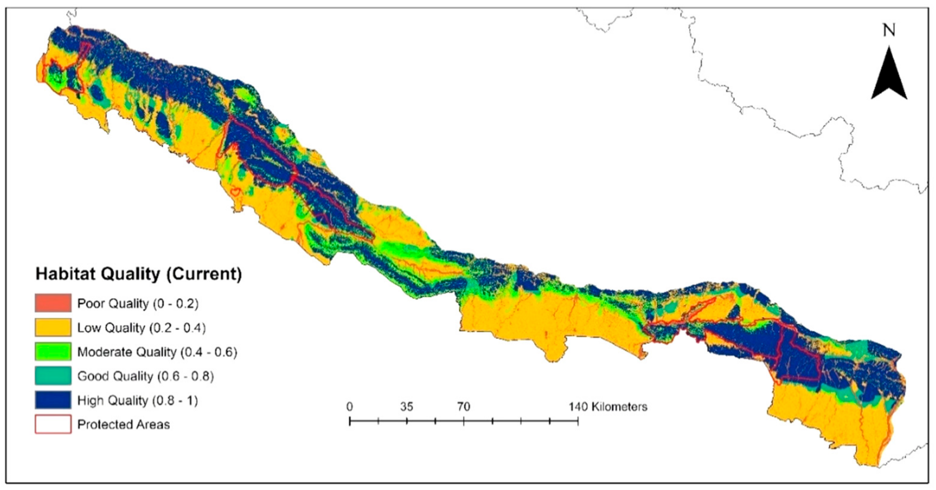
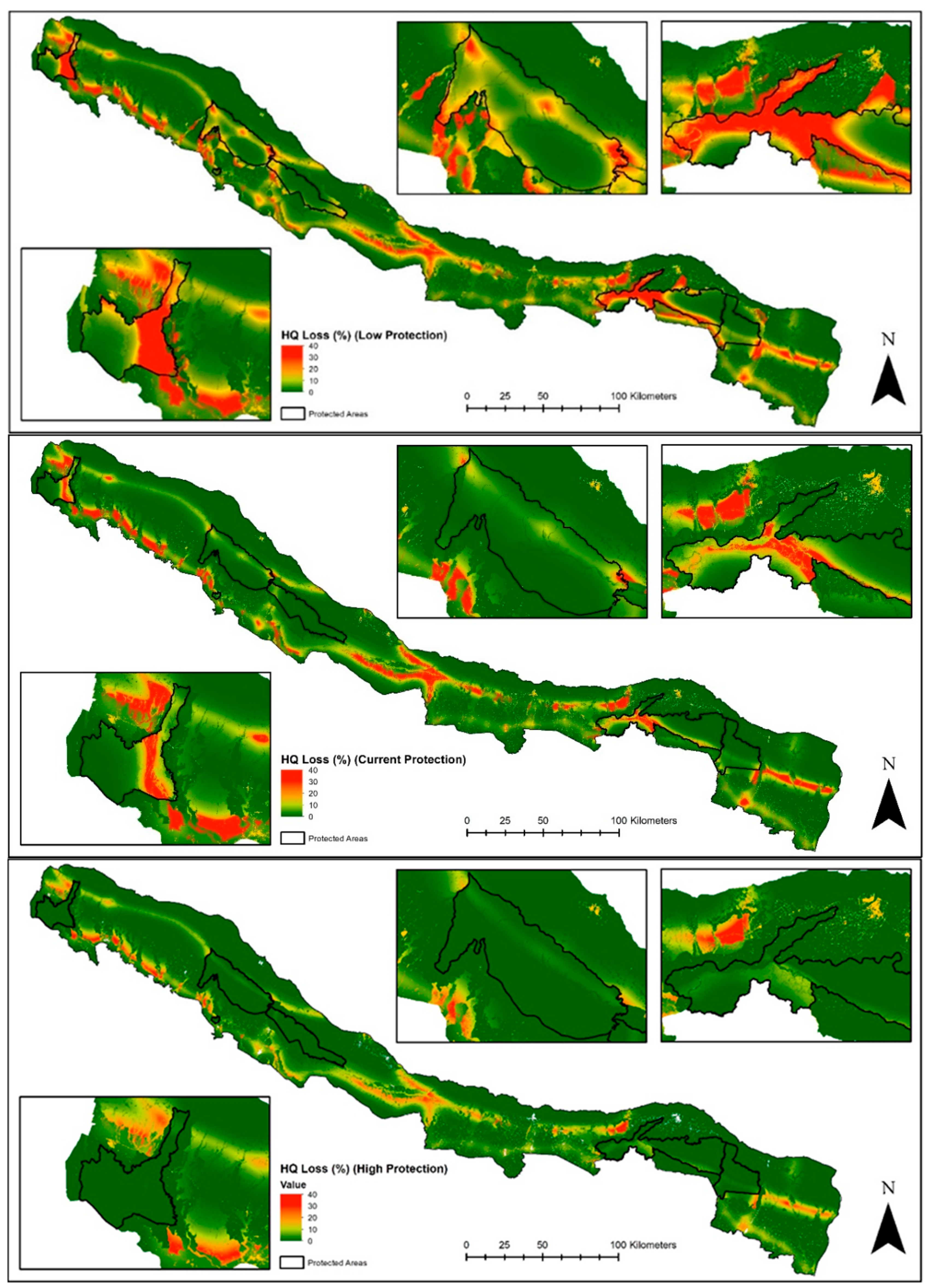
We used the spatially explicit habitat quality module of InVEST version 3.4.4 to model the change in distribution of habitat quality levels in three different protection level scenarios [37]. The model is based on the hypothesis that LULC types with higher habitat quality have higher richness of species and a lower or decline in habitat quality have a low persistence of species. The model considers habitat quality as a function of habitat suitability and four threat parameters; (i) the relative impact of each threat, (ii) the relative sensitivity of each habitat type to each threat, (iii) the distance between the habitats and sources of threats, and (iv) the degree to which the land is legally protected.

We considered general terrestrial biodiversity to determine whether the particular LULC type is considered a suitable habitat or not [38]. We assigned different habitat suitability scores (Hj) in the range of 0–1 for the five LULC classes (j) (Appendix A). The values for each class are relative to each other. Forest was assigned the terrestrial habitat type with the highest habitat suitability for native species as it is considered the least modified of the habitats, followed by shrublands and agriculture. Because we considered only general terrestrial biodiversity, the habitat suitability score for the LULC class ‘others’, which includes water bodies, wetlands, and barren lands, was assigned low values. Based on the literature and available data sources for the area, we selected four threats to biodiversity (i) agriculture, (ii) settlements, (iii) roads, and (iv) railways [39]. The source of each threat was mapped on a raster in which the value of the grid cell indicated the presence (1) or absence (0) of each threat. Four factors were used to determine the impact of each of these threats on the different habitat types.

First, the relative impact of each threat was determined to capture the different damage potentials of each threat on the habitat. The threat’s weight (w_r) is the relative impact score to all threats (i.e., if agriculture has a weight of 1 and settlement has a weight of 0.5, then agriculture causes degradation twice as much as the settlements). Second, the maximum effective distance of each threat was determined, that is, the maximum distance over which the threat affects habitat quality. If the habitat is within the impact distance of the threats, then it is within the threat’s degradation zone. The impact of each threat on habitat in general decreases as the distance from the threat source decreases. We used the exponential distance-decay rate, an indicative pattern seen in ecology [40], to explain how the spatial impact of the threat diminishes. For instance, if the maximum distance of the threat is set to 1 km, then its impact will decrease by about 50 percent on the habitat pixel that is at 200 m from the threat.

The impact of threat r that lies in the grid cell y, r_y, on habitat in grid cell x is given by i_rxy and is represented by the following equation:

$$i_{rxy}=\exp \left(-\left(\frac{2.99}{d_{r \max }}\right)d_{xy}\right)$$

(1)

where d_xy is the linear distance between grid cells x and y, and d_{r max} is the maximum effective distance of threat r.

Third, the level of accessibility to threats was determined. The model assumes that the greater physical, social, or legal protection the habitat pixel has, the less it will be affected by the nearby threats. β_x ∈ [0,1] indicates the level of accessibility in the grid cell x; where 1 indicates complete accessibility and 0 indicates no accessibility. The impact of the threat decreases with the decrease in the accessibility of the threat. We used the boundary of protected areas (PA^access) and buffer zones (BZ^access) as accessibility to threat layers. Buffer zones are human-dominated landscapes adjacent to protected areas that provide additional protection, but are subject to pressure from anthropogenic threats. Poaching, illegal logging, and invasive species continue to challenge protected areas in Nepal, so we estimate the existing level of accessibility to threats to be as follows: PA^access = 0.4 and BZ^access = 0.8. In addition, taking the reference of the existing protection levels, we assume lower protection scenario values to be PA^access = 0.8 and BZ^access = 1, and higher protection scenario values to be PA^access = 0.2 and BZ^access = 0.6.

Fourth, the relative sensitivity of the habitat to all of the threats was determined. The InVEST model assumes that the more sensitive a habitat is to a threat, the more degradation will occur in that habitat from the degradation source. For example, a forest habitat may suffer more degradation from adjacent agriculture (higher sensitivity) than disturbances from settlements (lower sensitivity).

$S_{jr}=\begin{array}{cc}\in & \left[0,1\right]\end{array}$ indicates the sensitivity of habitat type j to the threat r, where the values closer to 1 indicate greater sensitivity to the threat.

Further, the total threat level in the grid cell x with the habitat type j is calculated as D_{x j}.

$$\begin{gathered} D_{xj}={\displaystyle \sum }_{r=1}^R {\displaystyle \sum }_{y=1}^{Y_r}{w}_r{r}_{y }{i}_{rxy} {\beta }_x S_{jr} \\ {D}_{xj}={\displaystyle \sum }_{r=1}^R {\displaystyle \sum }_{y=1}^{Y_r}\left(\frac{w_{r }}{{{\displaystyle \sum }}_{r=1}^R{w}_r}\right)r_{y }{i}_{rxy} {\beta }_x S_{jr} \end{gathered}$$

(2)

where y indexes all grid cells on r’s raster map and Y_r indicates the set of grid cells on r’s raster map.

The quality of habitat in the parcel x of LULC j is Q_xy, where

$$Q_{xj}=H_j\left(1-\left(\frac{D_{xj}^z}{D_{xj}^z+k^z}\right)\right)$$

(3)

z and k are scaling parameters (or constants) used by the model.

Therefore, when Q_xj = 1, the quality of the habitat in the grid cell x is at its maximum. The model parameters and steps are detailed in the model guidebook [37].

Finally, we categorized the habitat quality scores for the landscape into five classes: poor (0–0.2), low (0.2–0.4), moderate (0.4–0.6), good (0.6–0.8), and high (0.8–1), and examined the resulting changes.

3. Results

The current and proposed infrastructure cross several ecosystems including those in protected areas (Figure 2). There is a considerable spatial variability in habitat quality across the landscape due to differences in land use and land cover (Figure 3), and the predicted effects of different threats in the landscape (Figure 4). As a result, the landscape is mainly dominated by both high and low habitat quality classes. At a landscape level, the proposed infrastructure will cause habitat quality losses primarily of the high-quality classes in all protection level scenarios; existing protection (770 km² or 8%), lower protection (1138 km² or 12%), and higher protection (584 km² or 6%) (

Table 2. Losses in habitat quality (HQ) scores in the landscape (“-” = No Loss).

HQ Classes	Existing Protection (S1)		Lower Protection (S2)		Higher Protection (S3)
	Area (km2)	% Loss	Area (km2)	% Loss	Area (km2)	% Loss
Poor (0–0.2)	-	-	-	-	-	-
Low (0.2–0.4)	-	-	-	-	-	-
Moderate (0.4–0.6)	−42	−1	-	-	−52	−2
Good (0.6–0.8)	-	-	-	-	-	-
High (0.8–1)	−770	−8	−1138	−12	−584	−6

). Habitat quality losses at pixel levels are more pronounced and reach up to 40% in several areas in each of the scenarios (Figure 5). The results suggest that the proposed infrastructure will cross and disproportionately degrade high quality habitat areas regardless of protection levels.

Our analysis of changes in habitat quality inside the protected areas and their adjacent buffer zones within TAL shows that habitat quality remains relatively intact in the high protection scenario when compared with other scenarios (

Table 3. Mean percent habitat quality loss in the protected areas and buffer zones.

Sn.	Protected Area and Buffer Zones	Existing Protection	Lower Protection	Higher Protection
		Mean (%) HQ Loss
1	Banke Buffer Zone	0.42	5.48	0.02
2	Banke National Park	0.79	3.49	0.12
3	Bardia Buffer Zone	0.23	8.23	0.04
4	Bardia National Park	1.99	5.78	0.54
5	Blackbuck Conservation Area	2.36	5.54	0.57
6	Chitwan Buffer Zone	0.98	8.81	0.06
7	Chitwan National Park	4.43	10.59	1.03
8	Parsa Buffer Zone	0.37	7.36	0.03
9	Parsa National Park	1.69	3.47	0.54
10	Suklaphanta Buffer Zone	0.70	5.90	0.09
11	Suklaphanta National park	5.41	13.33	0.13

). In the existing protection scenario, the loss in mean habitat quality is notable in the protected areas and is relatively higher than the buffer zones: for example, losses in Suklaphanta NP, Chitwan NP, and Blackbuck Conservation Area. However, in the low protection scenario, large losses are experienced in both the protected areas and their buffer zones. This finding suggests that different levels of protection have a varied impact of infrastructure on the protected areas and their buffer zones. While increasing the current levels of protection within the protected areas and buffer zones will contribute to preventing some levels of habitat quality loss, further decreases in protection levels will cause significant loss.

4. Discussion and Conclusion

We show that although there is a large proportion of the TAL that provides a suitable habitat for biodiversity conservation, the area is under pressure from different anthropogenic threats, resulting in a large spatial heterogeneity in habitat quality across the landscapes. In particular, the proposed new road and rail infrastructure are predicted to reduce habitat quality in pixel levels by up to 40% in three main areas within and close to current National Parks, as shown in Figure 5. As many large mammals, such as tiger and rhino, require large areas for conservation, the long-term viability of their populations may be threatened as a result of habitat loss and fragmentation, particularly in these three focal areas. Although increasing the level of protection in the protected areas may mitigate degradation within the protected areas at some levels, other biologically important areas such as the high-quality habitat areas shown in our study will still be vulnerable to degradation. In addition, the identification of hotspots for habitat quality loss could be used to best orient conservation efforts to the most vulnerable sites in the landscape. This information is critical to align the current conservation efforts of the Government of Nepal such as in maintaining corridor connectivity, bottlenecks, protection forests, and community forests.

There is growing evidence showing the negative impact of infrastructure such as roads and railways on habitat quality [11,41]. Our findings are consistent with several other similar spatial modelling studies. Sallustio, et al. [42] found that habitat quality depends on the location of anthropogenic threats such as urban areas and roads, and decreases when areas are more accessible or less restrictive. They confirm that high levels of protection ensure improved conservation outcomes. Others have similarly recorded the spatial distribution of habitat quality losses in biologically rich areas due to anthropogenic threats such as in Central Kalimantan of Indonesia [32].

We recognize that our study has several limitations. Although there are a number of threats that may affect the landscape [22], we only considered a limited number of threats such as agriculture, settlements, and infrastructure because we lacked data for other threats. Further, the model assumes that each threat will have similar degradation impacts. However, in reality, each threat will have different levels of impact and will most likely act synergistically [43]. As well as the immediate loss of habitat, new infrastructure can have a long-term impact on the biodiversity by increasing economic activities and the spread of settlements [44]. The TAL continues to face pressure due to unprecedented growth in human population and urban expansion [35] and further infrastructure development will escalate this process. Our study did not capture these factors. We acknowledge these as major limitations of this study. Thus, our findings could be further enhanced by utilizing other threat data and modeling population growth and economic activities. This would provide a more refined evaluation of the impact of new infrastructure on biodiversity.

Further, although we considered habitat suitability for biodiversity, we did not examine how individual species will be affected. In the future, modelling could be improved by using species-specific data to develop habitat suitability models for key species. This could give data of a finer resolution on how each species and their habitats will be affected by the proposed infrastructure. However, at this stage, there are limited data and resources to conduct such detailed analysis. As infrastructure development in Nepal is on-going, our primary goal was to reveal a first rapid assessment of impact of such infrastructure on general terrestrial biodiversity. Although there are several limitations, our study added to the dimension of using readily available GIS based data to quantify the impact of infrastructure development. This methodology will help other researchers to conduct studies in other countries, particularly developing countries, where there is scarcity of data and resources to conduct a detailed analysis.

Poorly planned infrastructure development will not only have immediate consequences for biodiversity, but also increase the risk of permanently locking continuous threats to biodiversity for the future. Traditional environmental impact assessments (EIAs), generally fast and based on inadequate data, are sometimes seen as short-sighted in showing the full extent of negative consequences of infrastructure development [18]. An integration of best practice in environmental planning such as strategic environmental assessments (SEAs), which have broader spatial and temporal focus than EIAs [45], and other proactive land use and infrastructure planning, are more desirable [18]. We suggest our assessment of habitat quality can be used as a basis for developing a more detailed SEA. We recommend that policymakers, development planners, and conservation agencies consider habitat quality during the spatial planning process and work together to ensure that proper environmental planning is followed. In fact, given the importance of biodiversity in the landscape and to honor current conservation commitments, we strongly recommend integrating biodiversity conservation in planning and implementing infrastructure development in the region.

References

1. MEA. Ecosystems and Human Well-Being: A Framework for Assessment; Island Press: Washington, DC, USA, 2005; ISBN 1-55963-403-0. [Google Scholar]
2. Pimm, S.L.; Russell, G.J.; Gittleman, J.L.; Brooks, T.M. The future of biodiversity. Science 1995, 269, 347–350. [Google Scholar] [CrossRef] [PubMed]
3. Sala, O.E.; Chapin, F.S., 3rd; Armesto, J.J.; Berlow, E.; Bloomfield, J.; Dirzo, R.; Huber-Sanwald, E.; Huenneke, L.F.; Jackson, R.B.; Kinzig, A.; et al. Global biodiversity scenarios for the year 2100. Science 2000, 287, 1770–1774. [Google Scholar] [CrossRef] [PubMed]
4. UNEP. Global Environment Outlook (Geo-5): Environment for the Future We Want; Progress Press: Valletta, Malta, 2012; ISBN 978-92-807-3177-4. [Google Scholar]
5. Thomas, C.D.; Cameron, A.; Green, R.E.; Bakkenes, M.; Beaumont, L.J.; Collingham, Y.C.; Erasmus, B.F.N.; de Siqueira, M.F.; Grainger, A.; Hannah, L.; et al. Extinction risk from climate change. Nature 2004, 427, 145–148. [Google Scholar] [CrossRef] [PubMed] [Green Version]
6. Butchart, S.H.; Walpole, M.; Collen, B.; van Strien, A.; Scharlemann, J.P.; Almond, R.E.; Baillie, J.E.; Bomhard, B.; Brown, C.; Bruno, J.; et al. Global biodiversity: Indicators of recent declines. Science 2010, 328, 1164–1168. [Google Scholar] [CrossRef] [PubMed]
7. Alkemade, R.; van Oorschot, M.; Miles, L.; Nellemann, C.; Bakkenes, M.; Ten Brink, B. Globio3: A framework to investigate options for reducing global terrestrial biodiversity loss. Ecosystems 2009, 12, 374–390. [Google Scholar] [CrossRef]
8. Richardson, M.L.; Wilson, B.A.; Aiuto, D.A.S.; Crosby, J.E.; Alonso, A.; Dallmeier, F.; Golinski, G.K. A review of the impact of pipelines and power lines on biodiversity and strategies for mitigation. Biodivers. Conserv. 2017, 26, 1801–1815. [Google Scholar] [CrossRef]
9. Laurance, W.F.; Clements, G.R.; Sloan, S.; O’Connell, C.S.; Mueller, N.D.; Goosem, M.; Venter, O.; Edwards, D.P.; Phalan, B.; Balmford, A.; et al. A global strategy for road building. Nature 2014, 513, 229–232. [Google Scholar] [CrossRef] [PubMed]
10. Ibisch, P.L.; Hoffmann, M.T.; Kreft, S.; Pe’er, G.; Kati, V.; Biber-Freudenberger, L.; DellaSala, D.A.; Vale, M.M.; Hobson, P.R.; Selva, N. A global map of roadless areas and their conservation status. Science 2016, 354, 1423–1427. [Google Scholar] [CrossRef] [PubMed]
11. Trombulak, S.C.; Frissell, C.A. Review of ecological effects of roads on terrestrial and aquatic communities. Conservat. Biol. 2000, 14, 18–30. [Google Scholar] [CrossRef]
12. Moran, M.D.; Cox, A.B.; Wells, R.L.; Benichou, C.C.; McClung, M.R. Habitat loss and modification due to gas development in the Fayetteville shale. Environ. Manag. 2015, 55, 1276–1284. [Google Scholar] [CrossRef] [PubMed]
13. Jaeger, J.A.; Bowman, J.; Brennan, J.; Fahrig, L.; Bert, D.; Bouchard, J.; Charbonneau, N.; Frank, K.; Gruber, B.; von Toschanowitz, K.T. Predicting when animal populations are at risk from roads: An interactive model of road avoidance behavior. Ecol. Model 2005, 185, 329–348. [Google Scholar] [CrossRef]
14. Geneletti, D. Biodiversity impact assessment of roads: An approach based on ecosystem rarity. EIA Rev. 2003, 23, 343–365. [Google Scholar] [CrossRef]
15. González, A.; Keneghan, D.; Fry, J.; Hochstrasser, T. Current practice in biodiversity impact assessment and prospects for developing an integrated process. Impact Assess Proj. Apprais. 2014, 32, 31–42. [Google Scholar] [CrossRef]
16. Forman, R.T.T.; Sperling, D.; Bissonette, J.A.; Clevenger, A.P.; Cutshall, C.D.; Dale, V.H.; Fahrig, L.; France, R.L.; Heanue, K.; Goldman, C.R.; et al. Road Ecology: Science and Solutions; Island Press: Washington, DC, USA, 2003; ISBN 1559639334. [Google Scholar]
17. Laurance, W.F.; Goosem, M.; Laurance, S.G. Impacts of roads and linear clearings on tropical forests. Trends Ecol. Evol. 2009, 24, 659–669. [Google Scholar] [CrossRef] [PubMed] [Green Version]
18. Laurance, W.F.; Arrea, I.B. Roads to riches or ruin? Science 2017, 358, 442–444. [Google Scholar] [CrossRef] [PubMed]
19. Lechner, A.M.; Chan, F.K.S.; Campos-Arceiz, A. Biodiversity conservation should be a core value of China’s belt and road initiative. Nat. Ecol. Evol. 2018, 2, 408–409. [Google Scholar] [CrossRef] [PubMed]
20. Dhakal, M.; Baral, H. Tiger conservation in South Asia: Lessons from terai arc landscapes, nepal. In Proceedings of the 2nd International Conference on Tropical Biology Ecological Restoration in Southeast Asia: Challenges, Gains, and Future Directions, SEAMEO BIOTROP, Bogor, Indonesia, 12–13 October 2016. [Google Scholar]
21. Thapa, K.; Wikramanayake, E.; Malla, S.; Acharya, K.P.; Lamichhane, B.R.; Subedi, N.; Pokharel, C.P.; Thapa, G.J.; Dhakal, M.; Bista, A.; et al. Tigers in the terai: Strong evidence for meta-population dynamics contributing to tiger recovery and conservation in the Terai Arc Landscape. PLoS ONE 2017, 12, e0177548. [Google Scholar] [CrossRef] [PubMed]
22. Ministry of Forests and Soil Conservation. Strategy and Action Plan 2015–2025, Terai Arc Landscape, Nepal; Ministry of Forests and Soil Conservation: Kathmandu, Nepal, 2015.
23. Atkinson, G.; Bateman, I.; Mourato, S. Recent advances in the valuation of ecosystem services and biodiversity. Oxf. Rev. Econ. Policy 2012, 28, 22–47. [Google Scholar] [CrossRef]
24. Baral, H.; Keenan, R.J.; Sharma, S.K.; Stork, N.E.; Kasel, S. Economic evaluation of ecosystem goods and services under different landscape management scenarios. Land Use Policy 2014, 39, 54–64. [Google Scholar] [CrossRef]
25. Zlinszky, A.; Heilmeier, H.; Balzter, H.; Czúcz, B.; Pfeifer, N. Remote sensing and GIS for habitat quality monitoring: New approaches and future research. Remote Sens. 2015, 7, 7987–7994. [Google Scholar] [CrossRef] [Green Version]
26. Corbane, C.; Lang, S.; Pipkins, K.; Alleaume, S.; Deshayes, M.; Millán, V.E.G.; Strasser, T.; Borre, J.V.; Toon, S.; Michael, F. Remote sensing for mapping natural habitats and their conservation status—New opportunities and challenges. Int. J. Appl. Earth Obs. Geoinf. 2015, 37, 7–16. [Google Scholar] [CrossRef]
27. Turner, W.; Spector, S.; Gardiner, N.; Fladeland, M.; Sterling, E.; Steininger, M. Remote sensing for biodiversity science and conservation. Trends Ecol. Evol. 2003, 18, 306–314. [Google Scholar] [CrossRef]
28. Johnson, M.D. Measuring habitat quality: A review. Condor 2007, 109, 489–504. [Google Scholar] [CrossRef]
29. Lengyel, S.; Déri, E.; Varga, Z.; Horváth, R.; Tóthmérész, B.; Henry, P.; Kobler, A.; Kutnar, L.; Babij, V.; Seliškar, A.; et al. Habitat monitoring in Europe: A description of current practices. Biodivers. Conserv. 2008, 17, 3327–3339. [Google Scholar] [CrossRef]
30. Johnson, M.D.; Arcata, C. Habitat quality: A brief review for wildlife biologists. Trans. West. Sect. Wildl. Soc. 2005, 41, 31. [Google Scholar]
31. Corsi, F.; De Leeuw, J.; Skidmore, A. Modeling species distribution with GIS. In Research Techniques in Animal Ecology, 1st ed.; Boitani, L., Fuller, T., Eds.; Columbia University Press: New York, NY, USA, 2000; pp. 389–434. ISBN 0-231-11340-4. [Google Scholar]
32. Sharma, R.; Nehren, U.; Rahman, S.A.; Meyer, M.; Rimal, B.; Seta, G.A.; Baral, H. Modeling land use and land cover changes and their effects on biodiversity in Central Kalimantan, Indonesia. Land 2018, 7, 1–14. [Google Scholar] [CrossRef]
33. Baral, H.; Jaung, W.; Bhatta, L.D.; Phuntsho, S.; Sharma, S.; Paudyal, K.; Zarandian, A.; Sears, R.; Sharma, R.; Dorji, T.; et al. Approaches and Tools for Assessing Mountain Forest Ecosystem Services. Available online: http://www.cifor.org/publications/pdf_files/WPapers/WP235Baral.pdf (accessed on 20 July 2018).
34. Rimal, B.; Zhang, L.; Keshtkar, H.; Wang, N.; Lin, Y. Monitoring and modeling of spatiotemporal urban expansion and land-use/land-cover change using integrated markov chain cellular automata model. ISPRS 2017, 6, 288. [Google Scholar] [CrossRef]
35. Rimal, B.; Zhang, L.; Stork, N.; Sloan, S.; Rijal, S. Urban expansion occurred at the expense of agricultural lands in the tarai region of Nepal from 1989 to 2016. Sustainability 2018, 10, 1341. [Google Scholar] [CrossRef]
36. Ministry of Land Resource and Management. Topographical Map; Government of Nepal, Ministry of Land Resource and Management, Survey Department, Topographic Survey Branch: Kathmandu, Nepal, 1995.
37. Sharp, R.; Tallis, H.T.; Ricketts, T.; Guerry, A.D.; Wood, S.A.; Chaplin-Kramer, R.; Nelson, E.; Ennaanay, D.; Wolny, S.; Olwero, N.; et al. InVEST 3.4.4 User’s Guide. Available online: http://data.naturalcapitalproject.org/invest-releases/3.4.4.post136+h96058b17dddb/userguide/ (accessed on 20 July 2018).
38. Polasky, S.; Nelson, E.; Pennington, D.; Johnson, K.A. The impact of land-use change on ecosystem services, biodiversity and returns to landowners: A case study in the state of minnesota. Environ. Ecol. Econ. 2010, 48, 219–242. [Google Scholar] [CrossRef]
39. Ministry of Forests and Soil Conservation. Nepal Fifth National Report to Convention on Biological Diversity; Government of Nepal, Ministry of Forests and Soil Conservation, Environment Division: Kathmandu, Nepal, 2014.
40. Nekola, J.C.; White, P.S. The distance decay of similarity in biogeography and ecology. J. Biogeogr. 1999, 26, 867–878. [Google Scholar] [CrossRef]
41. Rytwinski, T.; Fahrig, L. The impacts of roads and traffic on terrestrial animal populations. In Handbook of Road Ecology, 1st ed.; van der Ree, R., Smith, D.J., Grilo, C., Eds.; John Wiley & Sons, Ltd.: Hoboken, NJ, USA, 2015; pp. 237–246. ISBN 9781118568170. [Google Scholar]
42. Sallustio, L.; De Toni, A.; Strollo, A.; Di Febbraro, M.; Gissi, E.; Casella, L.; Geneletti, D.; Munafò, M.; Vizzarri, M.; Marchetti, M. Assessing habitat quality in relation to the spatial distribution of protected areas in Italy. J. Environ. Manag. 2017, 201, 129–137. [Google Scholar] [CrossRef] [PubMed]
43. Brook, B.W.; Sodhi, N.S.; Bradshaw, C.J. Synergies among extinction drivers under global change. Trends Ecol. Evol. 2008, 23, 453–460. [Google Scholar] [CrossRef] [PubMed]
44. Kasraian, D.; Maat, K.; Stead, D.; van Wee, B. Long-term impacts of transport infrastructure networks on land-use change: An international review of empirical studies. Transp. Rev. 2016, 36, 772–792. [Google Scholar] [CrossRef]
45. Fischer, T.B. The Theory and Practice of Strategic Environmental Assessment: Towards a More Systematic Approach, 1st ed.; Routledge: London, UK, 2007; p. 208. ISBN 1844074528. [Google Scholar]
46. Baral, H.; Keenan, R.J.; Sharma, S.K.; Stork, N.E.; Kasel, S. Spatial assessment and mapping of biodiversity and conservation priorities in a heavily modified and fragmented production landscape in North-Central Victoria, Australia. Ecol. Indic. 2014, 36, 552–562. [Google Scholar] [CrossRef]
47. Liang, Y.; Liu, L. Simulating land-use change and its effect on biodiversity conservation in a watershed in Northwest China. EHS 2017, 3, 1335933. [Google Scholar] [CrossRef]
48. Kuhnert, P.M.; Martin, T.G.; Griffiths, S.P. A guide to eliciting and using expert knowledge in bayesian ecological models. Ecol. Lett. 2010, 13, 900–914. [Google Scholar] [CrossRef] [PubMed]
Figure 1. Map of Terai Arc Landscape.
Ijgi 07 00365 g001
Figure 2. Protected areas and current and proposed infrastructure network of the Terai Arc Landscape.
Ijgi 07 00365 g002
Figure 3. Land use and land cover (LULC) of the Terai Arc Landscape.
Ijgi 07 00365 g003
Figure 4. Spatial distribution of current habitat quality in Terai Arc Landscape.
Ijgi 07 00365 g004
Figure 5. Habitat quality (HQ) loss (in percent) for three protection level scenarios (low protection, current protection, and high protection) with insets for three areas that are precited to be most affected by new infrastructure development.
Ijgi 07 00365 g005