Article

Extraction of Terrain Feature Lines from Elevation Contours Using a Directed Adjacent Relation Tree

Chinese Academy of Surveying and Mapping, Beijing 100830, China
*
Author to whom correspondence should be addressed.
ISPRS Int. J. Geo-Inf. 2018, 7(5), 163; https://doi.org/10.3390/ijgi7050163
Submission received: 15 March 2018 / Revised: 19 April 2018 / Accepted: 20 April 2018 / Published: 24 April 2018

Abstract

:
The extraction of terrain feature lines is an important yet challenging problem in the processing and usage of contour lines. Most research has focused on identifying terrain feature points by using methods such as the Douglas–Peucker (D–P) algorithm and on determining contour adjacent relations for closed contour lines by using methods such as Delaunay triangulation and its dual Voronoi diagram, with few attempts made to address open contour lines and identify the direction of contour lines. Here, we propose a novel method for terrain feature line extraction based on adjacent relation trees. First, a contour adjacent relation tree is constructed. The tree is used to determine the directions of closed and open contour lines and thereby form a “directed adjacent relation tree” (DART). Terrain feature points are then extracted using the classic D–P algorithm, followed by the identification and connection of valley and ridge points via the aforementioned DART. Finally, integrity compensation for terrain feature lines is performed based on a slope extension algorithm. The effectiveness and accuracy of this method is verified by experimental results obtained from 1:10,000 topographic map data.

1. Introduction

Terrain feature lines describe the skeletal structure of a terrain and they are the basis for a variety of important applications, including terrain analysis [1], contour generalization [2,3,4], and hydrologic analysis [5]. Thus, the automatic extraction of terrain feature lines has become a hot topic in topographic research [6,7,8], with researchers all over the world conducting many related studies in recent years. One of the most common approaches in these studies is to begin by detecting feature points according to terrain geometry and then to construct terrain feature lines by connecting strongly hierarchical and symmetrical feature points that lie on adjacent contour lines (contours) [5,9]. Methods of terrain feature line extraction may be divided into two types based on the data source used for the detection and connection of feature points, namely, DEM-based [1,10] and contour-based methods [11,12]. This study falls in the latter category. There are two forms of contour lines in the database of topographic maps: open contours and closed contours. The surface of closed contours is unambiguous. In contrast, the surface of open contours is ambiguous. Methods of contour-based terrain feature line extraction depend on two fundamental processes: the detection of contour adjacent relations and the determination of contour directions for closed and open contours within a map. The former ensures that we can reduce the search range when connecting feature points, whereas the latter ensures that ridge and valley points can be accurately distinguished.
Currently, the methods for determining contour adjacent relations are derived from the following four approaches: the geometric calculation method, the Voronoi diagrams method, the Delaunay triangulation method, and the region expansion method.
  • Geometric calculation method [13,14,15]: The inclusion relationships between the areas contained by contour lines are calculated to determine the “parent–child” hierarchies of the contours, which are subsequently used to identify contour adjacencies. Methods of this type are intuitive and easy to understand; however, they are unsuitable for maps that contain open contour lines.
  • Voronoi diagrams method [16]: Contour adjacent relations are identified through the first-order adjacencies of the contour line Voronoi diagram.
  • Delaunay triangulation method [17,18]: The edges of the triangles generated in Delaunay triangulation can also be used to identify adjacencies between contour lines. However, owing to the nested nature of the contours, the triangles generated from individual contour lines will cross the adjacent contours, which can lead to erroneous adjacent relation judgments. Poorten and Jones [17] proposed recognizing contour adjacencies based on constrained Delaunay triangulation, which effectively prevents the triangles from crossing polygons, thus ensuring the accuracy of contour adjacent relation judgments.
  • As Voronoi diagrams and constrained Delaunay triangulation are not affected by open contour lines, these methods are widely applicable for the judgment of contour adjacencies. However, both methods are inefficient when processing contours over a large area because they consume large amounts of time during spatial meshing computations and searches for associated contour pairs.
  • Region expansion method [19]: The region expansion method operates under the following premise. As contour lines expand, the intersection of the expanded boundaries with other contour lines indicates that the intersecting contour lines are adjacent to each other. This method does not rely on the elevation of a contour, but if an area contains open contour lines, the judgment of adjacent relations using this method is susceptible to errors.
The Douglas–Peucker (D–P) algorithm [20] is a classic line simplification algorithm. The algorithm effectively identifies curved feature points by setting a suitable distance threshold. Many researchers use the D–P algorithm as a topographic feature point extraction method [21]. After recognizing terrain feature points, contour directions are important references for differentiating between concave and convex feature points on a contour line [22]. Contour line direction reflects the direction of elevation change between contours. When the elevation of the contours increases, progressing forward, the contour directions point left, while decreasing elevation is indicated by contour directions pointing to the right [23,24,25]. Most studies assume that the directions of all contours are correct when used as input for the extraction of terrain feature lines. However, in actual topographic map databases, most contour directions are not ordered. The directions of closed contour lines are easy to adjust, but the direction of open contour lines can be ambiguous. This ambiguity has been a persistent challenge for this field of cartography. In studies on open contours, researchers have proposed the use of map boundary distances to group open contour lines as closed contour lines, thus determining their directions of closure. The adjacent relation and elevational relationships between contours have also been used to unite open contours as closed contours [26]. In the methods just described, open contours are generally converted to closed contours for further consideration. However, these methods tend to be inaccurate in complex scenarios that involve a large number of open contour lines in a map.
In summary, current methods for the identification of terrain feature points from contours and contour adjacencies are generally based on Delaunay triangulation and its dual, the Voronoi diagram, or on the D–P algorithm. However, the extraction of terrain feature lines using Delaunay triangulation and Voronoi diagrams is inefficient and often leads to the extraction of redundant feature points. Furthermore, the D–P algorithm is limited to the extraction of terrain feature points and requires contour directions for the differentiation of ridge and valley points. Moreover, as the D–P algorithm cannot be used to recognize adjacent relations, the algorithm is incapable of constructing terrain feature lines by connecting terrain feature points. Considering that the detection of contour adjacent relations and the determination of contour directions are important elements in the automatic extraction of terrain feature lines, this paper introduces a new method of terrain feature line extraction based on adjacent relation trees. The aim of this paper is to contribute to the area of contour application research by developing an efficient and accurate method for automatic terrain feature line extraction that processes both closed and open contour lines.
The remainder of this paper is organized as follows. Section 2 presents the overall framework of our proposed method. Section 3 outlines the algorithm of construction of directed adjacent relation trees. Section 4 details the proposed terrain feature line extraction method using the directed adjacent relation trees. Section 5 discusses the experiments and analyses. Section 6 presents concluding remarks.

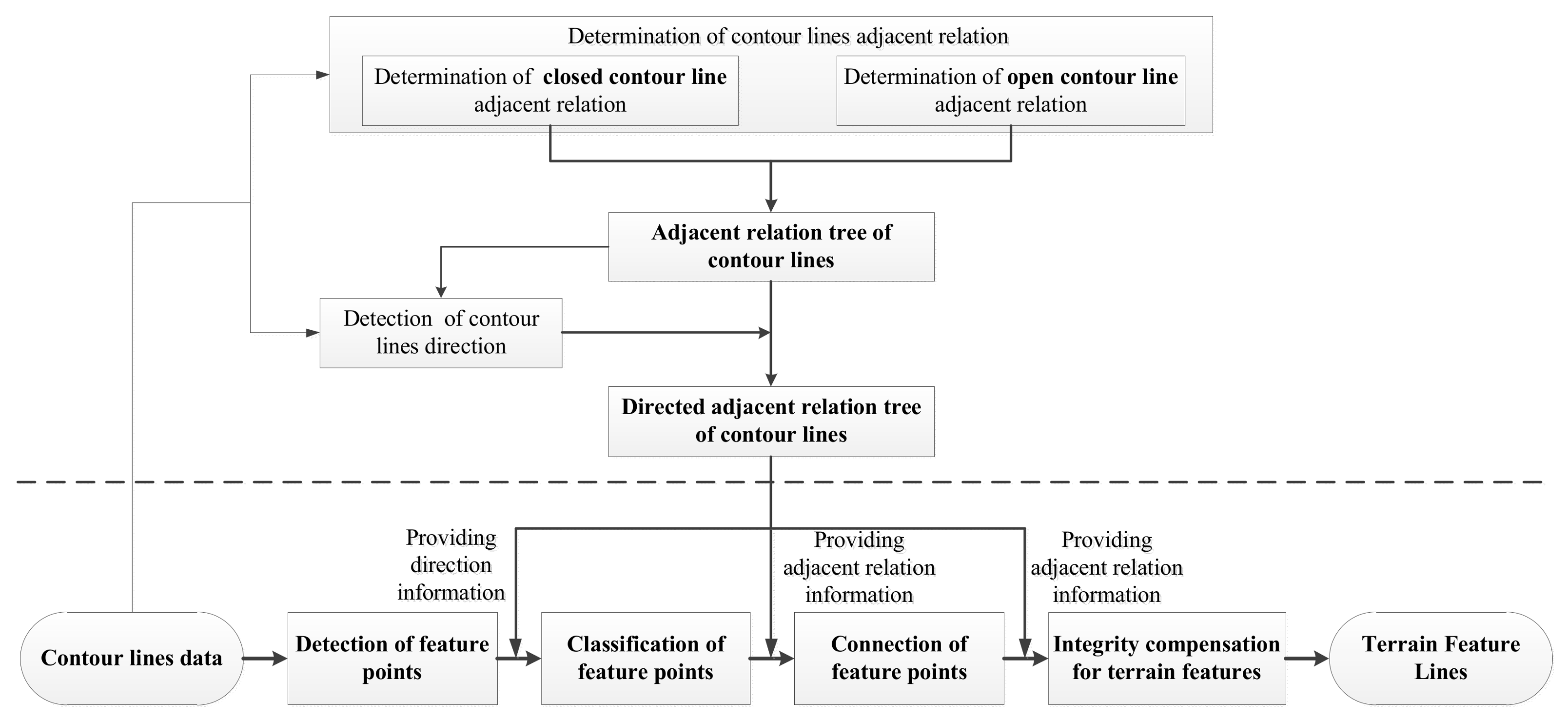
2. Framework for Terrain Feature Line Extraction Method

As depicted in the four boxes beneath the dotted line in Figure 1, our proposed method for terrain feature line extraction is composed of four steps:
(1)
Detect feature points using the D–P algorithm.
(2)
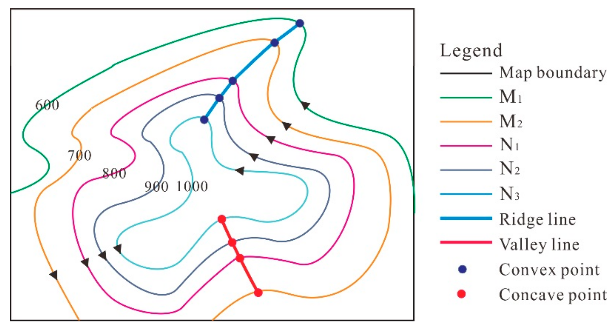
Classify each feature point as one of two types, concave or convex, which correspond to valley and ridge points in positive landforms.
(3)
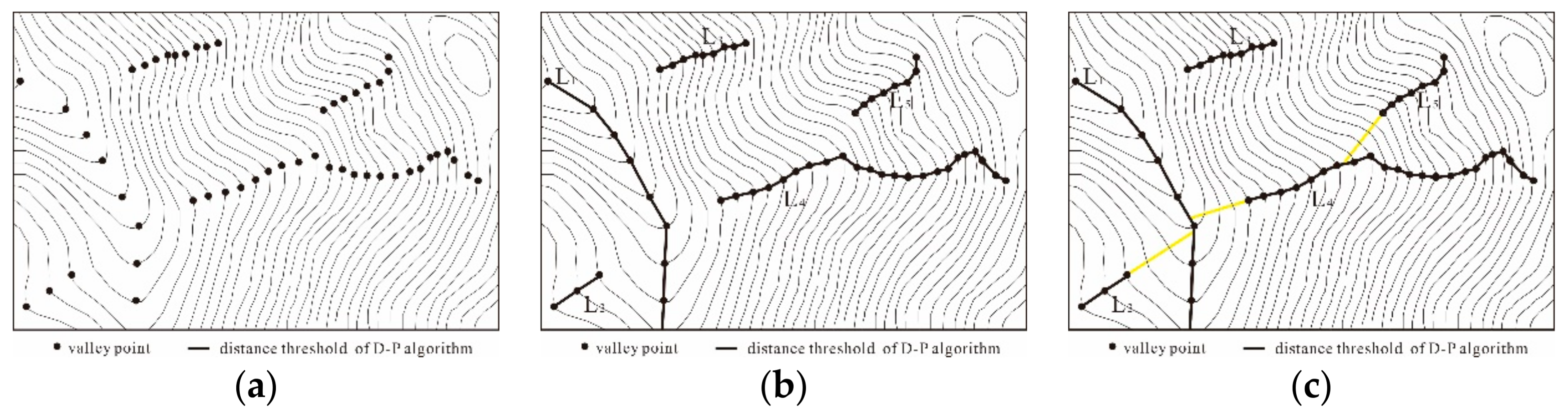
Connect feature points based on connection principles to form initial terrain feature lines.
(4)
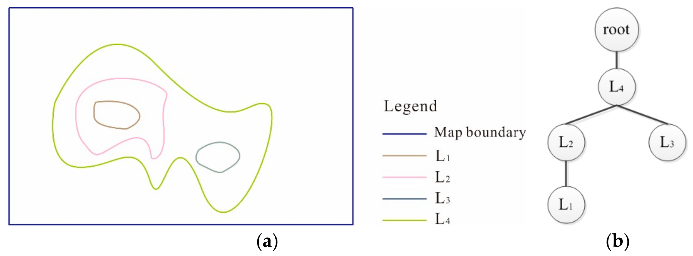
Perform integrity compensation for terrain features to form the final complete terrain feature lines, which possess tree structures.
Our proposed method for terrain feature line extraction is based on the “directed adjacent relation tree” (DART), depicted above the dotted line in Figure 1. The directed adjacent relation tree consists of two processes: the determination of adjacent relation and the detection of direction for contour lines. The algorithms used in the former process vary depending on whether the contour line is closed or open. Once constructed, the directed adjacent relation tree provides the information necessary to execute our method, furnishing direction information when feature points are classified, adjacent relation information when the feature points are connected, and integrity compensation for terrain features.

3. Construction of Directed Adjacent Relation Tree (DART)

A contour line may be treated as the combination of a curve, Li, and the area it contains, Pi [27]. In this context, the contour adjacent relation simply refers to the topological adjacent relation. As closed and open contours differ significantly in geometric structure, different adjacent relation judgment algorithms are applied to each contour type. We identify open contours by determining whether a contour intersects the boundaries of the map. Adjacent relation trees have been used to record the adjacencies between contours in their respective categories [28,29]. The nodes and edges of an adjacent relation tree represent the contours and adjacencies between the contours, respectively, whereas the singular root node of the tree represents the whole map.

3.1. Closed Contours

3.1.1. Determination of Adjacent Relation

The structures of closed contours are usually more regular and intact than those of open contours, and inter-contour relationships can be converted to surface-to-surface relationships. Hence, the judgment of adjacencies between contours can be treated as the judgment of inclusion relationships between surface elements. The judgment of an adjacent relation may therefore be described as follows:
If A P i < A P j and P i P j , where Li and Lj represent any two contours, Pi and Pj represent the physical areas contained by Li and Lj, and A P j represents the area calculation of Pj, with i ≠ j, then place Lj in the set of contours containing Li.
If Ln is the contour that has the smallest surface area in the set, then Li and Ln are adjacent contours, with Li being internally adjacent to Ln and Ln being externally adjacent to Li. If Li and Lm, the other contours, are both internally adjacent to Ln, then Li and Lm are parallel-adjacent.

3.1.2. Branched Tree of Closed Contours

The closed contours are organized according to the size of the area that each contains, in ascending order, to form a candidate set R {L1, L2, …}. The aforementioned definition of adjacent relation is applied to identify the adjacent contours. The algorithm for constructing the contour adjacent relation tree begins with the contour with the smallest area and iterates until all the contours in the candidate set have been processed. The tree structure offers an intuitive representation of internal, external, and parallel adjacency between contours. Extending the previous explanation, if Li is internally adjacent to Lj, Li is a sub-node of the parent node Lj. If Li and Ln are parallel-adjacent, they are displayed as sibling nodes. Figure 2b is the contour adjacent relation tree corresponding to the closed contours illustrated in Figure 2a. Note that in Figure 2a, the ascending order of the contours by area is (L1, L3, L2, L4). We first obtain L2, which is the contour that is externally adjacent to L1. By repeating this calculation, we then obtain L4, which is externally adjacent to L3, and find that L4 is also externally adjacent to L2. Thus, L2 and L3 are sibling nodes, with the root node of L4 being the map. All of this information is succinctly presented by the resulting contour adjacent relation tree, as shown in Figure 2b.

3.2. Open Contours

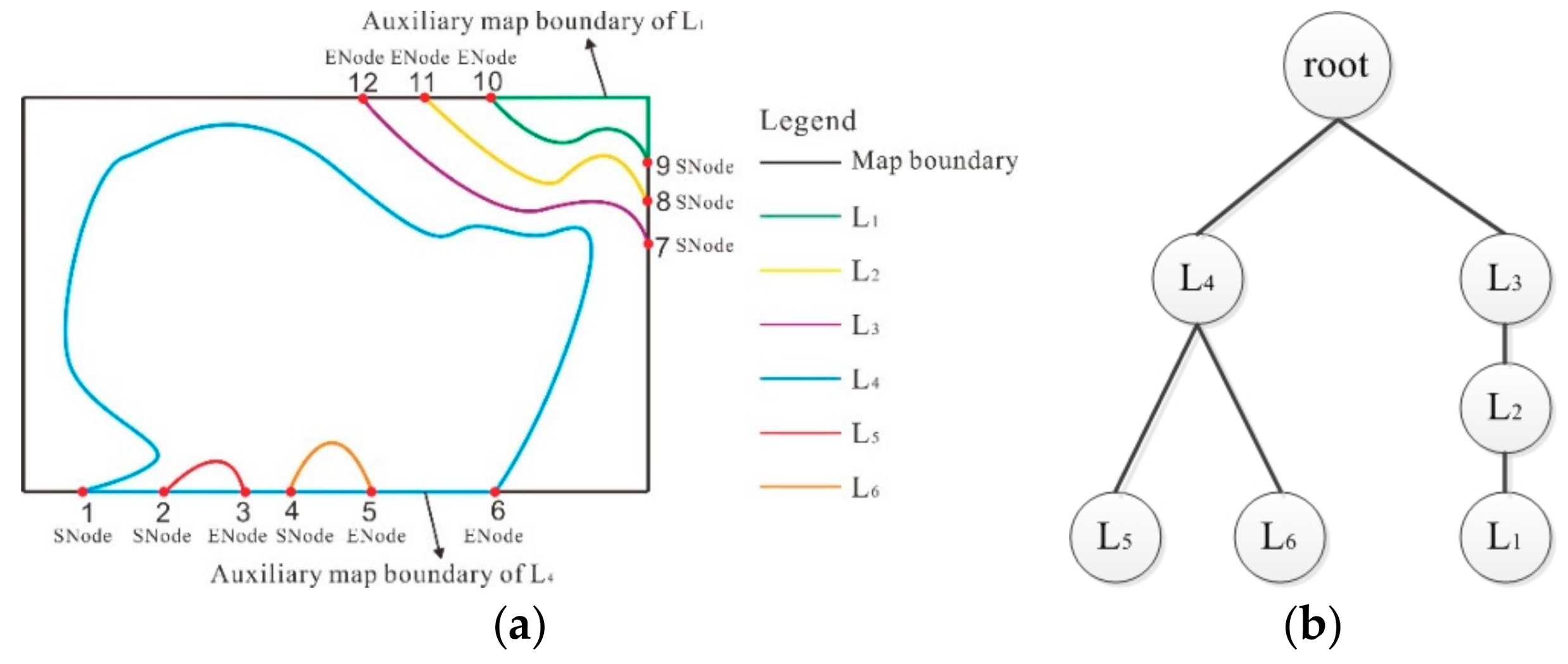
3.2.1. Determination of Adjacent Relation

Generally, an open contour will intersect the boundaries of a map at two points. Hence, we deduce the following rules:
Rule 1: If there are no contour intersections between the two intersections that belong to the same open contour line, then the two intersections are “adjacent” to each other, and the corresponding open contour is denoted a “seed contour”.
Rule 2: A seed contour’s intersections with the map are ordered counterclockwise along the map boundary. Based on this order, these intersections are designated the “starting node” (SNode) and “ending node” (ENode).
Rule 3: The map intersections of non-seed open contours are labeled according to their adjacencies and distance from the intersections of the seed contour. In other words, the map intersection of a non-seed open contour, the nearest node of which is the SNode of a seed contour, is also denoted a SNode. Similarly, the map intersection whose nearest node is the ENode of a seed contour is denoted an ENode.
Rule 4: The portion of the map boundary between a SNode and ENode pair is referred to as the “auxiliary map boundary” of the open contour.
Defining the bottom left corner point of the map boundary as the origin, the distances are calculated between each intersection and the origin point moving counterclockwise around the map boundary. These intersections are then labeled 1, 2, 3, …, n, in ascending order of their distance from the origin.
As depicted in Figure 3a, contours L1L6 are open contours, with L1, L5, and L6 being seed contours. Points 9, 2, and 4 are the SNodes of L1, L4, and L5, whereas points 10, 3, and 5 are the ENodes of L1, L5, and L6, respectively.
The adjacent relation of open contours may then be treated as the determination of the adjacent relation between each intersection, as defined in the following: If an adjacent relation exists between S N o d e L i and S N o d e L j , E N o d e L i and E N o d e L j , and the auxiliary map boundary of Li is a part of the auxiliary map boundary of Lj, then Li, and Lj are adjacent to each other, with Li being internally adjacent to Lj, while Lj is externally adjacent to Li. If adjacencies are present between S N o d e L i and S N o d e L j (or E N o d e L j ) and between E N o d e L i and S N o d e L j (or E N o d e L j ), and there is no overlap between their auxiliary map boundaries, then Li and Lj are denoted parallel-adjacent.

3.2.2. Branched Tree of Open Contours

First, an arbitrary seed contour is selected as the initial contour, such as L1 in Figure 3a. The contours are then ordered and marked according to the distances between their boundary intersections and the origin, the bottom left corner of the map, to determine the adjacent contours of the initial contour. As demonstrated in Figure 3a,b, L2 is the externally adjacent contour of L1, and L3 is parallel-adjacent to L4. An “outwards” search for adjacent contours is then iterated continuously until all contours have been processed. The definitions of parent nodes and sub-nodes are the same as those implemented in the closed-contour adjacent relation tree. Figure 3a represents a simple case of open contours, which Figure 3b interprets as an adjacent relation tree.

3.3. Merging of Branched Tree and Direction Adjustments

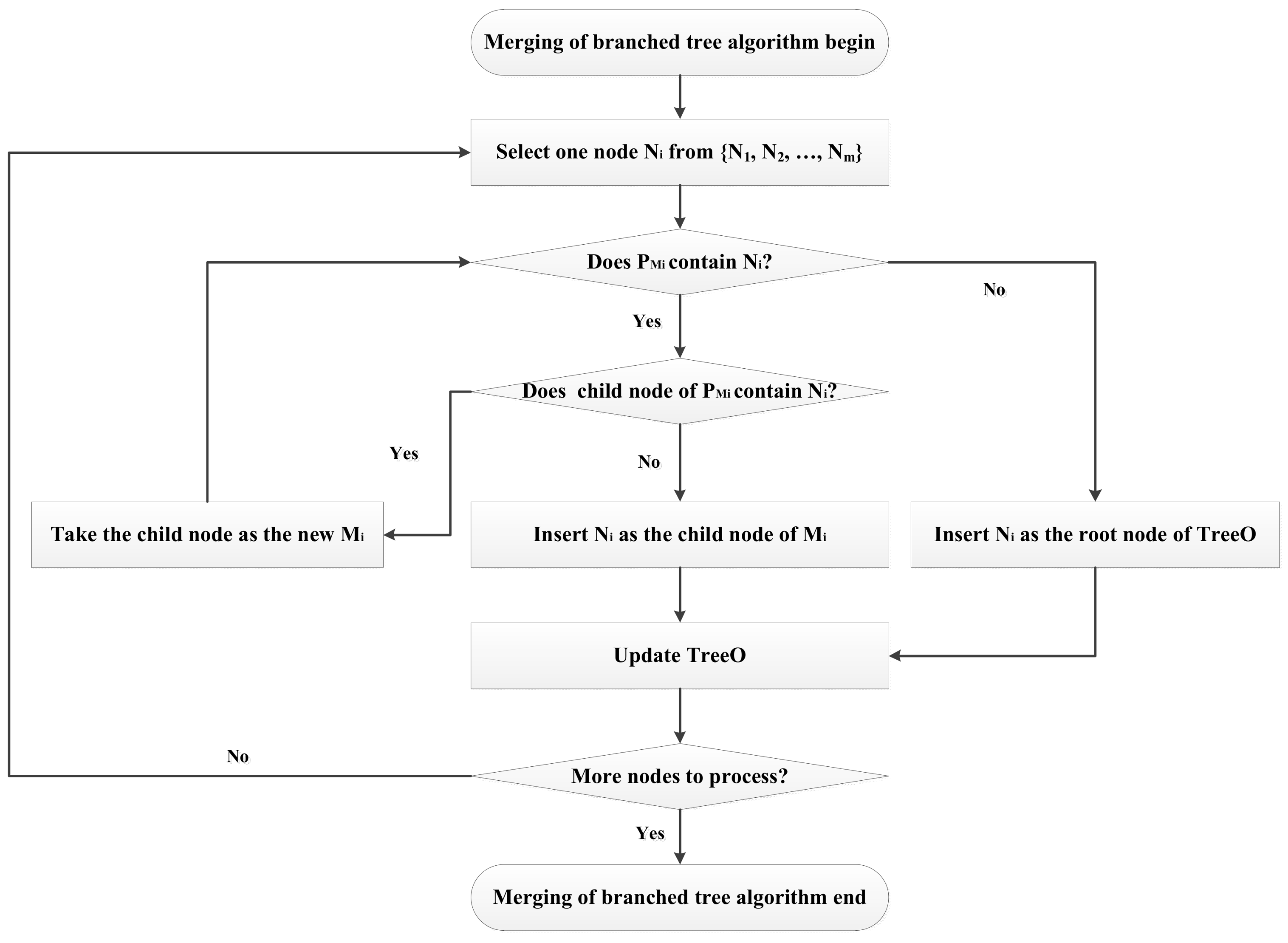
3.3.1. Merging of Branched Tree

Because maps usually comprise both closed and open contours, it is necessary to merge the branched tree structures of both types of contours. Since a closed contour cannot contain an open contour, in the branches of the closed-contour tree, each child node of the root node and its descending child nodes are wholly “inserted” into the open-contour tree. The position of the insertion is determined by the presence of internal or external adjacencies between the closed surfaces formed by the contours.
Suppose that the child nodes of the root node for a closed-contour adjacent relation tree are {N1, N2, …, Nm} and the child nodes of the root node for an open-contour adjacent relation tree are {M1, M2, …, Mn}. We first perform assisted closure on the open contours to form “pseudo-closed surfaces”. These pseudo-closed surfaces refer to closed areas formed by auxiliary map boundaries and open contours and are expressed as {PM1, PM2, …, PMn}. The algorithm for merging the closed-contour tree (TreeC) and open-contour tree (TreeO) is shown in Figure 4.
To summarize the algorithm, if Ni, which is the child node of the root node in TreeC, does not lie within any pseudo-closed area PMi in TreeO, then Ni is inserted as the child node of root node in TreeO. In contrast, if Ni is located within the pseudo-closed area PMi but not within the pseudo-closed area of any child node of Mi, then Ni is inserted as the child node of Mi.
Figure 5a shows the complete structure of the contours shown in Figure 2a and Figure 3a, where N4 is the singular child node representing the root node of the closed contours. Moving outward from N4, we identify the node with the smallest pseudo-closed surface that contains N4; in this case, the node is M4. Because N4 is not enclosed by the pseudo-closed surfaces of the child nodes of M4, the contour tree below the N4 node is inserted into the open-contour adjacent relation tree as a child node of M4, as shown in Figure 5b.

3.3.2. Direction Adjustments

The direction of a contour can be determined as follows: When moving along the contour line in a given direction, high and low elevation values should lie to the left and right of the line, respectively. Consequently, positive landforms of closed contours should be presented counterclockwise, and the negative landforms should be presented clockwise. The elevation values of nested contours should be equal or exhibit an arithmetic decline between vertical intervals from the inner layers to the outer layers. Therefore, the determination and reconciliation of contour directions can be realized by assigning contour directions according to the adjacent relation tree. Owing to the nesting properties and vertical interval consistency of the contours, the process of assigning contour direction would begin at the leaf nodes of the tree, at the innermost contour with the highest elevation on the map.

Principle for the Determination of Contour Direction

For positive landforms, the basic principles of contour direction adjustments are as follows:
Counterclockwise closed surfaces, or pseudo-closed surfaces, formed by contours with high elevations will be contained by the counterclockwise closed surfaces, or pseudo-closed surfaces, of contours with low elevations. Counterclockwise closed surfaces (or pseudo-closed surfaces) formed by contours with the same elevation will not contain each other.
Hence, we designed an Automatic Contour Direction Adjustment Method (ACDAM), which may be functionally expressed as follows:
A C D A M = F A ( M C o n t o u r , F C o n t o u r , N C o n t o u r )
where FA refers to the automatic adjustment function; MContour is the set of maximum elevation contours, i.e., the contour or contours with the highest elevation in the map area; FContour refers to a previous set of contours whose directions have already been adjusted and initially occur as a null value; NContour refers to the next set of contours for direction adjustment, and the initial value of NContour is the adjacent contours of the maximum elevation contours identified by MContour.

Direction Adjustment for the Set of Maximum Elevation Contours (MContour)

If a map only has a single maximum elevation contour, which is an open contour, this contour is a seed contour. However, the direction of its closure cannot be determined if there are no adjacent contours. This scenario is usually overlooked, as it is relatively uncommon.
If there are multiple maximum elevation contour lines and some, or all, of these contours are open contours, based on the known characteristics of positive landforms, maximum-elevation open contours must be located in the innermost section of the region’s contours. Hence, maximum-elevation open contours must be seed contours. The direction of closure of these contours is counterclockwise around the pseudo-closed surface formed by the open contour and its auxiliary map boundaries.
After the directions of the maximum elevation contours have been determined, we then select an arbitrary maximum elevation contour from which to begin to deduce the directions of other contours, moving from the innermost contour to outermost contour on the map or moving from leaf node to root on the adjacent relation tree.

Adjusting the Direction of Adjacent Contours

Three possible scenarios for the adjacent contours of a contour may be inferred because of the characteristics of contours:
(1)
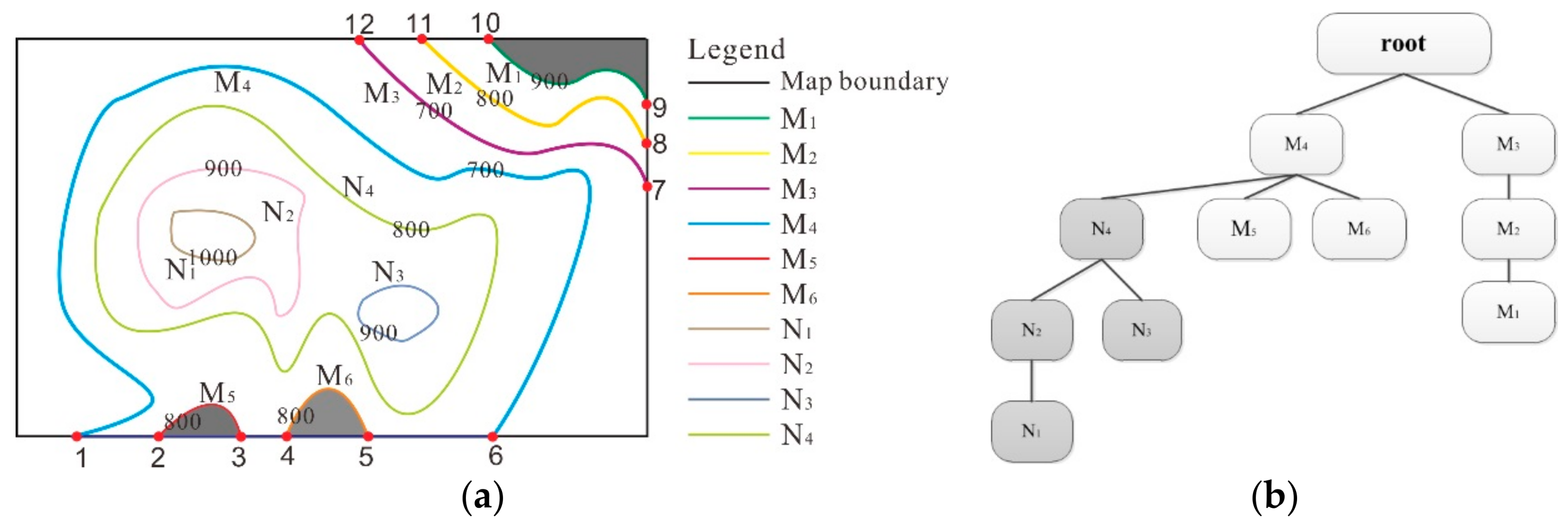
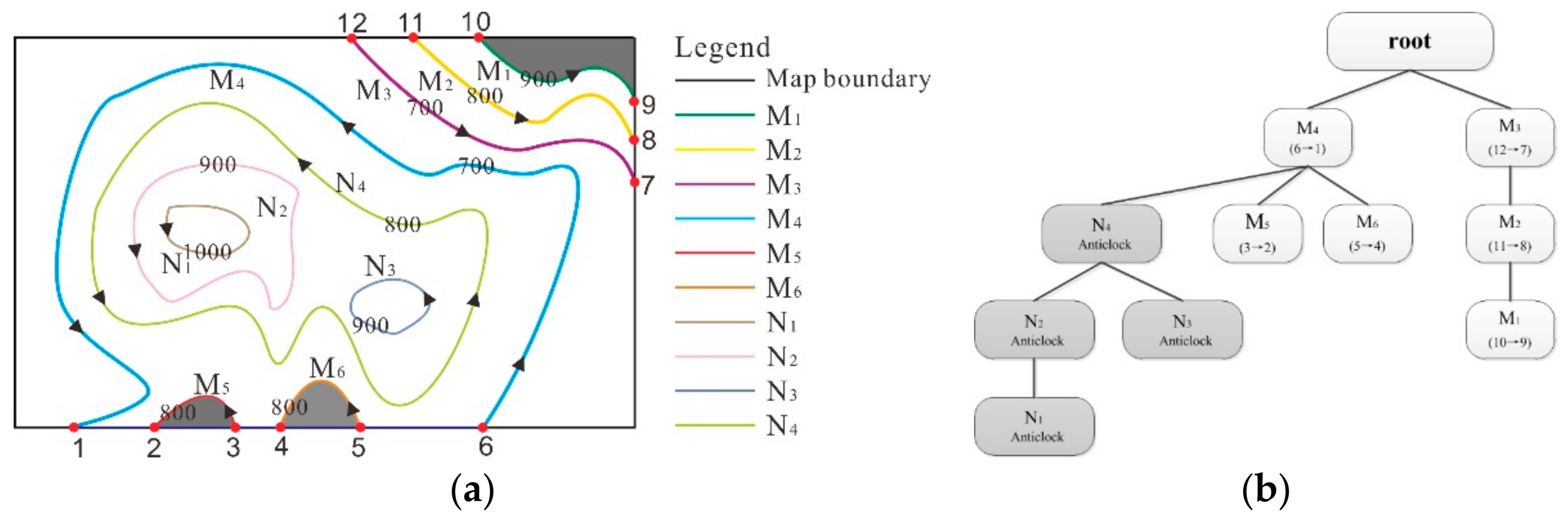
Direction adjustment for adjacent open contours with the same elevation: If an elevational relationship such that NContour = FContour exists, then the adjacent contours have the same elevation. If these contours are open contours, the method for adjusting their direction is as follows: A counterclockwise pseudo-closed surface is formed for the open contour. The open contour’s direction of closure is reversed if an inclusion relationship exists between the closed surface of FContour and the pseudo-closed surface. Figure 6a shows that after processing closed contour N4, its adjacent contours are represented by the parent and sibling nodes depicted in the adjacent contour tree created in Figure 5b. Hence, M4, M5, and M6 are taken as NContour. Note that M5 and M6 have the same elevation as N4, i.e., 800 m, and the counterclockwise pseudo-closed surfaces formed by these contours, as indicated by the darkened regions in Figure 6a, do not overlap with the closed surface enveloped by N4. Hence, the current counterclockwise direction of M5 and M6 is their direction of closure.
(2)
Direction adjustment for adjacent open contours with lower elevations: If an elevational relationship such that NContour < FContour exists, then the adjacent contours have lower elevations. If these contours are open contours, the method for adjusting direction is as follows: A counterclockwise pseudo-closed surface is formed for the open contour. If an inclusion relationship exists between the pseudo-closed surface and the closed surface formed by FContour, the direction of the contour does not require adjustment. Otherwise, the contour’s direction is reversed. In Figure 6a, M4, which is adjacent to N4, has a lower elevation than N4, i.e., 700 m versus 800 m, respectively. Because the pseudo-closed surface of M4 encloses the closed surface of N4, the initially counterclockwise direction of M4 is confirmed as its direction of closure.
(3)
Direction adjustment for adjacent open contours with higher elevations: If an elevational relationship such that NContour > FContour exists, the adjacent contour has a higher elevation. If these contours are open contours, the method for adjusting direction of closure is as follows: A counterclockwise pseudo-closed surface is formed for the open contour. If an inclusion relationship is present between the closed surface of FContour and the pseudo-closed surface, the direction of NContour is reversed. Otherwise, no further processing is required. In Figure 6a, once M3, whose elevation is 700 m, has been processed, its adjacent contour, M2, is selected as NContour, and the elevation of M2 is 800 m. Because the pseudo-closed surface of M2 is contained in the pseudo-closed surface of M3, the initially counterclockwise direction is confirmed as the direction of closure of M2.
By extending the directional information of the “directed contour lines” on the map in Figure 6a to the adjacent relation tree, the DART is obtained, as delineated in Figure 6b. Note that the directions of open contour lines are described according to their SNode-to-ENode directions, whereas the directions of closed contours are described as either counterclockwise or clockwise.

4. Terrain Feature Line Extraction Based on DART

In this section, valley lines are extracted using the terrain feature line extraction method based on DART. To identify valley feature points located downward from a maximum elevation contour, one must search among the adjacent contours of the maximum elevation contour [30,31]. In this paper, the search range is significantly narrowed by the existence of a DART.

4.1. Feature Point Detection and Connection

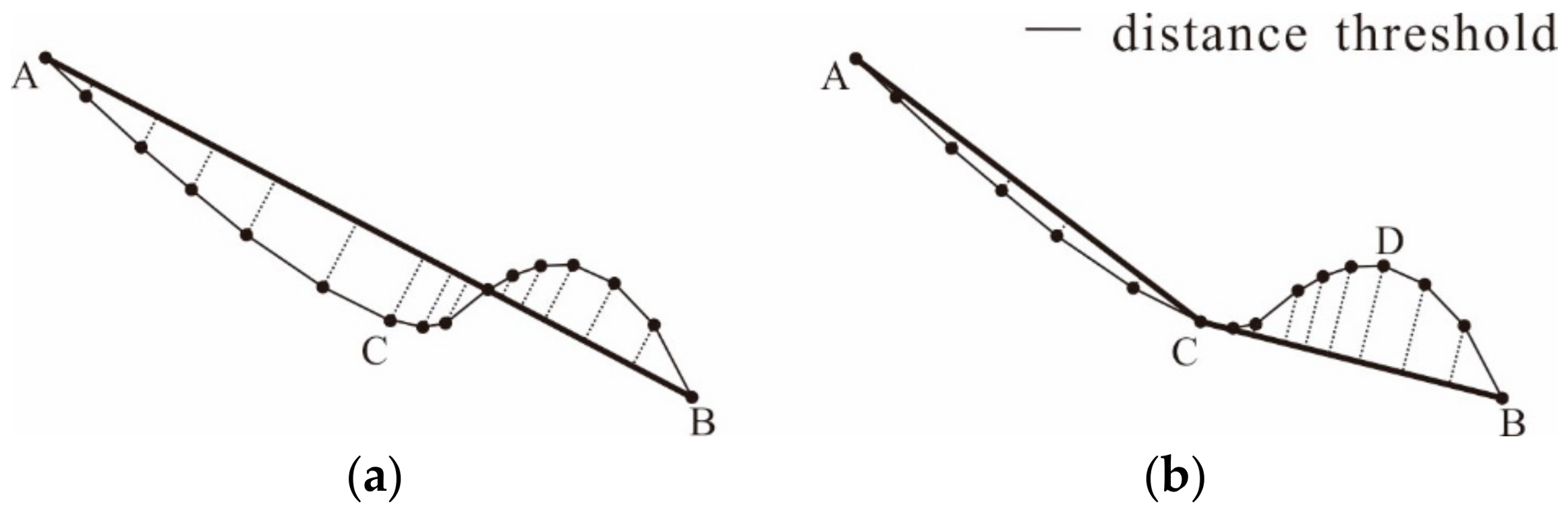
4.1.1. D–P Algorithm-Based Feature Point Detection

It is possible to achieve high levels of accuracy in feature point detection using currently available contour curvature-based methods of detection. However, the features of neighboring curves can interfere with each other. Therefore, we chose to use the D–P algorithm to extract contour feature points. The D–P algorithm is a classic line simplification algorithm. The basic principle of this algorithm addresses the interference issue by setting distance thresholds to detect the feature points of a curve. Figure 7 illustrates the results of the calculations of the D–P algorithm on L2 in Figure 3.
The first step of the D–P algorithm is to detect the point on the curve the distance of which from the line connecting the start and end nodes of the curve is maximal and meets the distance threshold. This procedure detects feature point C in the first step, as depicted in Figure 7a. Feature point C is then used as a segmentation node. In Figure 7b, feature point D is obtained by repeating the previous process on the BC line segment. The distance threshold value, which is usually an empirical value, directly affects the identification of feature points by the D–P algorithm. In this paper, the threshold value was determined by the contour interval of the original data. That is, the distance threshold is equal to the contour interval or a multiple of the contour interval.
For the directed L2 curve, the vector cross-product method [32] can be used to determine the convexity or concavity of each feature point according to the counterclockwise direction of the contours. When the direction of the curve is counterclockwise, if the cross-product result of P i 1 P i and P i P i + 1 for point Pi is positive, Pi is convex point. However, if the result is negative, Pi is a concave point, as indicated by the blue and red points in Figure 8. The feature points are then tracked as sets of either convex or concave points and connected to each other to form ridge and valley lines, respectively. Figure 8 displays the output of this process, with the ridge line shown in blue and the valley line in red, corresponding to the colors identifying the individual feature points as convex and concave [33,34].

4.1.2. Connection of Feature Points

The connection of feature points is the process of connecting ridge or valley feature points to form terrain feature lines. Feature points on adjacent contour lines are matched according to the following principles:
(1)
The principle of closest distance: it is likely that the two closest feature points on adjacent contours can be connected to form a terrain feature line.
(2)
The principle of natural extension: feature points on adjacent contours that naturally extend along the advancing trend are most likely to be connected to form a terrain feature line.
(3)
The non-crossing principle: the connection of feature points on adjacent contours cannot cross a contour or other pre-existing terrain feature lines.
The principles of closest distance and natural extension are used to connect feature points that are spatially adjacent and extendable into lines. The non-crossing principle is used to eliminate unreasonable feature point connections.
In this study, the tracking and connection of terrain feature lines were based on the directed adjacent relation tree. To improve the accuracy of the extension direction of each terrain feature line, valley lines were tracked starting from the root node of the adjacent relation tree, which represents the contour with the lowest elevation, and moving out along the branches to the leaf nodes of the DART. In contrast, ridge lines were tracked starting from the leaf nodes, which represent the maximum elevation contours, and moving along the branches to the root of the DART.

4.2. Integrity Compensation for Terrain Features

Although line feature extraction using the D–P algorithm will not lead to the extraction of redundant feature points at each terrain feature segment, a small number of curvature features are sometimes overlooked during extraction using this algorithm. Hence, the connection of feature points using the aforementioned principles can lead to local discontinuities in the terrain feature lines. To address this issue, we propose a “slope extension method” to perform integrity compensation on terrain feature lines. Drawn from the directed adjacent relation tree, the essential idea of this algorithm is as follows: When calculating the direction of slope extension for each valley line, the initial direction is determined by the direction between the two feature points in the maximum elevation contour and its adjacent contour. Then, the valley line is extended toward the contour with lower elevation. If the branch valley line intersects with a main valley line after being extended to a predetermined range, the compensation of the valley line is complete. However, if the valley line does not intersect with a main valley line after being extended, this segment of the valley line is left as-is.
After many experiments, we selected the 5th-order adjacent domain, which contains contours that are adjacent within five contours, as the predetermined range. Figure 9a illustrates the original contour data and the valley terrain features extracted from the contours using the D–P algorithm. The feature points were then connected according to the aforementioned matching principles to form the valley feature lines L1, L2, L3, L4, and L5, as shown in Figure 9b. Note that there are discontinuities in the feature lines due to differences in density of the feature point distributions. The proposed slope extension method was used to perform integrity compensations, which lead to the joining of L5 to L4 and the joining of L4 and L2 to L1. L3 was not joined to L1, as the distance between these lines exceeds the 5th-order adjacent domain. The results of integrity compensation are shown in Figure 9c.

5. Experiments and Analysis

To validate the accuracy and efficiency of our methods, our directed adjacent relation tree and method for the extraction of terrain feature lines were embedded within the WJ-III mapping workstation developed by the Chinese Academy of Surveying and Mapping. The visual comparison method was applied to evaluate the accuracy of the terrain feature lines extracted by our method. Cartographic expert knowledge also enabled us to judge the terrain feature lines extracted by the proposed method as complete, continuous, and consistent with the actual terrain. Moreover, to validate the efficiency of our method, we compared the processing time of the approach based on Delaunay triangulation with that of the method proposed in this paper on three sets of contour data.

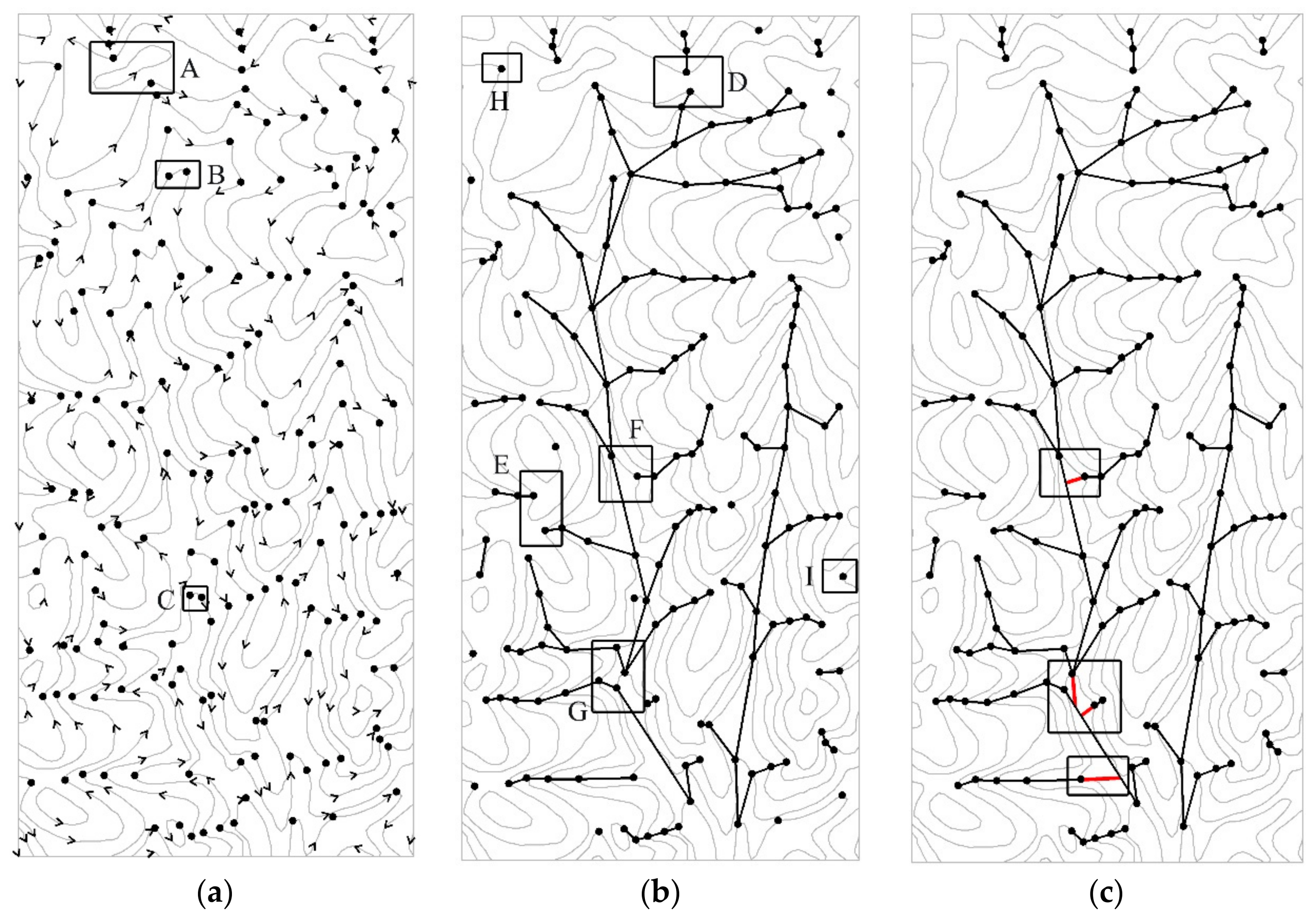
5.1. Experimental Area

An experiment was performed using the contour data of a region in Shanxi Province, which is displayed in Figure 10a. The scale of the experimental dataset is 1:250,000, and the contour interval is 100 m. This region includes a variety of topographic features, such as hilltops, low-lying land, and saddles, and highly complex and varied contour shapes. Furthermore, large numbers of open contours are interrupted by the boundaries of the map. These varied features make the experimental dataset a representative test set for our method.

5.2. Experimental Result and Accuracy Analysis

Figure 10a illustrates the set of valley points obtained by performing direction adjustments according to the DART. The direction of each contour line shows great consistency in Figure 10a, and the ordered arrangement of the valley points on the adjacent contours verifies the accuracy of our method from another perspective. Our method for extracting valley points was not affected by terrain complexity and proved highly effective in contour curvature detection. The terrain feature points were extracted in an exhaustive manner without redundancy. The extracted feature points also exhibit distinct structured features. However, there are weaknesses in our method. The extraction of feature points is significantly affected by the distance threshold values in the D–P algorithm. In this experiment, 100 m was selected as the distance threshold value, consistent with the contour interval of the original data. Rectangle A in Figure 10a depicts the terrain feature points of a hilltop contour that were not extracted successfully because the calculated distance of each point is smaller than the distance threshold. In addition, excessive feature points appeared in segments with high curvatures, as observed in the areas defined by rectangles B and C.
Figure 10b illustrates the valley lines formed by the connection of valley points in Figure 10a. The extracted terrain feature lines in Figure 10b are complete and continuous. The connections of the feature lines in rectangles D and E demonstrate the natural extension and non-crossing principles However, local discontinuities do occur during the connection of features to form feature lines due to differences in density in the feature point distributions, as indicated in rectangles F and G. The single points that cannot form a valley line are deleted, as shown in rectangles H and I in Figure 10b. Figure 10c illustrates the results of performing integrity compensation on the terrain feature lines via the slope extension method proposed in this work. The compensated feature lines form a complete valley line system and provide an excellent overview of the region’s topography.

5.3. Efficiency Analysis

Delaunay triangulation is a geometric structure of computational geometry [35]. The method is widely applied in map generalization and adjacency relation processing owing to its excellent properties, such as proximity, optimality, regionality, and generation of convex polygons [36,37]. Shewchuk [38] proposed the most commonly used method for Delaunay triangulation. We programmed this method based on the TRIANGLE LIBRARY, a Delaunay triangulation library developed by Shewchuk’s research group, and packaged it into the WJ-III mapping workstation. The processing times of this approach were then compared with those of the proposed method to evaluate efficiency.
Delaunay triangulation and the methods proposed in this work were used to process three sets of contour data, which covered larger areas than did the previous dataset. The relationship table of the pairwise adjacencies between all contours in the area was used as a target for validating the efficiency of our method in determining contour adjacencies. The conditions of each dataset and the corresponding processing times of each method are detailed in Table 1. When the area of the dataset was approximately 1000 km2, the efficiencies of our method and Delaunay triangulation in the determination of contour adjacencies were similar, as evidenced by the short processing times achieved by both methods. When the area of the dataset was increased to 5000 km2, the number of contours was more than doubled, and the number of processing points was increased by a factor of 4.36 over the 1000 km2 dataset. The time required by our method to determine contour adjacencies increased by only 0.392 s and was thus insignificant, whereas the processing time for Delaunay triangulation increased by 13 s due to the increase in the number of processing points. When the area of the dataset was increased to 15,000 km2, the time required for the judgment of contour adjacencies by Delaunay triangulation was more than one minute, nearly 11 times as long as the processing time of our method. Hence, our method demonstrates significantly higher efficiency than does Delaunay triangulation when processing large contour datasets.

6. Concluding Remarks

The extraction of terrain feature lines from contours in an automated, efficient, and rational manner has posed a persistent challenge for topographic research. Key aspects of this problem are the detection of contour adjacencies and contour direction determinations for both closed and open contours within map. As currently available methods for terrain feature line extraction are either inefficient or inaccurate, we proposed a method for terrain feature line extraction based on directed adjacent relation trees. In our method, the first step is to construct a directed adjacent relation tree. The classic D–P algorithm is then used to extract terrain feature points. Valley and ridge points are identified accurately from the extracted points and connected to form terrain feature lines. The slope extension method is then applied to perform integrity compensations on these terrain feature lines. Integrity compensation mitigates the major weaknesses of the D–P algorithm, specifically its inability to form terrain feature lines in areas of local discontinuities due to the lack of terrain feature points. The results of the experiment demonstrate that our method is more efficient than conventional methods and produces terrain feature lines that are complete, continuous, and consistent with actual terrain. The superior performance of our method demonstrated in this study indicates that it is highly suitable for a wide range of applications.
Nonetheless, there is room for improvement in our method. The first weakness is the method’s focus on the contours of unidirectional landforms. Our method is unable to account for uncommon scenarios with complex combinations of positive and negative landforms. If these scenarios are encountered, we suggest first distinguishing negative from positive landforms. The basic idea of this process is as follows: If the closed surface of a contour with low elevation is contained by a closed surface with higher elevation, then the contour is a negative landform. However, if the closed surface of a contour with high elevation is contained by a closed surface with lower elevation, then the counter is a positive landform. The second weakness of our method is that the identification of feature points is extremely sensitive to the threshold value selected for the D–P algorithm. A feature point will not be identified if the threshold is too large, whereas redundant feature points will be extracted if the threshold is too small. Therefore, further research on the selection of threshold values in different regions and topographies must be performed.

Author Contributions

Chengming Li conceived the original idea for the study. All co-authors conceived and designed the methodology. Peipei Guo was responsible for the processing and analysis of the data. Chengming Li, Xiaoli Liu, and Pengda Wu drafted the manuscript. All authors read and approved the final manuscript.

Acknowledgments

The research was funded by the project supported by the National Key Research and Development Program of China (Grant No. 2016YFF0201305). We are grateful to the National Geomatics Center of China for providing data.

Conflicts of Interest

The authors declare no conflict of interest.

References

  1. Price, C.V.; Wolock, D.M.; Ayers, M.A. Extraction of terrain features from digital elevation models. In Proceedings of the 1989 National Conference Hydraulic, New Orleans, LA, USA, 14–18 August 1989; ASCE: New York, NY, USA, 1989; pp. 845–850. [Google Scholar]
  2. Xie, J. Implementation and performance optimization of a parallel contour line generation algorithm. Comput. Geosci. 2012, 49, 21–28. [Google Scholar] [CrossRef]
  3. Schmieder, A.; Huber, R. Automatic Generation of Contour Lines for Topographic Maps by Means of Airborne High-Resolution Interferometric Radar Data. In Proceedings of the ASPRS Annual Conference, Washington, DC, USA, 22–26 May 2000. [Google Scholar]
  4. Li, Z.; Sui, H.; Gong, J. A system for automated generalization of contour lines. In Proceedings of the International Carthographic Conference, Ottawa, ON, Canada, 14–21 August 1999. [Google Scholar]
  5. O’Callaghan, J.F.; Mark, D.M. The extraction of drainage networks from digital elevation data. Comput. Vis. Graph. Image Process. 1984, 28, 323–344. [Google Scholar] [CrossRef]
  6. Metz, M.; Mitasova, H.; Harmon, R.S. Efficient extraction of drainage networks from massive, radar-based elevation models with least cost path search. Hydrol. Earth Syst. Sci. 2011, 15, 667–678. [Google Scholar] [CrossRef]
  7. Gong, J.; Xie, J. Extraction of drainage networks from large terrain datasets using high throughput computing. Comput. Geosci. 2009, 35, 337–346. [Google Scholar] [CrossRef]
  8. Zhu, Q.; Tian, Y.; Zhao, J. An efficient depression processing algorithm for hydrologic analysis. Comput. Geosci. 2006, 32, 615–623. [Google Scholar] [CrossRef]
  9. Yoeli, P. Computer-assisted determination of the valley and ridge lines of digital terrain models. Int. Yearbook Cartogr. 1984, 24, 197–206. [Google Scholar]
  10. Jenson, S.K.; Domingue, J.O. Extracting Topographic Structure from Digital Elevation Data for Geographic Information System Analysis. Photogramm. Eng. Remote Sens. 1988, 54, 1593–1600. [Google Scholar]
  11. Zhang, Y.; Fan, H.; Li, Y. A Method of Terrian Feature Extraction Based on Contour. Acta Geod. Cartogr. Sin. 2013, 42, 574–580. [Google Scholar]
  12. Li, Z.; Sui, H. An integrated technique for automated generalization of contour maps. Cartogr. J. 2000, 37, 29–37. [Google Scholar] [CrossRef]
  13. Cronin, T. Classifying Hills and Valleys in Digitized Terrain. Photogramm. Eng. Remote Sens. 2000, 66, 1129–1137. [Google Scholar]
  14. Carr, H.; Snoeyink, J. Representing interpolant topology for contour tree computation. In Topology-Based Methods in Visualization II; Hege, H.-C., Polthier, K., Scheuermann, G., Eds.; Springer: Berlin/Heidelberg, Germany, 2009; pp. 59–73. [Google Scholar]
  15. Pascucci, V.; Cole-McLaughlin, K.; Scorzelli, G. Multi-resolution computation and presentation of contour trees. In Proceedings of the IASTED Conference on Visualization, Imaging, and Image, Marbella, Spain, 6–8 September 2004. [Google Scholar]
  16. Qiao, C.F.; Chen, J.; Zhao, R.L. Preliminary studies on contour tree-based topographic data mining. In Proceedings of the International Symposium on Spatio-Temporal, Beijing, China, 27–29 Aug 2005. [Google Scholar]
  17. Poorten, P.; Jones, C.B. Customisable line generalization using Delaunay triangulation CD-Rom. In Proceedings of the 19th International Cartographic Association Conference, Ottawa, ON, Canada, 14–21 August 1999; Volume 8. [Google Scholar]
  18. Zhang, Y.; Fan, H.; Huang, W. The Method of Generating Contour Tree Based on Contour Delaunay Triangulation. Acta Geod. Cartogr. Sin. 2012, 41, 461–474. [Google Scholar]
  19. Roubal, J.; Poiker, T.K. Automated Contour Labelling and the Contour Tree. Proc. AUTO-CARTO 1985, 7, 472–481. [Google Scholar]
  20. Douglas, D.H.; Peucker, T.K. Algorithms for the reduction of the number of points required to represent a digitized line or caricature. Can. Cartogr. 1973, 10, 112–122. [Google Scholar] [CrossRef]
  21. Gökgöz, T.; Selçuk, M. A New Approach for the Simplification of Contours. Cartographica 2004, 39, 37–44. [Google Scholar] [CrossRef]
  22. Guo, X.; Li, R.; Huang, C. Direction difference in terrain features extraction. In Proceedings of the International Symposium on Spatial Analysis, Spatial-Temporal Data Modeling, and Data Mining, Wuhan, China, 13–14 October 2009; Volume 7492, p. 749243. [Google Scholar]
  23. Song, Y.; Shan, J. An Adaptive Approach to Topographic Feature Extraction from Digital Terrain Models. Photogramm. Eng. Remote Sens. 2009, 75, 281–290. [Google Scholar] [CrossRef]
  24. Liu, H.J.; Jin, H.L.; Miao, B.L. An Algorithm for Extracting Terrain Structure Lines Based on Contour Data. In Proceedings of the SPIE–The International Symposium on Digital Earth: Models, Algorithms, and Virtual Reality, International Society for Optics and Photonics, Beijing, China, 4 November 2010. [Google Scholar]
  25. Ai, T.H. The Drainage Network Extraction from Contour Lines for Contour Line Generalization. ISPRS J. Photogramm. Remote Sens. 2007, 62, 93–103. [Google Scholar] [CrossRef]
  26. Zhang, C.; Zhang, X.; Jiang, W. Rule-based Extraction of Spatial Relations in Natural Language Text. In Proceedings of the International Conference on Computational Intelligence and Software Engineering, CiSE 2009, Wuhan, China, 11–13 December 2009; IEEE: Wuhan, China, 2009; pp. 1–4. [Google Scholar]
  27. Palomar-Vázquez, J.; Pardo-Pascual, J. Automated spot heights generalisation in trail maps. Int. J. Geogr. Inf. Sci. 2008, 22, 91–110. [Google Scholar] [CrossRef]
  28. Carr, H.; Snoeyink, J.; Van De Panne, M. Flexible isosurfaces: Simplifying and displaying scalar topology using the contour tree. Comput. Geom. 2010, 43, 42–58. [Google Scholar] [CrossRef]
  29. Acharya, A.; Natarajan, V. A parallel and memory efficient algorithm for constructing the contour tree. In Proceedings of the 2015 IEEE Pacific Visualization Symposium (PacificVis), Hangzhou, China, 14–17 April 2015; pp. 271–278. [Google Scholar]
  30. Gilperez, A.; Alonso-Fernandez, F.; Pecharroman, S. Off-line signature verification using contour features. In Proceedings of the 11th International Conference on Frontiers in Handwriting Recognition, Montréal, QC, Canada, 19–21 August 2008; CENPARMI, Concordia University: Montréal, QC, Canada, 2008. [Google Scholar]
  31. Zhou, J.; Takatsuka, M. Automatic transfer function generation using contour tree controlled residue flow model and color harmonics. IEEE Trans. Vis. Comput. Gragph. 2009, 15, 1481–1488. [Google Scholar] [CrossRef] [PubMed]
  32. Wong, K.T.; Yuan, X. “Vector Cross-Product Direction-Finding” with an Electromagnetic Vector-Sensor of Six Orthogonally Oriented But Spatially Noncollocating Dipoles/Loops. IEEE Trans. Signal Process. 2010, 59, 160–171. [Google Scholar] [CrossRef]
  33. Ai, T.; Li, J. A DEM generalization by minor valley branch detection and grid filling. ISPRS J. Photogramm. Remote Sens. 2010, 65, 198–207. [Google Scholar] [CrossRef]
  34. Kweon, I.S.; Kanade, T. Extracting topographic terrain features from elevation maps. CVGIP Image Understand. 1994, 59, 171–182. [Google Scholar] [CrossRef]
  35. Zhang, X.; Zhang, C.; Du, C. SVM based extraction of spatial relations in text. In Proceedings of the IEEE International Conference on Spatial Data Mining and Geographical Knowledge Services, Fuzhou, China, 29 June–1 July 2011; IEEE: Piscataway, NJ, USA, 2011; pp. 529–533. [Google Scholar]
  36. Ruas, A. Multiple Paradigms for Automating Map Generalization: Geometry, Topology, Hierarchical Partitioning and Local Triangulation. In Proceedings of the ACSM/ASPRS Annual Convention and Exposition, Washington, DC, USA, 27 February–2 March 1995; pp. 69–78. [Google Scholar]
  37. Ware, J.M.; Jones, C.B.; Bundy, G.L. A Triangulated Spatial Model for Cartographic Generalization of Areal Objects. In Proceedings of the International Conference on Spatial Information Theory, Vienna, Austria, 21–23 September 1995; Taylor & Francis: London, UK, 1997; pp. 173–192. [Google Scholar]
  38. Shewchuk, J.R. Delaunay refinement algorithms for triangular mesh generation. Comput. Geom. Theory Appl. 2014, 47, 741–778. [Google Scholar] [CrossRef]
Figure 1. Framework of the proposed method.
Ijgi 07 00163 g001
Figure 2. An adjacent relation tree for closed contours: (a) closed contour lines and (b) adjacent relation tree.
Ijgi 07 00163 g002
Figure 3. An adjacent relation tree of open contours: (a) open contour lines and (b) adjacent relation tree.
Ijgi 07 00163 g003
Figure 4. Flow diagram of merging of branched tree algorithm.
Ijgi 07 00163 g004
Figure 5. Merging of open- and closed-contour adjacent relation trees: (a) complete structure of the contour lines in the area and (b) unified adjacent relation tree.
Ijgi 07 00163 g005
Figure 6. Automatic direction adjustment of contour direction: (a) contour lines labeled with elevation and direction and (b) “directed adjacent relation tree” (DART).
Ijgi 07 00163 g006
Figure 7. Extraction of terrain feature points based on the D–P algorithm: (a) feature point C is derived from start and end nodes A and B and (b) feature point D is derived from segment BC.
Ijgi 07 00163 g007
Figure 8. Identification of concave or convex points.
Ijgi 07 00163 g008
Figure 9. Connection of terrain feature lines: (a) terrain feature points, (b) terrain feature lines, and (c) compensation of terrain feature lines.
Ijgi 07 00163 g009
Figure 10. Comparison between the valley points extracted before and after contour direction adjustments: (a) valley points extracted prior to direction adjustment, (b) valley points extracted after direction adjustments, and (c) valley lines compensated by the slope extension method.
Ijgi 07 00163 g010
Table 1. Overview of experimental results.
DatasetArea Represented by the Dataset (km2)Number of ContoursNumber of Processing PointsProcessing Time Using Our Method (s)Processing Time Using Delaunay Triangulation (s)
Dataset 11183.2669593,4940.2122.453
Dataset 24996.741528408,1680.60413.235
Dataset 314,609.3742701,150,2395.61661.505

