Abstract
As one of the most popular social networking services in the world, Twitter allows users to post messages along with their current geographic locations. Such georeferenced or geo-tagged Twitter datasets can benefit location-based services, targeted advertising and geosocial studies. Our study focused on the detection of small-scale spatial-temporal events and their textual content. First, we used Spatial-Temporal Density-Based Spatial Clustering of Applications with Noise (ST-DBSCAN) to spatially-temporally cluster the tweets. Then, the word frequencies were summarized for each cluster and the potential topics were modeled by the Latent Dirichlet Allocation (LDA) algorithm. Using two years of Twitter data from four college cities in the U.S., we were able to determine the spatial-temporal patterns of two known events, two unknown events and one recurring event, which then were further explored and modeled to identify the semantic content about the events. This paper presents our process and recommendations for both finding event-related tweets as well as understanding the spatial-temporal behaviors and semantic natures of the detected events.
1. Introduction
Twitter is one of the most popular social networking and microblogging services in the world. Millions of people use it to remain socially connected to their friends, family and co-workers [1]. Twitter users can send short messages, called “tweets,” of up to 140 English language characters. Since 7 November 2017, this limit has doubled to 280 characters. The common practice of responding to a tweet has evolved into a distinct markup culture: “RT” stands for retweet, “@” followed by a user identifier addresses the user and “#” followed by a word represents a hashtag [2]. Launched in 2006, Twitter has rapidly gained popularity worldwide. As of 2017, Twitter had reached 330 million monthly active users [3] and an estimated 500 million tweets are sent per day (http://www.internetlivestats.com/twitter-statistics/). Because these massive Twitter data can be accessed programmatically via APIs, Twitter has been a treasure trove for geo-social researchers based on big data [4], which offers an unprecedented opportunity to study social networks and human communication with active data [5,6], thus making tweets one of the favorite data sources of geo-social researchers [7,8].
Twitter enables users to post tweets with their current locations (longitude and latitude) shared, that is, georeferenced or geo-tagged tweets [9]. With an average rate of 0.85–3% tweets being geo-tagged, around 7,000,000 geo-tagged tweets are posted per day [10,11]. Many crowd-sourced sensing and collaboration projects take advantage of such geographic information [12]; these data have useful implications for human geography, geographic disease and influenza trends, location-based services, targeted advertising and urban science, as well as social network studies [13,14,15]. Tweets have become a promising alternative, or even a better one, to traditional survey data due to the immense volume and diverse information they contain, offering new opportunities for discovering geo-social knowledge and novel research approaches in a variety of fields [8,16].
Geo-tagged tweets open the possibility of detecting real-world events from social media data [17] and infer quantitative information [18]. In addition to knowing who is involved in an event, three other main aspects (3W questions) are important for understanding an event: (1) when did it happen, (2) where did it happen and (3) what happened? A Twitter dataset contains a time-stamp, geo-location and text information, which make it a valuable data source for such research. Compared to traditional survey data, however, it requires proper study methods. It is not easy to collect social media data nor to categorize it. Within one area of interest, there might be hundreds of thousands of active users contributing their tweet datasets and the topics can vary from celebrating a birthday in a restaurant to sharing a sad break-up on a bench in a park. Therefore, identifying distinctive topics within these massive datasets can be difficult.
As shown in Figure 1, by considering different scales related to the number of people involved, spatial distribution, time duration, textual information and so forth, it is possible to classify events into different categories. Events that are well known to the public and attract general attention fall into the large scale (national and state scale) category as they can be studied mostly by textual mining. Examples of typical large-scale events are presidential elections, nationwide policies, or severe disasters. For these events, their locations and times are less important or of interest since they often are widespread and last a reasonably long time. The semantics of events can become more diverse and have higher perplexity as their spatial and temporal domains become larger. This means the content of the tweet messages over a larger area and longer time period would be less focused and clustered. In this study, we focused on small-scale (city and community scale) events that might involve several to tens of people, occur in a neighborhood extending from a community to a city (~kilometers in range) and last from one to several hours. Detecting small-scale events poses difficulties and is of particular interest since they are usually hidden or latent and there is no prior knowledge of when, where and what events may happen.
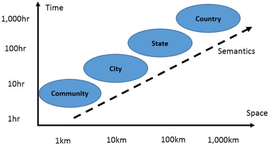
Figure 1.
Dimensions and scales in event detection.
The objective of our study was to discover and understand small-scale events that have happened by using Twitter data. Our work is presented in six sections. The motivation was discussed above (Section 1); Section 2 is a review of the past related work; Section 3 describes the methodology and workflow for spatial-temporal clustering and text analysis; Section 4 describes the Twitter data used for the study and presents the results in spatial, temporal and textual contexts for a number of detected known events, unknown events and recurring events; Section 5 discusses the implementation of the workflow and its parameter settings; and Section 6 summarizes our conclusions and the limitations of our work.
2. Related work
Event detection has long been a research topic of interest [19]. One of the underlying assumptions of event detection is that the usage of related words will increase during an event. Crampton et al. [20] confirmed the feasibility of using geo-referenced social media data in determining events while they are occurring by focusing on one hashtag associated with a riot. They developed a large data analytic system with geo-visualization capability for geo-tagged tweets. In 2010, Phuvipadawat and Murata [21] presented a method for collecting, grouping, ranking and tracking breaking news from Twitter. Lee and Sumiya [22] introduced a real-time geosocial local event detection system to identify local festivals based on modeling and monitoring crowd behaviors with Twitter data. Weng and Lee [23] proposed an event detection method based on the clustering of discrete wavelet signals produced from words generated by Twitter, while Pennacchiotti and Popescu [24] focused on identifying controversial events that provoked public discussions with opposing opinions on Twitter and extracting events and their descriptions from Twitter. Benson et al. [25] presented a novel approach for identifying Twitter messages for concert events with a factor graph model. In contrast, Sakaki et al. [26] exploited tweets to detect specific types of events, such as earthquakes and typhoons, by training a support vector machine (SVM) on a manually-labeled Twitter dataset. In their succeeding work, they incorporated semantics analysis in their event detection system [27]. Using an approach they developed to detect geospatial, real-world events in real time by analyzing the Twitter stream, Walther and Kaisser [28] could tell whether or not clusters of tweets issued temporally and spatially close to each other described the same real-world event. In 2015, Huang and Wong [29] presented a method to model and visualize Twitter users’ mobility patterns with DBSCAN.
To identify events via Twitter, information in three dimensions is crucial: spatial, temporal and semantic or textual. Spatial information is one of the most important dimensions in event detection, for which spatial clustering methods are widely used. The k-means method [30] and the Expectation Maximization (EM) method [31] are clustering methods. k-means aims to partition the data of observations into k clusters and every data point is marked as a part of the cluster with the nearest mean, thereby constructing a prototype of the cluster. EM determines the maximum likelihood or the maximum posterior estimates of the parameters in statistical models. In addition, some density-based methods also are used for spatial clustering. Given a set of points in space, DBSCAN groups the points that are shared with many nearby neighbors, whereas the isolated points that are far away from others become outliers. Variations of DBSCAN include generalized DBSCAN (GDBSCAN) [32], Ordering Points to Identify the Clustering Structure (OPTICS) [33] and SUBspace CLUstering (SUBCLU) [34], among which OPTICS is an important extension of DBSCAN for hierarchical clustering.
In addition to spatial clustering, some past researchers also attempted to combine the analysis of spatial and temporal information. One such implementation was spatial scan statistics [35], which searches spatio-temporal cylinders. When the density of events of the same type is higher than the density of other types, the places where events occur consistently for a significant amount of time are more likely to contain a cluster. Another method is Spatio-Temporal DBSCAN (ST-DBSCAN), which is an extension of the DBSCAN algorithm to handle the clustering of spatio-temporal data. The major improvement of ST-DBSCAN is that it incorporates the time dimension during the clustering process and uses the thresholds to define both the spatial and temporal neighbors.
In addition to examining the spatial pattern and temporal pattern of an event, it is important to understand the content of the event and extract the topics in the tweets. In natural language processing, a topic model is a statistical model that is referred to as a probabilistic topic model, which is used for extracting potential “topics” hidden behind the documents or texts [36]. In the early use of topic modeling, Deerwester et al. [37] presented a method called latent semantic indexing (LSI), which can analyze relationships among a set of documents and the terms they contain by producing a set of concepts. After the emergence of LSI, another method called probabilistic latent semantic indexing (pLSI) was created [38]. Compared to LSI, which derives from linear algebra and downsizes the occurrence tables, pLSI is based on a mixture decomposition procured from a latent class model. Furthermore, Latent Dirichlet Allocation (LDA) was introduced in 2003 [39] and has become one of the most popular topic models currently in use. LDA allows documents to have a mixture of topics. In LDA, each document may be viewed as a mixture of various topics. LDA is similar to pLSI, except that the topic distribution of LDA is assumed to have a Dirichlet prior. Essentially, the LDA model is the Bayesian version of the pLSI model. In practice, LDA is able to produce more reasonable mixtures of topics in a document. Because the LDA model is highly modular and easy to extend, some extensions emerged from LDA. One such approach is the hierarchical LDA (hLDA) [40], where the nested Chinese restaurant process is used to join topics in a hierarchy. Another extension of LDA is the hierarchical Dirichlet process (HDP) [41], which addresses the problem that the number of topics is not an a priori variable and allows topics to be arranged in a hierarchy, the structure of which can be studied from the data.
3. Methodology
To detect small-scale events, the location and time of the tweets is important and of interest [4,9]. Without prior knowledge of the location and time of a potential event, starting with a textual search would lead to many false negative events. Therefore, instead of searching the textual information in the tweets, we clustered the geo-tagged tweets in the spatial-temporal domain first. Such spatial-temporal clustered tweets were then subject to a word frequency summary and topic clustering to understand the semantics of the event. In this way, we avoided the common ambiguity in text mining. More importantly, this approach allowed us to discover unknown events that have certain clustering effects in the spatial-temporal domain without knowing the nature of the events prior to text mining.
For an individual user, the preferred spatial clustering method is DBSCAN. A user’s tweets can be grouped by time, to which DBSCAN [29] is then applied. After this processing, the spatial patterns of an individual user can be pictured by hours (bins in time). DBSCAN was inadequate for event detection in our study because the temporal scales of our events varied and thus a new method named ST-DBSCAN [42] was used. ST-DBSCAN is based on DBSCAN with some marginal extensions and aims in clustering the data with both spatial and temporal dimensions simultaneously.
Besides spatial and temporal information, textual information can help in identifying the content of potential events. Our study used a list of stop words, that is, the most common words in a language, to filter the text and sort the word frequency in descending order. This approach helped us identify the keywords and content structure of every identified spatial-temporal cluster.
3.1. DBSCAN and ST-DBSCAN
DBSCAN is an unsupervised data clustering algorithm [43]. Unlike k-means, which requires providing the number of clusters, DBSCAN does not need the number of clusters to be specified. It also can detect the clusters that are non-linearly separable, which is helpful in analyzing the complex tweeting patterns of different users. DBSCAN is robust to outliers and can detect and remove the noise from clusters, which keeps the data set clean. DBSCAN requires two parameters: the maximum distance between neighbor points (d) and the minimum number of points needed to form a dense region (minPts). DBSCAN classifies the points as core points, reachable points and outliers as follows [43]:
- (1)
- A point p is a core point if at least minPts points are within a distance d (d-neighborhood) of it. These points are considered to be directly reachable from p. No points are directly reachable from a non-core point.
- (2)
- A point q is reachable from p if there is point chain: a path p1, …, pn with p1 = p and pn = q, where each pi+1 is directly reachable from pi.
- (3)
- All points that are not reachable from any other point are outliers.
By grouping the tweets of one single user and using the hour as the unit to apply DBSCAN, the daily patterns of individual users can be identified and depicted in a spatial timeline. Even though DBSCAN can efficiently understand the daily routine of an individual user, detecting general public events is a more complex task. The activity pattern of the general public is unlikely to follow a norm; and most public events, especially emergencies, do not provide many clues for establishing daily routines.
We therefore used ST-DBSCAN to handle the spatial and temporal properties of the Twitter data. Similar to DBSCAN, ST-DBSCAN has a parameter to measure the similarity of spatial value (d1). In order to support non-spatial data, ST-DBSCAN introduces a new parameter to measure the similarity of non-spatial value (d2), such as temporal distance [42]. For example, A(x1, y1, t1) and B(x2, y2, t2) are two points, while x1, y1, x2, y2 are spatial coordinates and t1, t2 are temporal stamps, then d1 and d2 are calculated, respectively and . Figure 2 shows a cluster in three-dimensional space. The core points and edge points form the cluster, while the noise points do not. For the core points, the number of their neighbor points is greater or equal to minPts, while the edge points are not. However, the edges point is a neighbor of at least one of the core points. The noise points are too far away from any of the clusters.
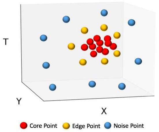
Figure 2.
Spatial-temporal clustering by Spatial-Temporal Density-Based Spatial Clustering of Applications with Noise (ST-DBSCAN).
3.2. Latent Dirichlet Allocation (LDA)
Textual information is another key element of event detection. Without carefully looking at the textual information, it is hard to identify whether there is an actual event happening or only a group of people talking about something meaningless. According to [44], there are mainly two types of topic modeling methods: Probabilistic Latent Semantics Analysis (pLSA) and Latent Dirichlet Allocation (LDA). LDA is an extension of pLSA that introduces a Dirichlet prior on the mixture weights of topics per documents [44,45]. This study used LDA to analyze the textual information in addition to counting word frequency. LDA is a probabilistic framework for modeling the sparse vectors of text data. Its key idea is based on the hypothesis that a group of sentences or a document contains certain topics [45,46]. A topic refers to a group of words having similar or closely related meanings under certain probabilities. A document contains a mixture of different topics. When the author of the document is one person, these topics reflect the individual’s view and vocabulary [46]. In event detection, the topics from LDA refer to the aspects of a particular event.
With the help of LDA, the similarity among the datasets can be explained by grouping the features of the data into unobserved sets. LDA models document D as a mixture over K latent topics and each topic describes a multinomial distribution over a W word vocabulary. Given a bundle of tweets, Figure 3 shows the graphic model representation of the LDA model [39] with Twitter information. In Figure 3:
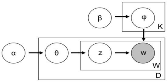
Figure 3.
Graphic model of Latent Dirichlet Allocation (K: Topics, W: Word Vocabulary, D: Document; adapted from Porteous et al. [47].
- α is the parameter of the Dirichlet prior on the document—topic distributions of all tweets
- β is the parameter of the Dirichlet prior on the topic—word distribution of all tweets
- θj is the topic distribution for tweet j
- ϕk is the word distribution for topic k
- zij is the topic for the i-th word in tweet j
- wij is the specific word among all tweets
3.3. Workflow for Event Detection
Based on the principles above, our workflow for event detection was as follows:
- Group tweets by day and generate charts showing the number of tweets and users by the day of the month.
- Apply ST-DBSCAN to cluster the tweets of every day. For every cluster, generate its spatial, temporal and textual patterns.
- Apply LDA to identify potential topics in the cluster and analyze the structure of every tweet. For example, if the probability construction of a sentence is 60% for Topic 1, 40% for Topic 2, then this sentence is labeled as a sentence of Topic 1.
4. Tests and Results
The time span of the data in our study was 1 January 2014 through 31 December 2015. Four U.S. Midwestern college towns were chosen as the study areas: (1) West Lafayette, IN, home of Purdue University; (2) Bloomington, IN, home of Indiana University; (3) Ann Arbor, MI, home of the University of Michigan; and (4) Columbus, OH, home of The Ohio State University [11]. All the Twitter data for research were downloaded through the Twitter streaming application programming interface (API), for which there are three main streaming endpoints [48]:
- (1)
- Public Streams: streams of public data flowing through Twitter can be pushed.
- (2)
- User Streams: streams of a single user, which contain almost all of the data corresponding to the user, can be accessed.
- (3)
- Site Stream: streams of the multi-users version of user streams are accessible.
Because our research objective was to detect events through geo-tagged tweets in the study areas, the public stream method was used with “Tweepy,” a Python library, to conduct the public streaming. The search terms used in the streaming were the coordinate boundaries of the study areas and only the tweets with latitude and longitude information attached, which are usually generated by smartphones with GPS receivers, were included.
4.1. Detection of Known Events
This section provides two examples of detecting known events that occurred.
4.1.1. Gunshot in West Lafayette, IN
The first event happened in January 2014 on the Purdue University West Lafayette, IN campus. The shooting occurred in the Electrical Engineering (EE) building around noon on 21 January 2014 [49]. After the gunshot was heard, people on campus sheltered in place. This sudden and shocking event spread very quickly and people all over West Lafayette, especially students on campus, talked about it on Twitter. During the lock-down period after the gunshot, students checked Twitter for the latest update from Purdue officials as well as their friends and they tweeted or retweeted about the event.
Figure 4a shows the daily pattern during the month of January. It is obvious that the number of tweets on 21 January reached an extreme. According to the temporal pattern in Figure 4b, a “big jump” occurred around 12:00 PM and the discussion was lively between 12:00 PM and 3:30 PM. After that, the discussion kept going with a temperate style until midnight.
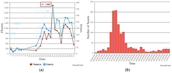
Figure 4.
Number of tweets and users in January 2014 (a) and the hourly pattern on 21 January (b) in West Lafayette.
Figure 5a shows the locations of the spatial-temporal tweet cluster centers determined by ST-DBSCAN on 21 January. These locations are labeled by colored symbols in terms of the number of tweets in each spatial-temporal cluster. As illustrated in Figure 5a, the most significant cluster (the cluster with the most tweets) had 1274 tweets between 9:05 AM and 11:59 PM on that day. The spatial distribution of the tweets within the most significant cluster are marked by the four ovals in Figure 5b. The largest blue oval is the major activity center of Purdue University and the other three ovals represent different residence halls. The scene of the crime, the Electrical Engineering Building, is in the red oval. It did not have the highest frequency of tweets, which reflected that people were concerned for their safety and stayed away from the gunshot location at that time.
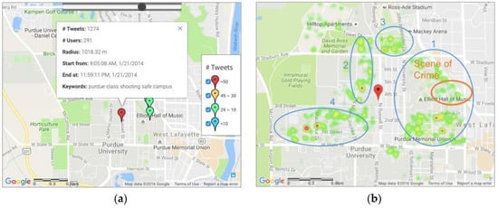
Figure 5.
Spatial-temporal clustering results for the tweets in West Lafayette on 21 January 2014 when the gunshot occurred: (a) cluster centers and the most significant cluster; and (b) distribution of the tweets in the most significant cluster. (d1 = 200 m, d2 = 60 min, minPts = 10).
The word frequency for the most significant cluster is summarized in Table 1. “Purdue” was the hottest word and other words such as “shooting,” “shot,” “police,” and “purdueshooting” showed that the gunshot event spread across the whole campus. Words such as “prayforpurdue,” “love,” “crazy,” and “hope” reflected some of the emotions and attitudes of Twitter users towards this sad event. “EE” stands for Electrical Engineering Building, which was the scene of the crime.

Table 1.
Word frequency of the most significant cluster about the gunshot in West Lafayette, IN.
After the estimation of topic perplexity, six topics were found to be proper for LDA implementation. Table 2 lists the six identified topics (T1 to T6), the top 10 words (W1 to W10) for each topic and the total number of tweets under each topic. The percentage (%) associated with the use of a word refers to the frequency that the word appears in all of the tweets under one topic. Topic 6 had the highest numbers of sentences. Topics 1, 4 and 5 were the topics that contributed most to the keywords “shooting,” “shooter,” and “shot,” which made these topics the most significant indicators of this accident. Topics 3 and 6 both reflected the users’ feelings after the shocking news. Considering the keywords and probabilities of keywords in Topic 2, the topic of normal school life was less related to the event and could be regarded as noise.
Table 2.
Modeled topics of the most significant cluster about the gunshot in West Lafayette, IN.
4.1.2. Saint Patrick’s Day in Columbus, OH
Saint Patrick’s Day is a religious and cultural celebration held on 17 March every year [50]. It is in memory of the well-known patron saint of Ireland [50]. Nowadays, it has become an international festival to celebrate Irish culture through parades, special foods and wearing the color green [50]. On 17 March 2014, there was a great celebration of Saint Patrick’s Day in Columbus, OH including a huge parade across the city. To analyze this event, we accessed the Twitter data from 17 March 2014 to see what it would reveal.
In the first attempt, d1 was chosen as 100 m, d2 as 30 min and minPts as 10. However, we were unable to find any clusters significantly related to Saint Patrick’s Day. A more flexible threshold then was applied; and in this second attempt, we increased d1 to 200 m, while the other parameters remained the same. As a result, the cluster in Figure 6a with a large radius of over 900 m was supposed to be the study cluster. From Figure 6b, it is clear that the event was discussed all over the campus of The Ohio State University and the spatial patterns were not concentrated in one specific location, which may have been due to a significant amount of noise caused by the larger threshold for d1, most of which were normal chats from Twitter users.
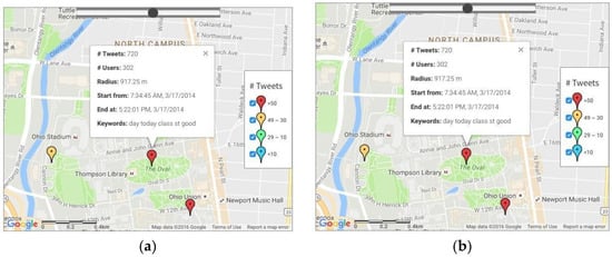
Figure 6.
Spatial-temporal clustering results for tweets on Saint Patrick’s Day, 17 March 2014 in Columbus OH: (a) cluster centers and the most significant cluster; and (b) distribution of the tweets in the most significant cluster.
As shown in Figure 7a, the discussion started in early morning around 8:00 AM and ended around 3:30 PM. In Figure 7b, “Saint” is abbreviated to “St” and “green” refers to the traditional color of the celebration. Because “Patrick” is supposed to appear with “St,” it is surprising that “Patrick” was not in the top 20 words, which may have been due to the fact that people used variations of “Patrick,” such as “Pat,” “Patty,” and “Paddy,” which diluted the actual word frequency. After manually summing up the word frequency of some typical transformations, the word frequency of “Patrick” was 22, which ranked 9th in the word frequency chart.
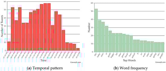
Figure 7.
Temporal pattern and word frequency of Saint Patrick’s Day: (a) Temporal pattern; and (b) Word frequency.
As for topic modeling through LDA, Table 3 shows that only Topics 4 and 5 had some highly related words, such as “wearing,” “green,” “Irish,” “St,” and “Patrick’s,” which could be explained by the fact that people were talking a lot about proper dressing for the holiday. Other topics mostly described the events related to students’ daily activities and were regarded as less relevant.
Table 3.
Modeled topics of the Saint Patrick’s Day in Columbus, OH.
4.2. Detection of Unknown Events
This section discusses the discovery of unknown events without prior knowledge about the event.
4.2.1. Beer Festival in Bloomington
Figure 8 shows a tweet cluster detected on 12 April 2014 in southwest Bloomington. There were some interesting keywords: “beer,” “craft,” “fest,” and “drinking,” which indicated that there might be a beer-drinking event on that date. In Figure 8a, from the scale bar on the heat map, the event talk was quite dense at this location. By reverse-geocoding the cluster center, the event was located near Woolery Stone Mill, which was consistent with the location information in an announcement about the beer festival in Bloom Magazine [51]. For the temporal pattern in Figure 8b, the active period was between 1:30 PM and 6:00 PM, while Bloom Magazine indicated that it happened between 3:00 PM and 7:00 PM. A possible explanation is that some people gathered with their friends before the official opening and people became less active on Twitter at the end of the beer festival.
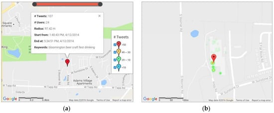
Figure 8.
Spatial-temporal clustering results for tweets about the Bloomington Craft Beer Festival on 12 April 2014: (a) the most significant cluster; and (b) distribution of the tweets in the most significant cluster.
Figure 9 shows that “bloomington,” “beer,” “craft,” “fest,” and “drinking” were the top five words that dominated the word frequency chart, while other words showed a relatively low frequency. The reason for this obvious pattern is that there were two common templates that people used when tweeting. One was “drinking…… @ bloomington craft beer fest,” and the other was “I’m at bloomington craft beer fest (Bloomington, IN) …….” These formatted tweets identified themselves in the structure of the word frequency chart.
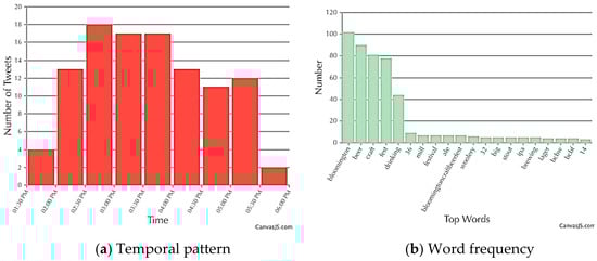
Figure 9.
Temporal pattern and word frequency of the Craft Beer Festival in Bloomington: (a) Temporal pattern; and (b) Word frequency.
With the concentration of topics, rather than using the number of topics with the lowest perplexity, we classified the tweets into two topics with LDA. The results in Table 4 met our expectations and allowed us to identify the topics. The top five words in the word frequency chart all had a high probability in Topic 1; and 83 sentences belonged to Topic 1, while only 25 sentences belonged to Topic 2. In Topic 2, the top word “bloomingtoncraftbeerfest,” a popular hashtag used during the event, was a combination of “bloomington,” “beer,” “craft,” and “fest.”
Table 4.
Modeled topics of Bloomington Craft Beer Festival.
4.2.2. Meryl Streep’s Visit to Indiana University
Figure 10 shows a detected cluster on the Indiana University campus on 16 April 2014. The keywords of this cluster were “merylatiu,” “meryl,” “streep,” “iu,” and “merylstreep.” With the repetitive words, we assumed that the cluster could be related to Meryl Streep, a famous American actress of stage and screen and philanthropist. According to the news [52], on 16 April 2014 Meryl Streep received an honorary doctoral degree and then gave a lecture at the Indiana University Auditorium. According to the pattern in Figure 10, this event was widely spread around the Indiana University Auditorium.
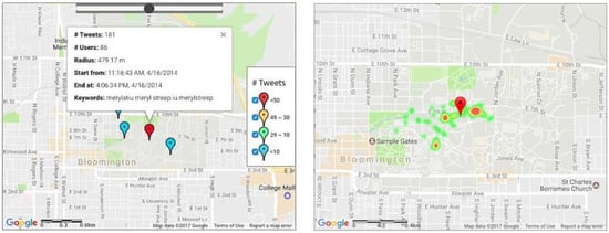
Figure 10.
Clusters of the tweets about Meryl Streep’s visit to Indiana University on 16 April 2014 and the tweets distribution of the most significant cluster.
For the temporal pattern in Figure 11a, the start time was between 1:00 PM and 1:30 PM. Before the event began, there were some scatter tweets; and after 3:30 PM, this activity faded out, which hinted that the lecture was over. These patterns were not only shown via the Twitter data but were also consistent with the local news article. From the word frequency in Figure 11b, the hottest words were related to the name “Meryl Streep.” Other hot words like “honorary” and “university” reflected that the event was relevant to the honorary degree that Meryl Streep received.
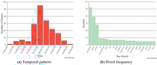
Figure 11.
Temporal pattern and word frequency of Meryl Streep’s visit to Indiana University on 16 April 2014: (a) Temporal pattern; and (b) Word frequency.
For the topics modeled in Table 5, Topics 2 and 4 were about normal school activities and they did not mention Meryl Streep. Topics 1, 3, 5 and 6 all discussed Meryl Streep to some degree. Among all these topics, Topic 5 was the most significant topic and was all about Meryl Streep and the event and also disclosed the location of the event.
Table 5.
Modeled topics of Meryl Streep’s visit to Indiana University.
4.3. Detection of Recurring Events
When studying the events in Ann Arbor MI, two clusters occurred in October 2015 that caught our attention. As shown in Figure 12, the centers of both clusters were in the University of Michigan Football Stadium and they were close to each other. Moreover, other features were similar, such as the number of tweets, the number of users, temporal patterns and even the word frequency patterns. For the cluster on 10 October, there were 228 tweets generated by 183 users. For another cluster on 17 October, there were 237 tweets generated by 199 users. The most frequently used words of both clusters were the same: “Michigan,” “big,” “stadium,” “house,” and “blue.” According to the location of the clusters and the keyword “football” in both word frequency charts, we concluded that University of Michigan football games were held on 10 and 17 October.
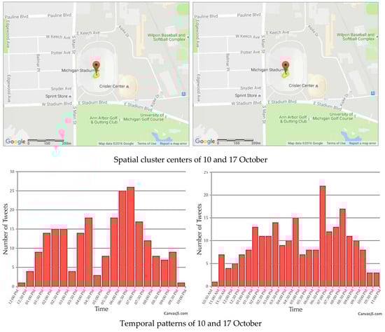
Figure 12.
Spatial patterns (top) and temporal patterns (bottom) of tweets during the football games at Michigan Stadium on 10 October (left) and 17 October (right) of 2015.
As shown in Table 6, many keywords overlapped in the frequency charts for these two games. In both keyword lists, “blue,” “goblue” and “wolverines” caught our attention, as the school color of the University of Michigan is blue and the nickname of the football team is the Wolverines. In the chart for 10 October, the keywords “northwestern” and “wildcats” referred to the team of Northwestern University, while in the chart for 17 October “msu” and “Spartans” referred to the football team of Michigan State University. Thus, we reasonably concluded that the Wolverines’ opponents in these two games were the Wildcats and the Spartans. Besides the basic information about the games, the most important thing that we wanted to know was the performance of the teams. Although “blue” and “goblue” in both games were similar, their frequency on 17 October was less than on 10 October. It seems that the fans of the University of Michigan were less enthusiastic in their support for their team in regard to tweeting for the second game on 17 October. Another clue is that “gogreen” appeared in the word frequency chart of the second game, which is opposite of “goblue.” With all these clues, we could tell that, in the second game, the Wolverines received less support and more resistance than in the first game.
Table 6.
Word frequency of the football games at the Michigan Stadium on 10 Oct. (*/) & 17 (/*), 2015.
As for the topics, there were also some differences in the similarities of the word frequency charts. Table 7 shows the four topics from both games. For Topics 1 and 3, although there were differences as far as the importance of some words, both games performed similarly on the top word and were mostly related to the home team. In Topic 2, the visiting teams were different, which affected the words used. The biggest differences were in Topic 4. The topic on 10 October was more related to the home team, such as “michigan” and “goblue,” while the topic on 17 October demonstrated a different pattern and no top words were highly related to the home team but were rather words such as “msu” and “gogreen,” which represented the visiting team. In summary, the performance of the Wolverines in the game on 17 October was not as good as the one on 10 October.
Table 7.
Modeled topics for the football games at University of Michigan on 10 and 17 October 2015.
According to the game records in FBschedules.com [53], there were, in fact, two football games on these two dates. On 10 October 2015, the opponent was the Northwestern Wildcats and the Michigan Wolverines won handily 38–0, which explained the “380” in Topic 4. On 17 October 2015, the opponent was the Michigan State Spartans, which the Michigan Wolverines lost 27–23. These news reports supported our analysis. It should be noted that beside the recurring events such as the two football games in Ann Arbor in October 2015, we also found that the Bloomington Craft Beer Festival not only happened in April 2014 but happened at the same location in April 2015.
5. Discussion
5.1. Parameter Selections
Obtaining reliable clustering results is key to successful event detection, which can be achieved by carefully selecting several parameters in the method. For spatial-temporal clustering, ST-DBSCAN requires four input parameters: (1) maximum spatial distance value (d1), (2) maximum temporal distance value (d2), (3) minimum number of points within d1 and d2 distance (minPts) and (4) threshold for inclusion in a cluster (δd). According to Ester et al. (1996), there is a simple heuristic way to estimate the number of d1 and minPts, which suggests minPts = ln(n), where n is the size of the data. It then applies k nearest neighbors for each point, where k is equal to minPts. Next, we could plot a sorted graph for the values of k- distance. The first “valley” of the graph is the d1 that we need. Theoretically, this method could provide good estimates for minPts and d1. However, the estimation of parameters depends upon the size of the data set (n) and spatial distribution patterns, while the inner characteristics of events may not highly correlate to the full data set.
To address this problem, with the knowledge we gained on event detection, some of the tested values were found to make this task easier. For d1, 100 m could cover most events while reducing noise. For d2, 30 min appeared to be a good fit. Although some events could last for several hours, most of them cannot maintain that many points in every 30-min period. For minPts, 10 was a reasonable number to avoid non-significant, random chats among tweet users. For δd, its functionality is to set up a boundary clarification of two clusters. Because we do not have prior knowledge of the duration of events, this parameter was ignored in our experiments.
After the emergence of ST-DBSCAN, several clusters were produced and two new parameters were introduced: minimum number of involved users (minUsers) and minimum frequency of the top word (minFw). These two parameters further filtered clusters after ST-DBSCAN clustering. For minUsers, if a cluster had only a few users involved, the event correlated to this cluster was unlikely to have much social impact and was likely to be an event that only a few people were talking in turns. Providing a threshold for the number of users can reduce that noise. For minFw, if the frequency of the hottest word was small, all other words were of low frequency. In this case, the topics were highly diversified and this cluster was likely to be random. Figure 13 shows good noise filtering after applying the constraints of minUsers and minFw. The examples in this paper all had the following set of parameters: 100 m for d1, 30 min for d2, 10 for minPts, 2 for minUsers and 5 for minFw.
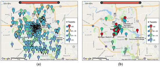
Figure 13.
Effects of ST-DBSCAN parameters on clustering results in February 2014 in Ann Arbor: (a) without constraints of minUsers and minFw; and (b) with minUsers as 2 and minFw as 5.
A sensitive parameter for LDA is the number of potential topics (K). According to Blei et al. [39], perplexity, that is, the level of mixture or confusion, is recommended as a criterion for performance evaluation: the lower the perplexity, the better the model [54]. A practical method of perplexity estimation is to plot the relation graph between K and perplexity and then choose the K with the perplexity. But according to Chang et al. [55], the predictive likelihood (or equivalently, perplexity) for topic modeling and human judgment on topics are often not correlated and sometimes may even be slightly anti-correlated instead. In this case, we still applied the best guess of K based on the plot between K and perplexity but made an adjustment to it according to the topic structure of the sentences and the number of sentences attached to specific topics. Table 8 shows an example of the relation between the perplexity and the number of topics, ranging from 2 to 10. In this case, six would be the proper number of topics because of the lowest perplexity.
Table 8.
Perplexity vs #topics of the major cluster for the gunshot in West Lafayette, IN.
The use of hashtags may cause difficulties in text mining, however, it is very convenient for Twitter users. For example, “#prayforpurdue” and “#bloomingtoncraftbeerfest” represent “pray for Purdue” and “Bloomington Craft Beer Fest,” respectively. However, our workflow considered a hashtag as an individual word instead of a combination of several words. Another example of limitation is word abbreviation. For example, “cod” is short for “Call of Duty,” a PC game, in a cluster but it may have other meanings in other contexts, which requires extra effort to understand the meaning of the words and resolve such ambiguities.
5.2. Event Details Revealed and Understood
Successful event detection can reveal properties and details about the events. The gunshot in West Lafayette IN and the St. Patrick’s Day celebration in Columbus OH were two examples of our retrieval of known events. For the gunshot in West Lafayette IN, we determined that the outbreak of tweets occurred around 12:15 PM and we identified the locations where many users were talking about this incident. We also identified several central topics about this news, such as general information related to the gunshot, the location of the gunshot, the reaction of the students and the police and the feelings of the students after the gunshot. For the St. Patrick’s Day celebration in Columbus OH, we found that the most popular locations of the tweets were around the campus of The Ohio State University. Our research revealed some of the impact of this event among the users. This event also introduced a name problem, that is, when people used different words to refer to “Patrick,” such as “Pat,” “Patty,” and “Paddy.” The fact that different words might indicate the same meaning could diffuse the actual impact of the central words as a result of the transformations.
The Beer Festival in Bloomington and the football games in Ann Arbor are two examples of our success in discovering events. The beer festival in Bloomington was concentrated in a particular location so its temporal pattern also matched the event information. For the textual information, since most Twitter users were using similar sentence structures when tweeting, it was easy to identify the event based on the word frequency. For the football games in Ann Arbor, we discovered that there were two games within one week. These two games had similar spatial and temporal patterns but different textual information patterns. The game on 10 October 2015 was dominated by the Wolverines of the University of Michigan, while the other game on 17 October 2015 did not show as many home advantage tweets and the University of Michigan lost that game. This difference helped us determine the performance of the teams, which was supported by the news reports.
The gunshot in West Lafayette IN and the St. Patrick’s Day celebration in Columbus OH are well-known events in those two cities. The patterns of these events revealed their features and influence on the general public. In the case of the gunshot in West Lafayette, we compared the effects of applying different settings of the parameters, showing that larger thresholds for parameters were preferred when dealing with an event. For St. Patrick’s Day in Columbus, we revealed that one central meaning can be represented by many words, which could affect the accuracy of the results.
Our unknown events, the beer festival and Meryl Streep’s visit, both were concentrated around a particular central area and there were significant features that allowed us to form conclusions regarding the basic details of the events through our results. In the case of the beer festival, we determined that if the tweets followed the same pattern, it would be much easier to extract the textual information and its internal relations. For Meryl Streep’s visit, the spatial and temporal patterns were consistent with the news reports but because many topics were discussed in her lecture, it was not easy to summarize the full lecture.
For recurring events, either known or unknown, the tweets about the two football games in Ann Arbor followed similar patterns. The textual information told us that the events were football games and revealed the game results to a certain degree.
6. Conclusions
Our study explored the use of Twitter data to detect real-world events. We found that to make this possible and reliable, different methods were needed to target events at varying scales. For small- scale community level events, a sequential clustering strategy, starting with spatial-temporal clustering, followed by sematic clustering, is a reasonable choice, especially when the intent is to detect latent or unknown events.
Based on this understanding and perspective, we introduced a workflow into our study to reveal spatial and temporal patterns and to understand the semantics of the events, which we verified using three types of events: known events, unknown events and recurring (either known or unknown) events. We successfully utilized Twitter data for the four cities where the events of interest occurred and determined that ST-DBSCAN provided satisfactory, reliable results. Metadata of the clusters were able to filter themselves, from which only the clusters with focused, meaningful textual information were selected. LDA was used to classify the tweets in a spatial-temporal cluster into several reasonable topics, which helped us understand the structure of the textual information and the semantic nature of the event.
All these examples demonstrated that Twitter could be utilized to discover real-world events as well as to understand their intrinsic behaviors. However, there were some limitations in the research. The use of Twitter data may result in biases in a social study [10,56,57]. For spatial and temporal studies like ours, Twitter users need to enable the geo-tag function. The motivation of users to do this are unknown, which means that the dataset we collected may not be randomly sampled among all Twitter users. Also, because the number of geo-tagged tweets represented only ~2% of the total tweets, most events that happen in the real world are not recorded by geo-tagged tweets. In this case, the Twitter data are able to reveal only some events. Not every event in the real world may find a match in the Twitter data. Nevertheless, exploring Twitter data is still an efficient means for geosocial science studies because of its extremely large user population.
Other limitations stem from the workflow and methodology. We found that the processing of textual information does not include UTF-8 characters, such as emojis, or languages other than English. Moreover, for events that last for several days, such as a graduation commencement, extra effort is required for combining data. There are also some limitations in textual information processing, for example, hashtag parsing.
One possible future direction of our research concerns the techniques used, with the objective of providing meticulous parameters for ST-DBSCAN when revealing different types of events or proposing a better algorithm for filtering the spatio-temporal information. Also, having a better understanding of textual information can facilitate the interpretation of the events. We used only the basic LDA algorithm in topic clustering but some advanced algorithms may be able to better depict the textual information. Another future direction of this research is to incorporate various types of datasets, such as data from other social media, point of interest (POI) data, address data, traffic data, census data and economic data. This combined use of heterogeneous data can be expected to carry out a coherent analysis of the nature of an event and its location and time, determine their correlation and ultimately explore and answer the “why” part of an event for geo-social science studies.
Author Contributions
Yue Li and Yuqian Huang collected the data. Yuqian Huang carried out the tests and wrote the early version of the work under the advisory of Jie Shan. All authors wrote the paper and contributed to its revision.
Conflicts of Interest
The authors claimed no conflict of interest.
References
- Milstein, S.; Lorica, B.; Magoulas, R.; Hochmuth, G.; Chowdhury, A.; O’Reilly, T. Twitter and the micro-messaging revolution. In Communication, Connections, and Immediacy–140 Characters at a Time; O’Reilly Media, Inc.: Champaign, IL, USA, 2008. [Google Scholar]
- Kwak, H.; Lee, C.; Park, H.; Moon, S. What is Twitter, a social network or a news media? In Proceedings of the 19th International Conference on World Wide Web, Raleigh, NC, USA, 26–30 April 2010; ACM: New York, NY, USA, 2010; pp. 591–600. [Google Scholar]
- Statista—The Statistics Portal. Number of monthly active international Twitter users from 1st quarter 2010 to 4th quarter 2017 (in millions) 2018. Available online: https://www.statista.com/statistics/274565/monthly-active-international-twitter-users/ (accessed on 12 February 2018).
- Kwan, M.-P. Algorithmic geographies: big data, algorithmic uncertainty, and the production of geographic knowledge. Ann. Assoc. Am. Geogr. 2016, 106, 274–282. [Google Scholar]
- Miller, G. Social scientists wade into the tweet stream. Science 2011, 333, 1814–1815. [Google Scholar] [CrossRef] [PubMed]
- Morales, A.J.; Vavilala, V.; Benito, R.M.; Bar-Yam, Y. Global patterns of synchronization in human communications. J. R. Soc. Interface 2017. [Google Scholar] [CrossRef] [PubMed]
- Leetaru, K.; Wang, S.; Cao, G.; Padmanabhan, A.; Shook, E. Mapping the global Twitter heartbeat: The geography of Twitter. First Monday 2013, 18, 4–5. [Google Scholar] [CrossRef]
- Grandjean, M. A social network analysis of Twitter: Mapping the digital humanities community. Cogent Arts Humanit. 2016, 3, 1171458. [Google Scholar] [CrossRef]
- Hahmann, S.; Purves, R.S.; Burghardt, D. Twitter location (sometimes) matters: Exploring the relationship between georeferenced tweet content and nearby feature classes. J. Spat. Inf. Sci. 2014, 9, 1–36. [Google Scholar] [CrossRef]
- Sloan, L.; Morgan, J. Who tweets with their location? Understanding the relationship between demographic characteristics and the use of geoservices and geotagging on Twitter. PLoS ONE 2015, 10, e0142209. [Google Scholar] [CrossRef] [PubMed]
- Li, Y.; Li, Q.; Shan, J. Discover patterns and mobility of twitter users—A study of four U.S. college cities. ISPRS Int. J. Geo-Inf. 2017, 6, 42. [Google Scholar] [CrossRef]
- Jurgens, D.; McCorriston, J.; Ruths, D. Geolocation prediction in Twitter using social networks: A critical analysis and review of current practice. In Proceedings of the 9th International Conference on Web and Social Media (ICWSM-15), Oxford, UK, 26–29 May 2015. [Google Scholar]
- Patel, N.; Stevens, F.R.; Huang, Z.J.; Gaughan, A.E.; Elyazar, I.; Tatem, A.J. Improving large area population mapping using geotweet densities. Trans. GIS 2017, 21, 317–331. [Google Scholar] [CrossRef] [PubMed]
- Montasser, O.; Kifer, D.V. Predicting demographics of high-resolution geographies with geotagged tweets. In Proceedings of the Thirty-First AAAI Conference on Artificial Intelligence (AAAI-17), San Francisco, CA, USA, 4–10 February 2017. [Google Scholar]
- De Bruijn, J.A.; de Moel, H.; Jongman, B.; Wagemaker, J.; Aerts, J.C.J.H. TAGGS: Grouping tweets to improve global geoparsing for disaster response. J. Geovisualization Spat. Anal. 2018, 2, 2. [Google Scholar] [CrossRef]
- Nguyen, O.C.; McCullough, M.; Meng, H.-W.; Paul, D.; Li, D.P.; Kath, S.; Loomis, G.; Nsoesie, E.O.; Wen, M.; Smith, K.R.; et al. Geotagged U.S. tweets as predictors of county-level health outcomes, 2015–2016. Am. J. Public Health 2017, 107, 1776–1782. [Google Scholar] [CrossRef] [PubMed]
- Chaniotakis, E.; Antoniou, C.; Aifadopoulou, G.; Dimitriou, L. Inferring activities from social media data. Transp. Res. Record: J. Transp. Res. Board 2017, 2666, 29–37. [Google Scholar] [CrossRef]
- Hong, I.; Jung, J.-K. What is so “hot” in heatmap? Qualitative code cluster analysis with foursquare venue. Cartographica 2017, 52, 332–348. [Google Scholar] [CrossRef]
- Yang, Y.; Pierce, T.; Carbonell, J. A study of retrospective and on-line event detection. In Proceedings of the 21st Annual International ACM SIGIR Conference on Research and Development in Information Retrieval, Melbourne, Australia, 24–28 August 1998; ACM: New York, NY, USA, 1998; pp. 28–36. [Google Scholar]
- Crampton, J.W.; Graham, M.; Poorthuis, A.; Shelton, T.; Stephens, M.; Wilson, M.W.; Zook, M. Beyond the geotag: situating ‘big data’ and leveraging the potential of the geoweb. Cartogr. Geogr. Inf. Sci. 2013, 40, 130–139. [Google Scholar] [CrossRef]
- Phuvipadawat, S.; Murata, T. Breaking news detection and tracking in Twitter. In Proceedings of the 2010 IEEE/WIC/ACM International Conference on Web Intelligence and Intelligent Agent Technology (WI-IAT), Toronto, ON, Canada, 31 August–3 September 2010; Volume 3, pp. 120–123. [Google Scholar]
- Lee, R.; Sumiya, K. Measuring geographical regularities of crowd behaviors for Twitter-based geo-social event detection. In Proceedings of the 2nd ACM SIGSPATIAL International Workshop on Location-based Social Networks, San Jose, CA, USA, 3–5 November 2010; ACM: New York, NY, USA, 2010; pp. 1–10. [Google Scholar]
- Weng, J.; Lee, B.-S. Event detection in Twitter. ICWSM 2011, 11, 401–408. [Google Scholar]
- Pennacchiotti, M.; Popescu, A.-M. A machine learning approach to Twitter user classification. ICWSM 2011, 11, 281–288. [Google Scholar]
- Benson, E.; Haghighi, A.; Barzilay, R. Event discovery in social media feeds. In Proceedings of the 49th Annual Meeting of the Association for Computational Linguistics: Human Language Technologies-Volume 1, Portland, OR, USA, 19–24 June 2011; Association for Computational Linguistics: Stroudsburg, PA, USA, 2011; pp. 389–398. [Google Scholar]
- Sakaki, T.; Okazaki, M.; Matsuo, Y. Earthquake shakes Twitter users: Real-time event detection by social sensors. In Proceedings of the 19th International Conference on the World Wide Web, Raleigh, NC, USA, 26–30 April 2010; ACM: New York, NY, USA, 2010; pp. 851–860. [Google Scholar]
- Sakaki, T.; Okazaki, M.; Matsuo, Y. Tweet analysis for real- time event detection and earthquake reporting system development. IEEE Trans. Knowl. Data Eng. 2013, 25, 919–931. [Google Scholar] [CrossRef]
- Walther, M.; Kaisser, M. Geo-spatial event detection in the twitter stream. In Proceedings of the European Conference on Information Retrieval, Moscow, Russia, 24–27 March 2013; Springer: Berlin/Heidelberg, Germany, 2013; pp. 356–367. [Google Scholar]
- Huang, Q.; Wong, W. Modeling and visualizing regular human mobility patterns with uncertainty: An example using Twitter data. Ann. Assoc. Am. Geogr. 2015, 105, 1179–1197. [Google Scholar] [CrossRef]
- MacQueen, J. Some methods for classification and analysis of multivariate observations. In Proceedings of the Fifth Berkeley Symposium on Mathematical Statistics and Probability; University of California Press: Oakland, CA, USA, 1967; Volume 1, pp. 281–297. [Google Scholar]
- Dempster, A.P.; Laird, N.M.; Rubin, D.B. Maximum likelihood from incomplete data via the EM algorithm. J. R. Stat. Soc. Ser. B (Methodol.) 1977, 39, 1–38. [Google Scholar]
- Sander, J.; Ester, M.; Kriegel, H.-P.; Xu, X.-W. Density-based clustering in spatial databases: The algorithm DBSCAN and its applications. Data Mining Knowl. Discov. 1998, 2, 169–194. [Google Scholar] [CrossRef]
- Ankerst, M.; Breunig, M.; Kriegel, H.-P.; Sander, J. OPTICS: Ordering points to identify the clustering structure. In ACM Sigmod Record; ACM: New York, NY, USA, 1999; Volume 28, pp. 49–60. [Google Scholar]
- Kailing, K.; Kriegel, H.-P.; Kröger, P. Density-connected subspace clustering for high-dimensional data. In Proceedings of the 2004 SIAM International Conference on Data Mining (SDM04), Philadelphia, PA, USA, 22 March 2004; SIAM: Philadelpha, PA, USA; Volume 4. [Google Scholar]
- Kulldorff, M. A spatial scan statistics. Commun. Stat.-Theory Methods 1997, 26, 1481–1496. [Google Scholar] [CrossRef]
- Wikipedia. Topic Model. 27 September 2016. Available online: https://en.wikipedia.org/wiki/Topic_model (accessed on 18 October 2016).
- Deerwester, S.; Dumais, S.T.; Furnas, G.W.; Landauer, T.K.; Harshman, R. Indexing by latent semantic analysis. J. Am. Soc. Inf. Sci. 1990, 41, 391. [Google Scholar] [CrossRef]
- Hofmann, T. Probabilistic latent semantic indexing. In Proceedings of the 22nd Annual International ACM SIGIR Conference on Research and Development in Information Retrieval, Berkeley, CA, USA, 15–19 August 1999; ACM: New York, NY, USA, 1999; pp. 50–57. [Google Scholar]
- Blei, D.M.; Ng, A.Y.; Jordan, M.I. Latent Dirichlet allocation. J. Mach. Learn. Res. 2003, 3, 993–1022. [Google Scholar]
- Beli, D.M.; Griffiths, T.L.; Jordan, M.I.; Tenenbaum, J.B. Hierarchical topic models and the nested Chinese restaurant process. In Advances in Neural Information Processing Systems; MIP Press: Cambridge, MA, USA, 2004; pp. 17–24. [Google Scholar]
- Teh, Y.W. A hierarchical Bayesian language model based on Pitman-Yor processes. In Proceedings of the 21st International Conference on Computational Linguistics and the 44th Annual Meeting of the Association for Computational Linguistics, Sydney, Australia, 20 July 2006; Association for Computational Linguistics: Stroudsburg, PA, USA, 2006; pp. 985–992. [Google Scholar]
- Birant, D.; Kut, A. ST-DBSCAN: An algorithm for clustering spatial–temporal data. Data Knowledge Eng. 2007, 60, 208–221. [Google Scholar] [CrossRef]
- Ester, M.; Kriegel, H.-P.; Sander, J.; Xu, X.W. A density-based algorithm for discovering clusters in large spatial databases with noise. In Proceedings of the KDD, Portland, Oregon, USA, 2–4 August 1996; Volume 96, pp. 226–231. [Google Scholar]
- Allahyari, M.; Pouriyeh, S.; Assefi, M.; Safaei, S.; Trippe, E.D.; Gutierrez, J.B.; Kochut, K. A Brief Survey of Text Mining: Classification, Clustering and Extraction Techniques. arXiv, 1707; arXiv:1707.02919v2. [Google Scholar]
- Jelodar, J.; Wang, Y.; Yuan, C.; Feng, X. Latent Dirichlet Allocation (LDA) and Topic modeling: models, applications. A Survey. arXiv, 1711; arXiv:1711.04305v1. [Google Scholar]
- Krestel, R.; Fankhauser, P.; Nejdl, W. Latent Dirichlet allocation for tag recommendation. In Proceedings of the Third ACM Conference on Recommender Systems, New York, NY, USA, 23–25 October 2009; ACM: New York, NY, USA, 2009; pp. 61–68. [Google Scholar]
- Porteous, I.; Newman, D.; Ihler, A.; Asuncion, A.; Smyth, P.; Welling, M. Fast collapsed Gibbs sampling for latent Dirichlet allocation. In Proceedings of the 14th ACM SIGKDD International Conference on Knowledge Discovery and Data Mining, Las Vegas, NV, USA, 24–27 August 2008; ACM: New York, NY, USA, 2008; pp. 569–577. [Google Scholar]
- Twitter. The Streaming APIs Overview. 2014. Available online: https://dev.twitter.com/streaming/overview (accessed on 18 October 2016).
- Purdue University. Victim, Suspect Identified in Purdue Campus Shooting. 2014. Available online: https://www.purdue.edu/newsroom/releases/2014/Q1/purdue-police-confirm-1-fatality,-1-in-custody-following-campus-shooting.html (accessed on 18 October 2016).
- Wikipedia. Saint Patrick’s Day. 11 October 2016. Available online: https://en.wikipedia.org/wiki/Saint_Patrick%27s_Day (accessed on 18 October 2016).
- Bloom Magazine. Bloomington Craft Beer Festival. 2014. Available online: http://www.magbloom.com/events/bloomington-craft-beer-festival/ (accessed on 21 November 2016).
- Indiana University Bloomington. Meryl Streep Will Receive an Honorary Doctoral Degree. 2014. Available online: http://archive.news.indiana.edu/releases/iu/2014/02/meryl-streep-honorary-doctorate.shtml (accessed on 22 February 2017).
- FBschedules.com. 2015 Michigan Wolverines Football Schedule. 2015. Available online: http://www.fbschedules.com/ncaa-15/big-ten/2015-michigan-wolverines-football-schedule.php (accessed on 21 November 2016).
- Wallach, H.M.; Murray, I.; Salakhutdinov, R.; Mimno, D. Evaluation methods for topic models. In Proceedings of the 26th Annual International Conference on Machine Learning, Montreal, QC, Canada, 14–18 June 2009; ACM: New York, NY, USA, 2009; pp. 1105–1112. [Google Scholar]
- Chang, J.; Gerrish, S.; Wang, C.; Boyd-Graber, J.L.; Blei, D.M. Reading tea leaves: How humans interpret topic models. In Advances in Neural Information Processing Systems; MIP Press: Cambridge, MA, USA, 2009; pp. 288–296. [Google Scholar]
- Malik, M.M.; Lamba, H.; Nakos, C.; Pfeffer, J. Population bias in geotagged tweets. In Standards and Practices in Large-Scale Social Media Research: Papers from the 2015 ICWSM Workshop; AAAI Press: Palo Alto, CA, USA, 2015; pp. 18–27. [Google Scholar]
- Tasse, D.; Liu, Z.; Sciuto, A.; Hong, J.I. State of the Geotags: Motivations and Recent Changes. In Proceedings of the Eleventh International AAAI Conference on Web and Social Media (ICWSM 2017), Montreal, QC, Canada, 15–18 May 2017. [Google Scholar]
© 2018 by the authors. Licensee MDPI, Basel, Switzerland. This article is an open access article distributed under the terms and conditions of the Creative Commons Attribution (CC BY) license (http://creativecommons.org/licenses/by/4.0/).