1. Introduction
Coastal erosion has been a worldwide issue since the early 1900s, and the risks and hazards related to its processes are increasing as the number of people living in coastal areas is impressive: about 86 million within 10 km from the coastline in Europe alone in accordance with the reports of European Topic Centre on Climate Change Adaptation (ETC-CCA) [
1]. Coasts and beaches are crucial for the economy of many countries, because access to the sea provides the chance to intensify trading, resource exploitation and tourism, which is the main revenue for many communities. In this sense, protection of the coasts is a priority, because erosion processes are (i) progressively putting municipalities in jeopardy, which need to build expensive defense structures, and (ii) reducing beach width, which hampers profits coming from activities such as tourism.
The consequences of the erosion affect also the environment, because several habitats are endangered by coastal retreat [
2]. For instance, coastal dunes are most affected by sediment loss from the beach, because wave run-up reaches higher distances on the backshore up to the base of the dunes [
3]. This implies huge volume loss and dune retreat or destruction [
4,
5,
6] and consequently severe problems for the vegetation [
7,
8,
9]. In general terms, coastal erosion occurs in sediment-starving settings: the particles naturally feeding a specific sector of coast no longer compensate those that are wiped out by waves and currents. River bedload is the most important source of beach sediments: due to multiple factors (e.g., river damming, bank armoring, sediment quarrying from the river bed), during the last century, river sediment load has decreased exceptionally, which ultimately had led to the first erosion processes.
As the hard structures (groynes, breakwaters) built to protect the coastal areas often turned out to be a failure in the long term (because of side-effects that emphasize localized retreats), recently, coastal managers have preferred to apply softer approaches involving sand redistribution [
10]. Artificial replenishment and sand backpassing/bypassing are increasingly used to restore a suffering beach [
11,
12,
13], because they are intended not to overly modify the previous configuration of the coast. The downside of beach fills is the frequent (seasonal to annual) need to integrate the replenishment as waves and currents keep on moving and redistributing the sand, because they do not act to solve the main problem, which is river sediment load diminution. For all these reasons, increasing the knowledge about sediment transport is crucial to gain more information about particle redistribution along and across the beach. In particular, a better definition of transport pathways on sandy beaches would provide an optimization of the interventions in terms of durability, not to mention the possible savings generated by a more accurate sizing of the replenishment. In addition, it would be of major help for the conservation of dunes, both as geomorphological features and as a species habitat. As a matter of fact, lately, dune restoration has been often utilized as an additional soft approach along with replenishment and sand redistribution [
14,
15].
2. State of the Art
Sand transport has long been studied and analyzed because of the decisive role it has in virtually every depositional environment [
16,
17].
First attempts to measure sediment transport rates were made by means of mechanical devices such as sediment traps, which resulted in being useful because they provided actual measurements of sand moving in given time spans [
18,
19]. Besides, the amount of sediment trapped inside the mechanism would be matched with the flow recorded during that same time frame to give invaluable insights about wind and transported sand [
20]. However, the main issues related to this technique are the need to get to the installation site to empty the basket of the trap (once full it would not work anymore) and the fact that in extended working periods, it is not possible to discriminate the transport rate recorded under a definite flow condition.
Another simple concept that has been applied to sediment transport is tracing particles in order to identify the displacement after specific time spans. This technique is particularly suitable to coarse-clastic beaches, where the coarser grain-size makes it easier to mark single samples. After attempts made by painting gravel particles [
21], using allochthonous lithologies [
22], and coupling pebbles to electronic devices [
23], the technology that produced better results in terms of recovery rate was the Radio Frequency IDentification (RFID). Individual pebbles would be unequivocally identified by a passive transponder activated by the low frequency radio signals transmitted by an antenna [
24,
25]. Though useful for many purposes, this method does not provide any clue about the trajectories the tracers underwent between the recoveries.
Tracing techniques have also been applied to sand beaches, even though the results were not as successful as on coarse-clastic beaches. In particular, sand composition [
26,
27] and bioclasts [
28,
29] have been used as natural tracers; fluorescent [
30,
31] and radioactive [
32] tracers have been used as artificial tracing techniques. Another method to infer sediment transport is frequent topographic surveying [
33,
34]. The most intense modifications to the beach profile are achieved during storms, as high-energy waves deeply rework the subaerial and underwater portions of the beach. Therefore, the comparison between the topographic configuration before and after storms would provide the basis for volume shift calculations. The same end results can be obtained with remote sensing technologies, such as LiDAR [
35,
36] and satellite imagery [
37,
38]. As for sediment tracing, these techniques do not provide sensible information about sand movement during the periods when it should occur the most: the high-energy events. For all these reasons, instruments able to record data series in real time and for prolonged periods, including storms, would provide significant improvements for a better definition of sediment transport.
Wireless Sensor Networks (WSN) represent in many cases a good option for in situ monitoring infrastructures since they allow continuous, remote and real-time data acquisition. WSN-based monitoring infrastructures have been developed for a wide range of scenarios [
39,
40], and several applications can be found for environmental monitoring [
41,
42]. The deployment of WSNs in coastal and marine environments has been widely discussed [
43,
44]: anyway, the greater part of the applications focus on the measurement of water quality [
45] and atmospheric parameters [
46], while to our knowledge, no solution exists focusing on beach morphology as the one proposed in this paper.
A comparative analysis about the state of the art methods and the proposed WSN solution, focusing on both the advantages and drawbacks, is provided in
Table 1.
3. System Architecture
The proposed WSN architecture for the monitoring of sand layer variations is expected to be integrated in a wider IoT framework envisaging the adoption of additional typologies of sensor nodes [
47]: these include weather stations similar to the one presented in [
48], but characterized by lower costs and reduced power consumption (hence lower performances than an ultrasonic station) and able to measure the intensity and direction of wind at three different heights in 2D (excluding the more complex vertical dimension). Another feature of this wider architecture in common with the described applications will be the use of sand traps, to which weight sensors will be added in order to automatically measure the quantity of sand transported by wind and captured by them. The system could also foresee the use of sensors for measuring ground temperature and humidity: these can be important parameters since they strongly affect the transportation of sand (conditions of ground humidity tend to impede sand movement).
Basically, the proposed system relies on existing solutions, enhancing them by adding several technological features and wireless network management and by providing remote, real-time, data control and analysis tools. In this context, particular attention has been devoted to the design and development of the sensor network for the monitoring of height and volume variations of sandy beaches and dunes, and this is the innovative feature of the system herein proposed.
Low cost and reduced energy consumption are the two key requirements of the whole system, thus the choice of tools and instruments for the development of the monitoring devices has fell on the Arduino community, being an open-source project offering small dimension printed circuit boards with a micro-controller and related components, to which several accessories can be connected (e.g., wired and wireless modules, GSM boards for data traffic), providing a wide range of functionalities, in particular for wireless connectivity. The objective was then the realization of a complete system, inexpensive and ready to use, which would allow a user, through an Internet browser, to visualize and manage relevant data in the monitored area.
To achieve this goal, a WSN has been realized: in particular, ad hoc sensors have been designed and developed for measuring the height variations of the sand layer; network organization and communication protocols have been defined; and finally, a data storage and analysis system has been developed through the implementation of a database (MySQL), a web server (Glassfish) and a web application (in Java language).
Specifically, the developed sensor nodes are basically “sensing poles”, whose height is 220 cm and diameter 3 cm, which are expected to be placed in the sand measuring the variation levels through an array of Light-Dependent Resistors (LDRs) (the sensors’ functioning principle will be described in detail in
Section 5.1). The poles are not free to move: actually, they are expected to be stuck into the ground about 100 cm. Thus, in no way could the local dynamics (either wind or wave) offset the sensor nodes. Since the diameter of the poles is very small (3 cm), no significant difference is expected to occur on the two sides: in particular, since the accuracy of the measured value is in the order of 5 cm and a maximum expected difference value of 4 cm is expected, this will not affect the measurements. Recording the exact position of the nodes by a DGPS-RTK (Differential Global Positioning System-Real-Time Kinematic) instrument is crucial since repetitions of data collection campaigns are to be performed periodically in order to compare the results coming from the very same spots. The sensor nodes are expected to be deployed on the backshore of the beach at a level tide fluxes would not reach; the runup of storm waves might reach the sensors, but they would only determine sediment volume displacements, which is what the sensors actually measure. As the system is not invasive, the main factors driving the morphodynamic evolution of a beach, such as wind and waves, are not affected by the sensors. As mentioned, the poles are so thin that sand accumulation because of their presence is negligible, waves reach the sensors for a few seconds only during major storms.
The steps for the realization of the entire system can be summarized as follows:
Design and development of an inexpensive low power ad hoc sensor for monitoring the height variations of the sand layer;
Research and study of the possible techniques for the implementation and configuration of the monitoring network, formed by a network coordinator and several sensor nodes;
Implementation of techniques for the transmission (through ZigBee technology and XBee modules) of data measured by sensors to a coordinator located on the beach and use of GPRS network for real-time data delivery to a web server (data collection center), easily accessible by end users;
Realization of a web application in Java that allows one to receive and store acquired data in a database, for the purpose of allowing the user to monitor network status any time, anywhere.
4. Data Analysis
The data to be collected by the proposed monitoring infrastructure can be used to retrieve different kinds of information according to the number of available sensor nodes and to the different layouts according to which they can be deployed. In any case, in order to process the data with a Geographic Information System (GIS), each deployed node needs to be georeferenced with a high precision Global Navigation Satellite System (GNSS), also measuring the exact elevation of the point: this value is crucial for every kind of data analysis to be carried out. For this purpose, when each sensor node is positioned on the beach or dune, its position is recorded by a DGPS-RTK instrument, which provides accurate values of the coordinates and elevation of the ground at the beginning of data collection.
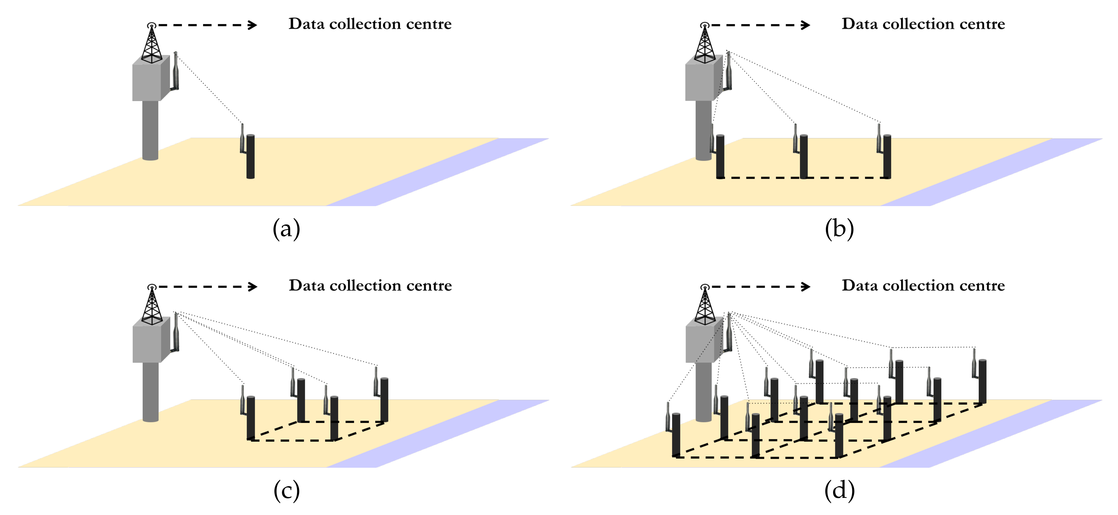
According to the number of available sensor nodes, the following analyses can be carried out:
One node: simple level variation in a specific point of the beach or dune (
Figure 1a).
Two to three nodes: modification of a specific cross-section of the beach or dune (
Figure 1b). This kind of analysis can be crucial if carried out at specific points as, for example, the depression between two adjoining dunes, which are usually the most sensible spots for the erosive processes.
Four nodes: this quantity is the minimum one to allow an assessment of the volumetric variations of an area of limited size (
Figure 1c).
Larger quantities of nodes: arranging them according to a grid layout makes it possible to accurately evaluate the morphological modifications of a relatively large portion of beach or dune, as well as to measure the volumetric variations (
Figure 1d).
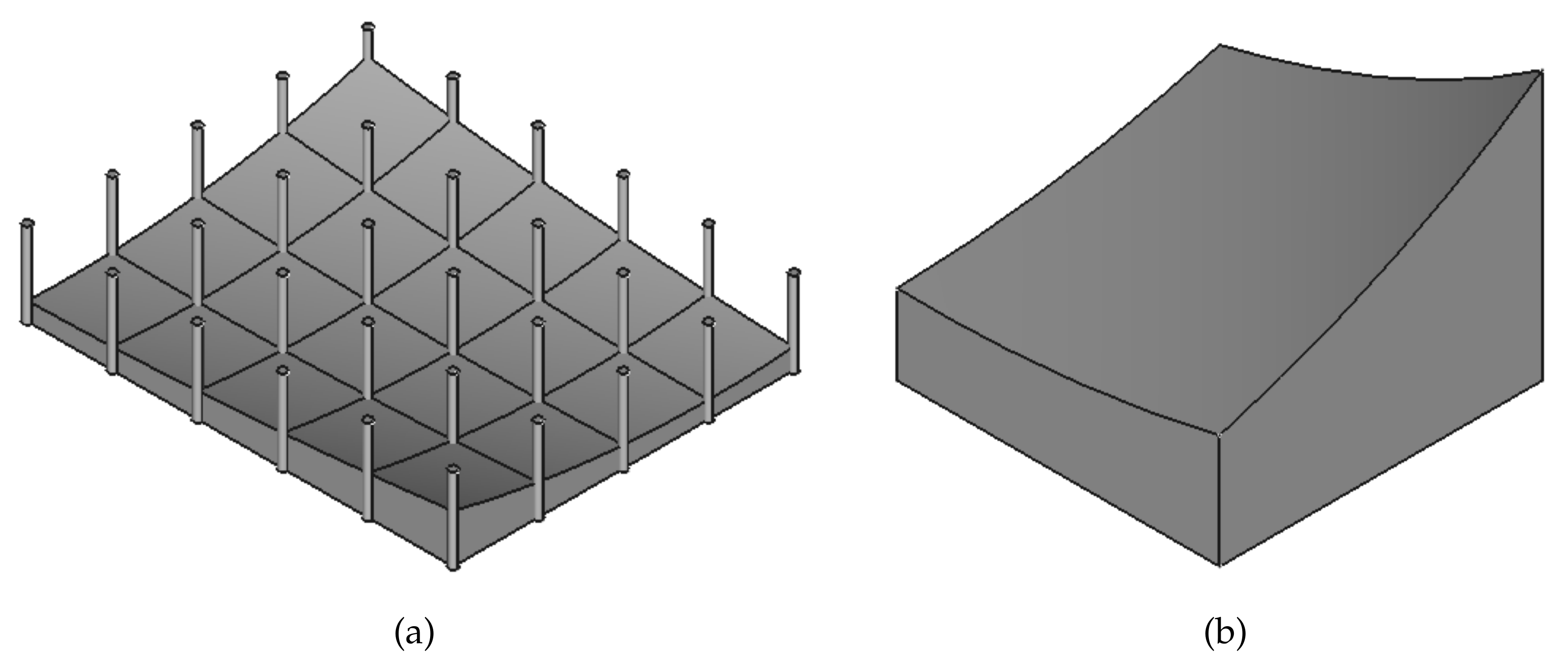
While the first two analyses are simply carried out by comparing the different sand level values and possibly by structuring the data in a GIS, the second two allow the measurement of a wider range of data. In particular, variations of the volume, as well as of the mass of sand can be calculated. Cases 3 and 4 can be considered together since the architecture described in Point 4 is just an extension of the one proposed in Point 3. Combining the measures of the sand level acquired through the sensor network with the exact GNSS position and elevation of the nodes, it is possible to create dynamic 3D maps of the area under study in real time. Indeed,
Figure 2a shows that a portion of beach or dune covered by a large number of sensor nodes can be considered as composed by an array of solids (
Figure 2b), enclosed by four sensor nodes placed at their vertices, that are characterized by a square or rectangular lower base, four trapezoidal side faces that are perpendicular to the base and an irregular upper surface: this one could be flat (when the four upper vertices lie in the same plan), but also curved, concave or convex. The lower base of this solid coincides with the surface of the beach at the deployment instant of the network, while the upper surface is the one delimited by the new sand layer levels measured by the sensor nodes after a predefined span of time.
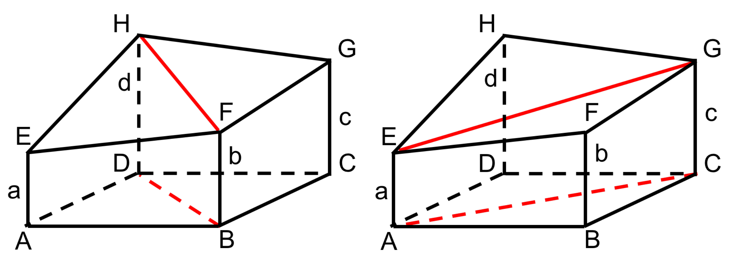
Since the exact calculation of this volume is impossible because the exact shape of the upper surface is not known, an approximation is required. Two ways can be followed: an analytic way based on the interpolation of the four points and then on the volume calculation, or a geometric way based on the approximation of the volume with solid figures and then the use of geometric formulas. The first option would require hard calculations that cannot be carried out by resource-constrained devices such as microcontrollers, forcing then the volume estimation to be moved to the server side of the system, rather than being performed directly on the network coordinator. Moreover, the interpolation carried out on the four points placed at the vertex of a quasi-rectangular surface is expected to lead to an approximation of the surface in the best case only slightly better than the one achievable through the geometric method (but possibly also worse). For this reason, a geometric approach has been chosen, based on the split of the solid into two: in particular, connecting two opposite vertices of the upper base, this one is divided into two surfaces that can be approximated to two triangles. Two subdivisions are possible according to the pair of vertices that is chosen as shown in
Figure 3: a convex one and a concave one. In both cases, the solid is approximately subdivided into two pentahedra with two non-parallel triangular bases and three trapezoidal side faces perpendicular to the lower base. The volume of this figure can be easily calculated through the following formula:
where
A is the area of the lower base, which can be easily calculated since it is a right triangle, and
a,
b and
c are the lengths of the side edges (
Figure 3).
The volumes of the two pentahedra can be summed to obtain an approximated value for the volume of the whole solid enclosed by the four sensor nodes. Since two possible subdivisions of the solid are possible, two different approximate values can be calculated: a larger one for the convex subdivision and a smaller one for the concave. The best approximation for the volume can then be obtained by calculating the two volumes and averaging the two values:
The obtained value is obviously an approximation since it does not take into account small-scale morphological variations. Nevertheless, it is useful to broadly assess the variations in the mass of sand using its density value.
5. The Sensor Node
5.1. Sensor Node Architecture
The idea at the base of the proposed monitoring architecture comes from the need for a tool capable of measuring the temporal variations of sandy beach and dune height variations at different points, in order to assess their progressive morphological modifications, possibly evaluating also the sand volume variations. The developed tool is expected to remain installed on site for a prolonged time; it should be characterized by a certain stability; and it should resist atmospheric conditions that are typical of a harsh environment such as the marine one. According to these requirements, a sensor has been designed for measuring sand level variations with a 5-cm resolution (i.e., a tolerance that has been identified to be adequate for such scenarios according to geologists’ opinion).
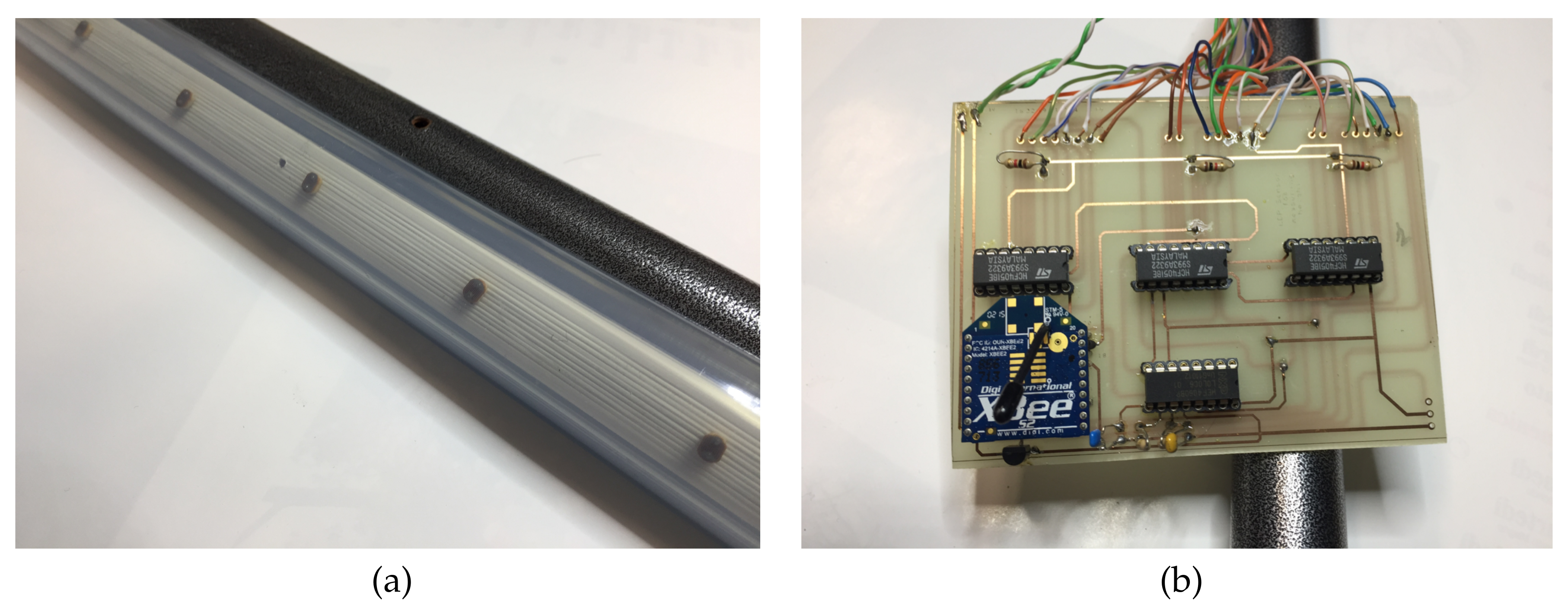
Therefore, a “sensing pole” has been designed and assembled, formed by an array of 24 photo-sensitive resistors (LDR (Light-Dependent Resistors)), positioned at a distance of 5 cm from each other, which convert the intensity of light into a corresponding electric signal. More specifically, a photo-resistor [
49] is an electronic component, the resistance of which is inversely proportional to the intensity of light; thus, it decreases as the light striking the unit increases. This means that the electric current flowing through the resistor is directly proportional to the intensity of light. In such a scenario, a simple sensor (formed by an array of 24 LDRs), opportunely installed, allows one to measure the height variation of a single dune in an easy way: presuming that the pole is inserted in the sand for half of its height and the other half is emerging from the sand, the 12 LDR resistors outside the dunes, being struck by the light, would provide a high output value, while the remaining 12 photo-resistors, covered by the sand, would provide a low value. In this way, by simply counting the number of LDRs characterized by low values, the height of the sand layer can be evaluated (in the proposed system, with 24 LDRs positioned at a 5-cm distance from each other, it would be 60 cm).
Regarding the housing of the sensors, in the marine environment, the hot summer temperatures and the presence of corrosive elements like sand and sea water can easily deteriorate the devices. Hence, the pole has been inserted inside a rubber pipe that is 0.5 cm thick, in order to be protected and insulated: the pipe is totally sealed, and no sand can filter inside; thus, the LDRs are totally protected. Even if a thin layer of sand could stick to the pole, this will not affect the correctness of the measurement since the LDRs proved to be able to detect the presence of sunlight even when covered by a small amount of sand. Obviously, also the related circuit part has been opportunely secured through IP67 protection boxes, appropriate for such scopes.
According to the previous considerations, the main objective of the design was to keep low production costs and to create a sensor with very low energy consumption, which could be powered with simple AA batteries. Then, the overall list of components responding to all the previous requirements is the following:
a wiring mini-channel of 15 × 15 mm dimensions and 2 m height (height of the sensor pole);
a rubber pipe that is 0.5 cm thick, with a diameter of 3 cm and a length of 2 m;
24 VT900 photo-resistors (LDR);
a 14-stage HEF4060BP binary counter, with 10 output buffers;
3 eight-channel HCF4051BE analog Multiplexers (MUX);
a MOSFET transistor, to be used as a switch (BS170);
an IP67 protection box for securing the circuit;
an XBee Series 2 transmission module (for wireless data transmission).
The only components whose cost is significant are the XBee module (around 30$) and the rubber pipe (around 10$), while the sum of the price of all the other components is lower than 20$: this means that the overall node can be built with less than 60$. While this is only a prototype, the price could be notably lowered with an engineered solution to be produced in large quantities.
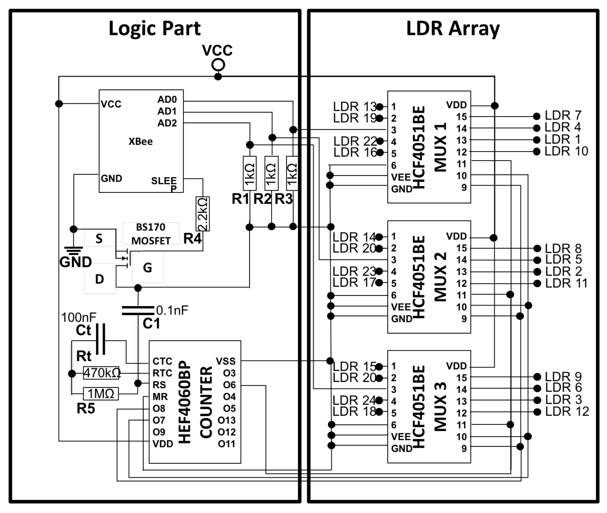
The sensor is composed of three main parts: one part, represented by the pole and the array of sensors (formed by Elements 1–3), carrying out the physical measurement, a logic part, which is formed by Elements 4–7, and the data transmission part, composed of the XBee radio module.
The pole with the sensor array has been realized with a wired mini-channel, on which small holes at a 5-cm distance from each other have been made in order to insert the 24 photo-resistors, for a length of 120 cm (the total length of the pole is 2 m). The electric connection of each single LDR is made in the following way: one of its two terminals is connected to a common power 3-V supply (two AA 1.5-V batteries connected in series), while the other one is connected to one of the eight channels of each of three MUXs (three eight-channel analog multiplexers have been employed, so as to have 3 × 8 = 24 single channels, one for each LDR).
The logic part represents the heart of sensor node, completely defining its operation modality. It allows the sequential selection of the LDRs, allowing the data acquisition from 24 different data sources using only three input lines. Moreover, it manages the duty cycling of the sensor node, allowing power consumption regulation. Finally, an XBee Series 2 radio transmission module allows the data transfer to a gateway in charge of forwarding it to a remote data acquisition center through an Internet connection (see
Section 6).
The circuit diagram of the overall sensor node can be seen in
Figure 4.
5.2. Operating Principle
The data acquisition circuit is powered by two 1.5-V AA batteries in series, providing a total 3 V of voltage. At the circuit activation, the HEF4060BP counter is started. The oscillation frequency being equal to
(with design specifications
K
and
nF), it is easy to calculate the oscillation frequency, which determines the time employed by the counter to change bit status (high-low):
On each pin of the counter (referred to as output buffers Q3–Q9 and Q11–Q13), we have a clock cycle that doubles at each following output. For example, if Q3 needs 2 s to complete a cycle, Q4 and Q5 will employ respectively 4 and 8 s, and so on. The counter outputs control the logical signals for the selection of the MUX: at each change of bit status, the signals select a MUX input to which each single LDR is connected; light intensity perceived by that resistor is measured and acquired through a suitable analog pin of the XBee transmission module. This module delivers the measured value to the network coordinator in wireless mode through the ZigBee protocol. At each transmission, data related to three resistors are delivered (since XBee radio modules are provided with three analog inputs); therefore, for the entire acquisition of the sensed data, eight transmissions are needed. Moreover, there are three logical signals for the selection of the MUX; hence, only three out of 10 possible counter outputs are utilized.
By analyzing and calculating clock cycles at the counter output buffers, it has been considered worthwhile to connect outputs Q6, Q7 and Q8 (i.e., Counter Pins 6, 14 and 13) to the logical selection signals of the three MUX (A, B and C) in the following way:
Counter output Q6 (Pin 6) to logical selection Signal A (Pin 11): Q6 is the output that changes state more frequently, and hence, it is connected to A, which represents the least significant selection bit;
Output Q7 (Pin 14) to logical selection Signal B (Pin 10);
Output Q8 (Pin 13) to logical selection Signal C (Pin 9). C represents the most significant selection bit.
The clock cycle of Q6 output is:
The clock cycle of Q7 output is the double of Q6:
6. Communication Infrastructure
The communication infrastructure is based on a ZigBee network where all the sensor nodes act as ZigBee routers, in order to fully exploit the advantages in terms of reliability and efficiency coming from the implementation of a multi-hop mesh topology: these features allow the network to be resilient with respect to malfunctions of single nodes and to extend the connection coverage to wider areas than the ones achievable with a single-hop IEEE 802.15.4 network.
The smartest device, essential for communication among the different nodes of a WSN, is the ZigBee network coordinator. The coordinator manages network creation and coordination by selecting a suitable radio channel and defining operating parameters (e.g., Personal Area Network (PAN) ID, a 16-bit number for network identification). Once the network is started, it takes the responsibility of maintaining and controlling it and of receiving and processing data coming from all nodes. The hardware part constituting the network coordinator is formed by:
a programmable Arduino UNO electronic board, which determines the operation of the entire network;
an XBee Series 2 transmission module with a related shield to connect it to the Arduino UNO, for wireless (ZigBee) communication between network nodes and the coordinator;
a GSM shield, for the data transmission through GPRS technology from the coordinator to the web server, which makes them accessible in real time.
Small cables have been added to connect the GSM shield to the Arduino through an ICSP (In-Circuit Serial Programming) connector. While this device is characterized by higher production costs than the sensor nodes (around 100$), this does not affect the overall cost of the system since only one coordinator is required for each network.
The main objective being the realization of a low-cost and low-energy WSN, we can envisage simple sensor nodes not equipped with a micro-controller: data are sent to the coordinator as soon as they are acquired, without any processing. Consequently, complexity is shifted to the coordinator side, which should be able to process multiple data. The Arduino board implementing the coordinator has some hardware limitations, among which is a maximum receiving buffer size of 64 byte; therefore, if data are received from multiple sensors, some of them could be discarded due to buffer overflow and then become lost. For each single transmission, a sensor node delivers to the coordinator a 26-byte frame (raw data, not pre-processed); hence, it is not possible to handle more than two nodes at a time if they are transmitting simultaneously.
From multiple tests carried out with the network coordinator receiving and processing data coming from the sensor nodes, it results that the coordinator takes about 7 s to receive, process and transmit a single data-set composed of the readings of three LDRs (this is due to hardware restrictions and the limited processing power of the Arduino UNO used for the implementation of the coordinator, as well as due to the numerous data to be considered). Consequently, the coordinator employs slightly less than one minute (7 s · 8 = 56 s) to acquire, process and transmit all the data coming from a single sensor node. This delay does not represent a problem for the application and scenario to be monitored, since it is not likely that, during this time, the environment of interest can be modified and those data become obsolete.
Nevertheless, the buffer overflow problem can be managed by activating two sensors at a time, leaving a time interval of at least two minutes between one activation and the next (two minutes is the time needed by the coordinator to receive, process and deliver the data coming from two sensor nodes to the server). By configuring the network as specified above, each node should be active for just one minute and then remain asleep for a predefined span of time, which in the proposed system has been set to four hours (time shift remains constant during the functioning period).
The system operating principle can be described as follows:
Activation of the network coordinator: When switched on, the device connects to the GSM network (it requires about 15 s) through the GSM shield and the connected SIM card configured with the required parameters (i.e., Access Point Name (APN) and credentials of the network operator). If connection fails, the device is reset and the procedure repeated;
Data acquisition and transmission: At time instant , the first two sensor nodes are activated: sensors acquire data from photo-resistors (in groups of three) and deliver them to the coordinator, which starts processing them: the calculation is simply performed by counting the number of LDRs that provide a low value and multiplying it by five (the distance in cm from an LDR and the adjacent one). Each sensor performs eight transmissions (at a span of about 7 s from each other) in order to acquire all the data relating to the pole and to calculate the height of the sand layer. For each transmission, active nodes send a 26-byte frame containing information about the identification of the transmitting node (Byte 12 of the frame) and related measures carried out by three active LDRs (Bytes 20–21 for the first LDR, Byte 22–23 s for the second and Bytes 24–25 for the third one). Once transmissions are terminated, the two active nodes enter sleep mode, and they will wake up after 4 h;
Delivery of data to the server: After the eight transmissions, the processing phase for calculating the dune’s height is concluded, and the calculated value is sent to the server. After the successful connection to the server, a GET request to the web application is performed, and data processed by the coordinator are sent through the GPRS channel. From this moment, it is possible to access a web page through user-password authentication and then to verify that the data have been actually sent;
Repetition of the procedure for the remaining sensor nodes: At time min, the next two nodes are activated, and Steps 2 and 3 are repeated.
The operation continues in this way until all nodes have finished their measures and transmitted the acquired data to the coordinator.
7. Preliminary Tests
A set of tests has been performed to analyze the data processing and transmission timings of the devices, as well as to measure power consumption and then to calculate the average life time of the sensor nodes. In this phase, the developed system has been tested according to three different steps.
7.1. Tests during the Design and Configuration Phase of the Network Coordinator
Several tests focused on the acquisition times of data collected by sensors and on the processing times of data received by the coordinator. In particular, laboratory tests show that in order to guarantee reliability when receiving data, it is important to acquire data from sensors at intervals of 7 s. Smaller intervals would provoke packet losses, because during the processing phase performed at the coordinator, data wait to be processed in the limited input buffer, and additional transmissions coming from multiple nodes would rapidly lead to buffer overflow.
7.2. Tests during the Transmission of Processed Data towards the Web Server
In this phase, several tests have been performed both in the laboratory and at the monitored site. The objective was to verify that the data were correctly transmitted in real time, so as to allow their consultation and monitoring any time and anywhere through an Internet connection. Data related to the first couple of active nodes are transmitted at the same time to the server, leaving a time distance of 2 min before the transmission of the second couple of nodes (the entire system has been tested with two couples of nodes). Moreover, in the first phase, in order to reduce test times, the sleep period of the single nodes has been reduced from 4 h to 7 min.
7.3. Tests on the Power Consumption of Sensor Nodes
In order to define the average life time of the sensor nodes, which are powered with AA batteries, the consumptions of the single components are defined in terms of battery capacity, which is usually expressed in mAh. Lab tests, performed powering the circuit with a laboratory DC power supplier and then measuring the absorbed current with a digital multimeter, showed that instantaneous current absorption of this circuital part (without the XBee module) is ∼1 mA: since the circuitry is always on, its battery consumption is then
= 1 mAh. Conversely, the XBee module instantaneous current absorption, both according to its datasheet and to laboratory measures, is ∼40 mA: nevertheless, the module is expected to be on only 1 min each 4 h, hence 15 s per hour. This means that its battery consumption is:
The overall sensor node battery consumption is then:
If powering the sensor node with
= 3000 mAh off-the-shelf AA batteries, the ideal life time (which is obviously an upper bound) can be calculated as follows:
The XBee sleep mode allows one to reduce the energy consumption significantly: with the module always on, the sensor node consumption would be
= 1 mAh + 40 mAh ≃ 41 mAh, and then, the lifetime value would decrease to:
In order to extend the battery life further, the circuital part (i.e., counter and MUX), which remains constantly active when the XBee is in sleep mode, must also be put asleep. XBee Pin 13 controls the sleep state; therefore, connecting a LED between this pin and the ground, it is possible to verify whether the XBee is active or sleeping. In particular, the LED is on when the module is awake, and it switches off when the XBee terminates its activity period. XBee Pin 13 can also be used to control the power of the circuital part that remains always active. For this purpose, a BS170 MOSFET has been integrated in the circuit. In fact, connecting the gate of the MOSFET to XBee Pin 13, the source to the ground and the drain to the return signal of the circuit, the MOSFET acts as a simple switch, which is turned on when the gate receives a high signal (XBee is active), that is when the voltage
between the gate and source is higher than the threshold voltage
. In this way, as for the XBee module, also the rest of the circuit remains active for only 6 min per day. This means that the battery consumption of the circuital part (without the XBee) drops to:
The overall sensor node battery consumption is then:
The life time of the node reaches then the final ideal value of:
This is obviously an ideal value coming from simple calculations. Moreover, XBee modules require a minimum of 2.8 V of voltage to operate, but AA batteries have a discharge curve that limits their usage due to a constant reduction of the output voltage. Nevertheless, field tests performed reducing the duty cycle from 4 h to 20 min (i.e., with a 180-s active time each hour) have proven that the actual achievable life time is lower than the ideal one, but still in the same order of magnitude. In particular, with this duty cycle, the battery consumption grows to:
Using off-the-shelf AA batteries that have an average capacity of 2000 mAh, the life time drops to:
In order to analyze the actual power consumption, a sensor node was powered with such a kind of battery applying the suggested duty cycle: the node operated continuously for 22 days, thus in the same order of magnitude of the analytical results, with a
reduction. Applying this reduction to the value calculated in (
14), the actual life time would be:
which means more than one year of operation.
8. Field Testing
The system has been tested on two beaches along the Tuscany coast (Italy) in two different measurement campaigns, a short-term one to check the field operation of the sensors and the overall infrastructure and a mid-term one, to analyze its functioning for a prolonged period. The deployment of a permanent network has currently been discarded due to security reasons since it would require a forbidden-access portion of the beach or dunes to avoid theft and acts of vandalism.
The first measurement campaign was carried out over a 24-h time frame on 17–18 March 2017 on the coastal sand dunes of the Migliarino San Rossore Massaciuccoli Regional Park close to Pisa, Italy, and saw the deployment of three sensor nodes positioned according to a linear layout, perpendicular to the coast line: such a configuration would allow one to evaluate the evolution of a specific cross-section of the sand dune. The three sensor nodes were positioned at a 10-m distance from each other, with the coordinator placed on a pole on the top of the dune, powered with a 10-W solar cell connected to a 12-V lead-acid rechargeable battery. The sampling time of the sensor nodes was reduced from 4 h to 20 min in order to collect a larger number of datasets. The correct functioning of the sensor nodes was confirmed since all three nodes measured the exact sand level value and transmitted it to the remote data collection center. The accuracy of the measured value was manually checked.
Nevertheless, the solar cell proved to be undersized for the power requirements of the coordinator, not being able to power it continuously for the whole night. However, this fact does not constitute a problem since the sensor nodes can operate only with sunlight. Even if the coordinator turned off during the night, the presence of the solar cell allowed him to turn on again in the morning ensuring the continuity of the acquired data.
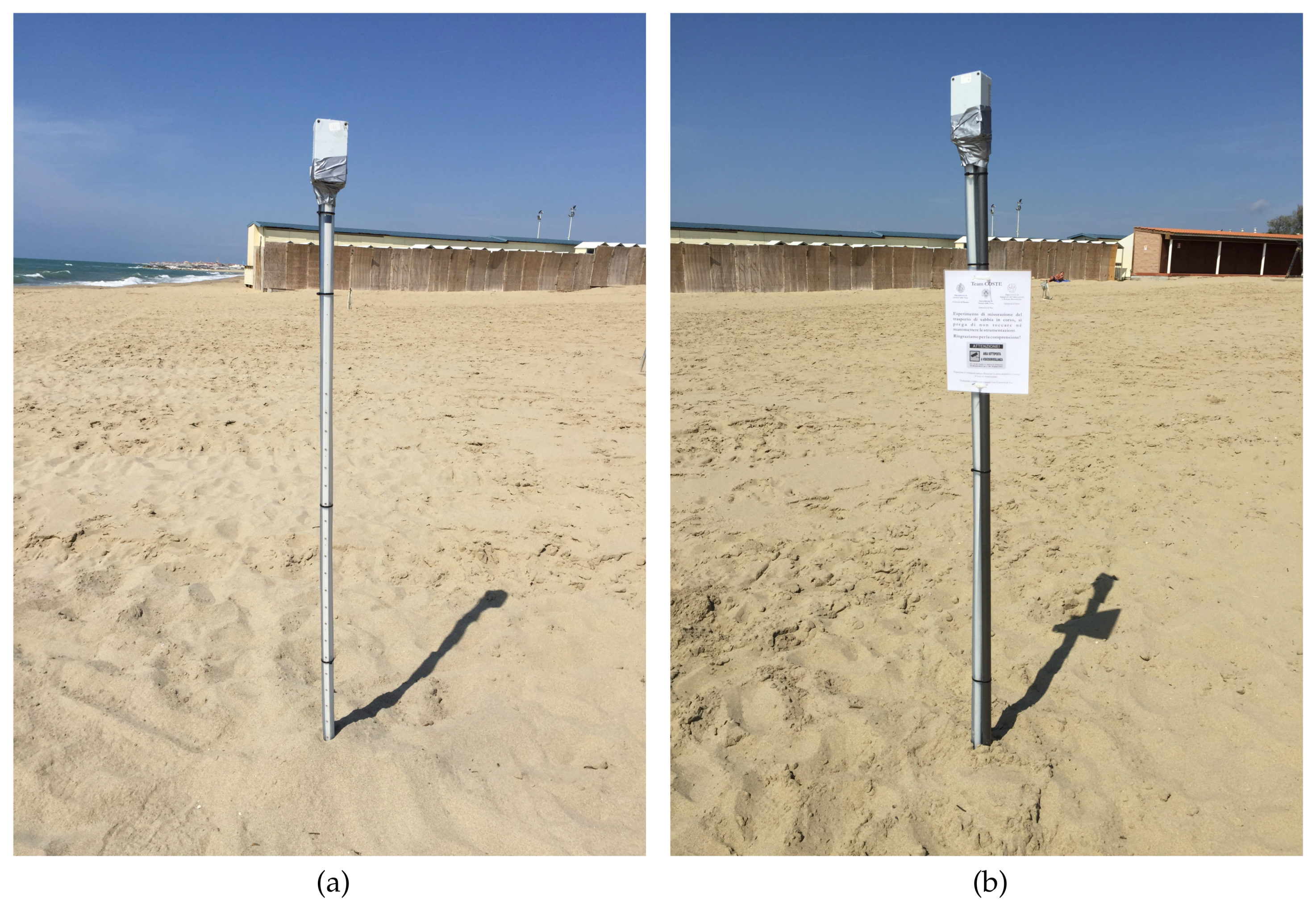
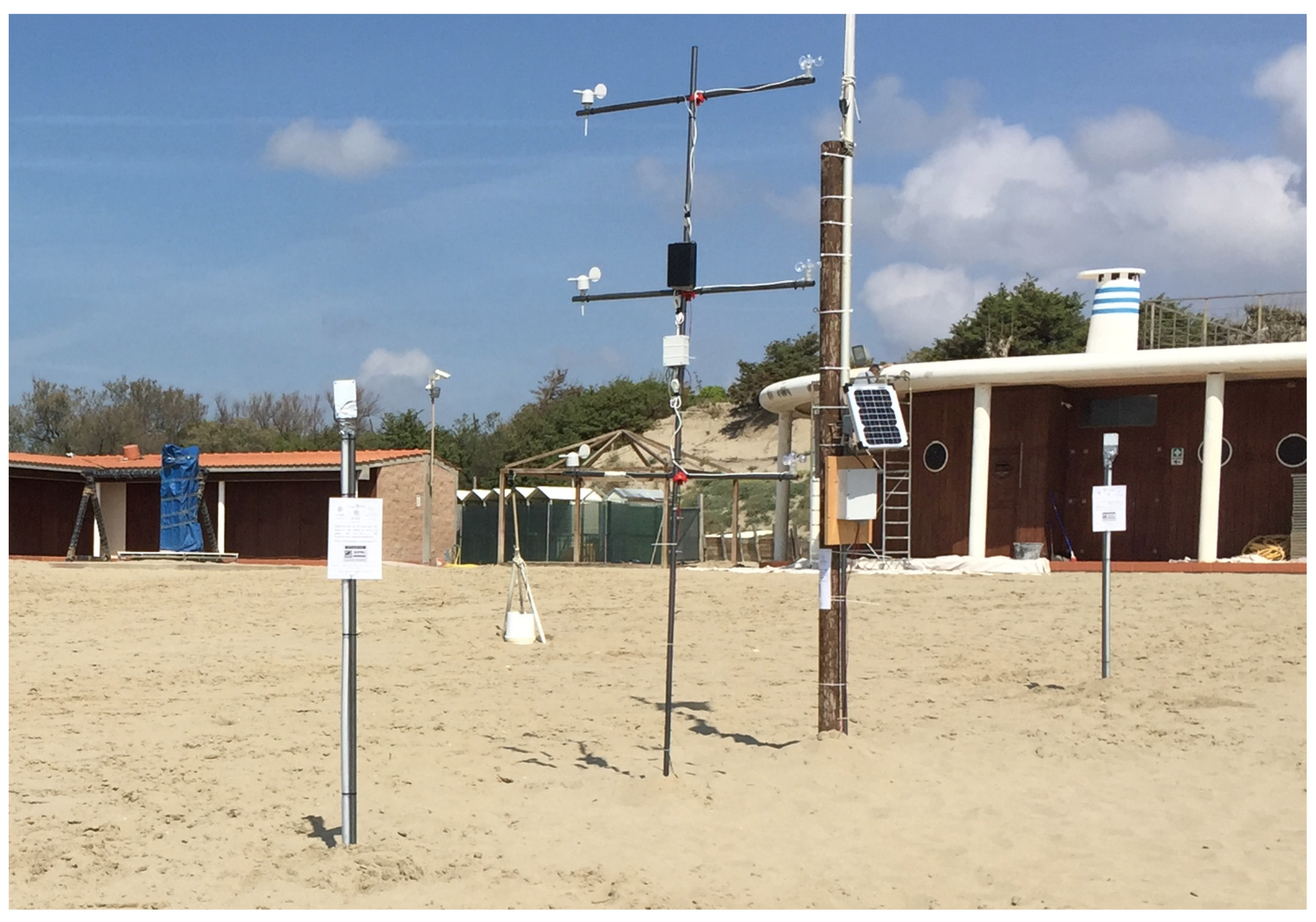
The second measurement campaign was carried out between 16 April 2017 and 22 April 2017 and saw the deployment of a two-node network configuration on the Marina di Tirrenia beach, near Pisa, Italy, close to a bathhouse that provided a video-surveillance service.
Figure 6 shows the two deployed sensor nodes, while
Figure 7 shows the overall network: between the two poles, it is possible to notice a structure for the measure of wind speed and direction, as well as the solar cell with the coordinator. The sample rate was set at one sample per hour: however, a small subset of the datasets went lost due to the weak GPRS network coverage on the site that turned into some short disconnection periods of the coordinator from the network. Nevertheless, the amount of received packets is however widely sufficient to define the sand level variation trend. In order to verify the correctness of the acquired data, they where checked manually daily directly on site by counting the number of emerging LDRs on the poles: this number allowed knowing the amount of buried LDRs that allowed checking the correctness of the value measured by the sensor. Each LDR count performed on site confirmed the accuracy of the measurement carried out by the sensors.
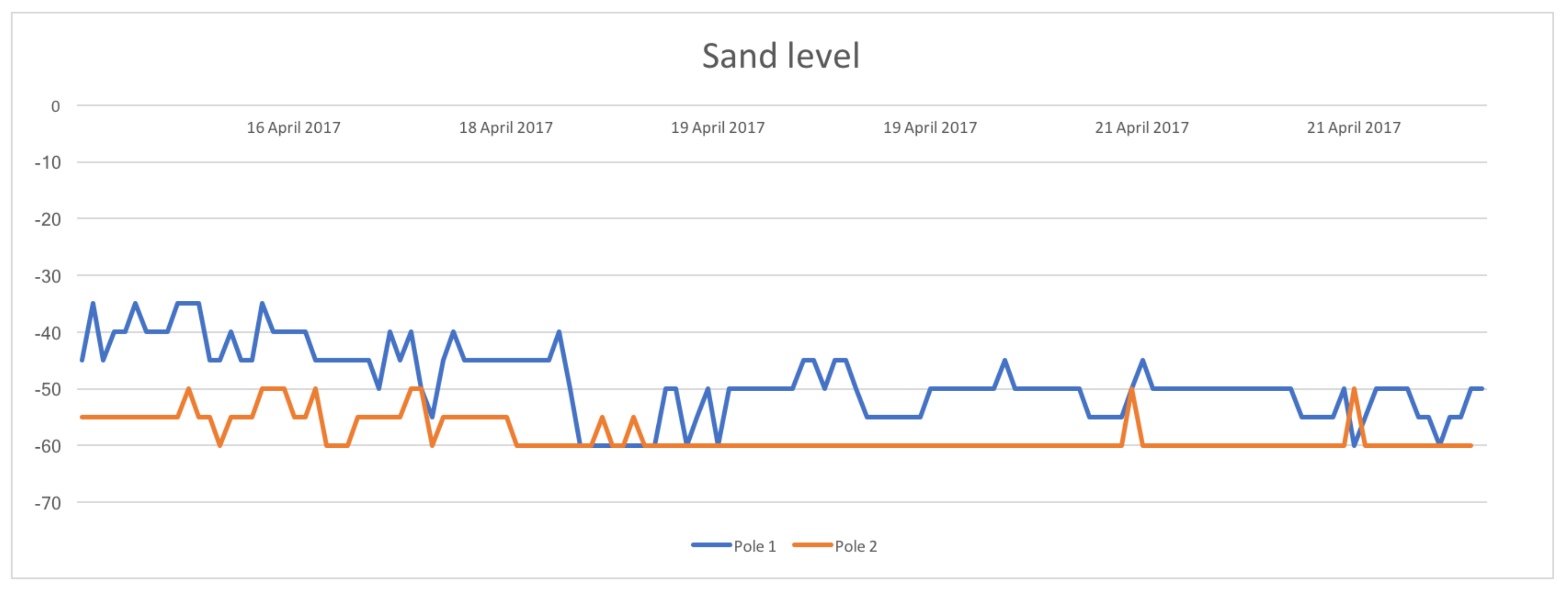
The trend of the data collected by the two sensor nodes for the whole measurement period can be seen in
Figure 8. The value range is between −60 cm and 60 cm assuming as zero the midpoint of the poles: indeed, once the system is fully operational, the poles are expected to be positioned half immersed in the sand, in order to measure both negative and positive variations of the sand level. However, for the test phase, in order to speed up the experimentation avoiding the digging of deep holes in the sand, the initial level was set at −45 cm for Pole 1 and at −55 cm for Pole 2. While the final values for the two poles are −50 cm for Pole 1 and −60 cm for Pole 2, it is however possible to conclude that during the test period, the sand level remained almost constant, as wind speed recorded during the same time span did not reach values able to consistently entrain and move sand particles of such a grain size.
While the system proved its operation following the field tests, some limitations can still be addressed. In particular: (i) measurements can only be carried out at fixed locations as the sensors are not free to move (this can be overcome by deploying as many nodes as possible to cover wide areas or by moving the nodes to different locations for every specific time span); (ii) the accuracy of the measurements is about 5 cm, which is lower relative to LiDAR surveys (this can be overcome by a reduction of the distance between consecutive sensors along the same pole); (iii) the system does not transmit the data if there is no GSM coverage in the area; (iv) the system does not record any measurement during the night (to overcome this limitation, the adoption of photoelectric barriers could be studied). Nevertheless, these limitations do not impact the overall effectiveness of the proposed solution.
9. Conclusions
The system described in this paper provides a low cost and low energy-consuming technique to measure sand level change in a sandy beach setting. In order to obtain these features, the design has been focused on a careful selection of components (counter, MUX and MOSFET) and on their circuital connections.
The best configuration for the XBee transmission module (the most demanding part, in terms of energy consumption) has been implemented by making it operate in sleep mode and by allowing a cyclic switching of the entire control logic. Considering that the developed system finds its more typical application in a scenario lacking other power sources, in the described way, it was possible to reach the prefixed objective, that is to guarantee for the sensor node, powered by simple AA batteries, as long a life time as possible.
By contrast, in order to achieve low costs and reduced power consumption, the sensor node has not been equipped with a data processing unit. This fact has influenced the choice of the network structure to be used. Two nodes at a time are activated for data acquisition and transmission to the network coordinator; then, the coordinator processes them and delivers the calculated values to the web server, allowing the user to visualize and control them in real time. Each successive pair of nodes is activated at a distance of about 2 min from the previous one, so as to allow the coordinator to carry out its work without interference. When fully operational, once all nodes have been activated, the system can work properly.
As sand transport processes are crucial to better define the sandy beach environment, the proposed system would offer the chance to collect a huge amount of data about real-time particle movement, which is an element that coastal managers often lack while discussing decisions to be made to manage coastal areas most appropriately.


