An Approach to Measuring Semantic Relatedness of Geographic Terminologies Using a Thesaurus and Lexical Database Sources

Abstract

In geographic information science, semantic relatedness is important for Geographic Information Retrieval (GIR), Linked Geospatial Data, geoparsing, and geo-semantics. But computing the semantic similarity/relatedness of geographic terminology is still an urgent issue to tackle. The thesaurus is a ubiquitous and sophisticated knowledge representation tool existing in various domains. In this article, we combined the generic lexical database (WordNet or HowNet) with the Thesaurus for Geographic Science and proposed a thesaurus–lexical relatedness measure (TLRM) to compute the semantic relatedness of geographic terminology. This measure quantified the relationship between terminologies, interlinked the discrete term trees by using the generic lexical database, and realized the semantic relatedness computation of any two terminologies in the thesaurus. The TLRM was evaluated on a new relatedness baseline, namely, the Geo-Terminology Relatedness Dataset (GTRD) which was built by us, and the TLRM obtained a relatively high cognitive plausibility. Finally, we applied the TLRM on a geospatial data sharing portal to support data retrieval. The application results of the 30 most frequently used queries of the portal demonstrated that using TLRM could improve the recall of geospatial data retrieval in most situations and rank the retrieval results by the matching scores between the query of users and the geospatial dataset.

1. Introduction

Semantic similarity relies on similar attributes and relations between terms, whilst semantic relatedness is based on the aggregate of interconnections between terms [1]. Semantic similarity is a subset of semantic relatedness: all similar terms are related, but related terms are not necessarily similar [2]. For example, “river” and “stream” are semantically similar, while “river” and “boat” are dissimilar but semantically related [3]. Similarity has been characterized as a central element of the human cognitive system and is understood nowadays as a pivotal concept for simulating intelligence [4]. Semantic similarity/relatedness measures are used to solve problems in a broad range of applications and domains. The domains of application include: (i) Natural Language Processing, (ii) Knowledge Engineering/Semantic Web and Linked Data [5], (iii) Information retrieval, (iv) Artificial intelligence [6], and so on. In this article, to accurately present our research, our study is restricted to semantic relatedness.

For geographic information science, semantic relatedness is important for the retrieval of geospatial data [7,8], Linked Geospatial Data [9], geoparsing [10], and geo-semantics [11]. For example, when some researchers tried to quantitatively interlink geospatial data [9], computing the semantic similarity/relatedness of the theme keywords of two geospatial data was required, such as the semantic similarity/relatedness of “land use” and “land cover” between a land use data set and a land cover data set. But computing the semantic similarity/relatedness of these geographic terminology is still an urgent issue to tackle.

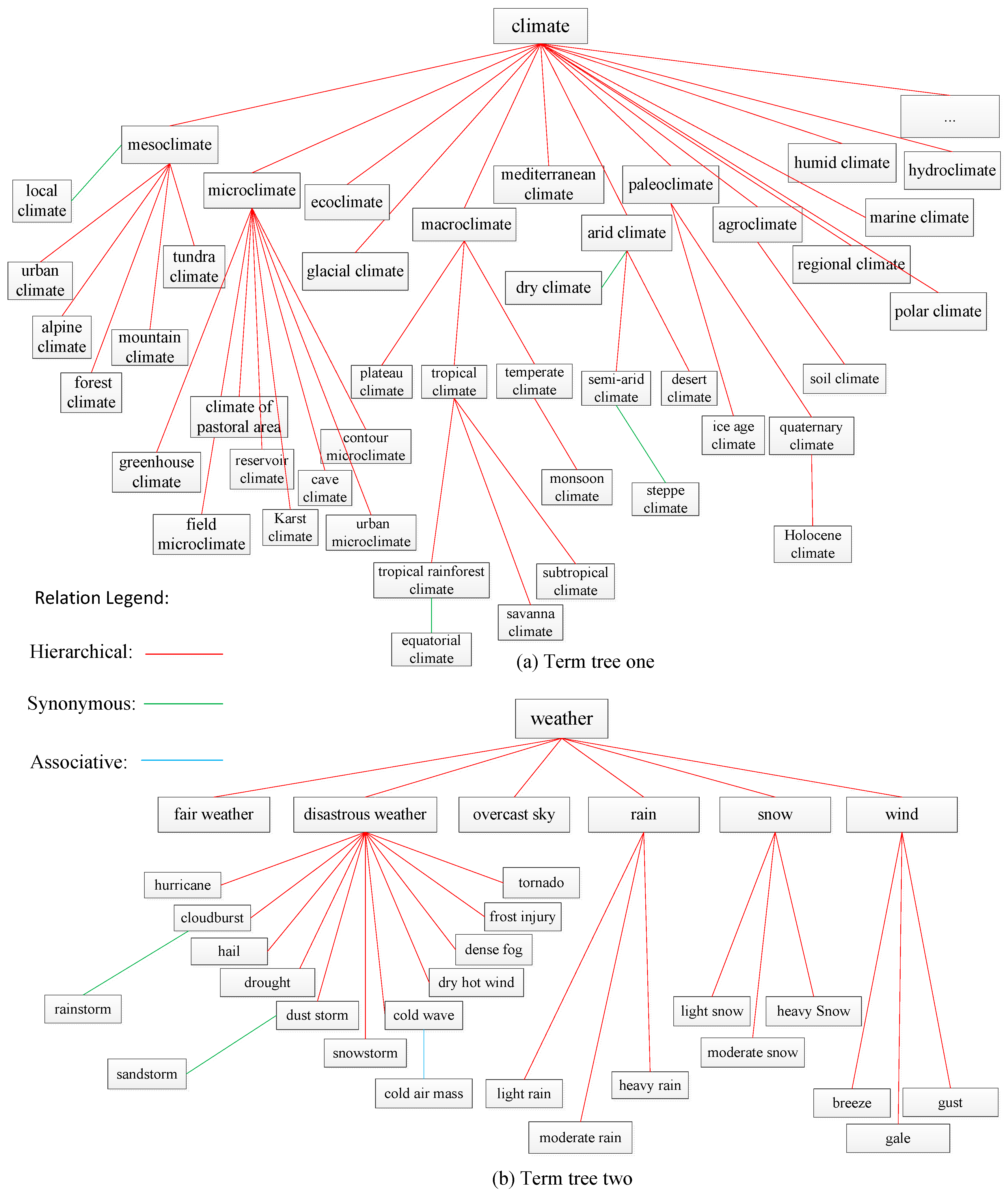
In the ISO standard, a thesaurus is defined as a “controlled and structured vocabulary in which concepts are represented by terms, organized so that relationships between concepts are made explicit, and referred terms are accompanied by lead-in entries for synonyms or quasi-synonyms” [12]. Actually, a thesaurus consists of numerous term trees. A term tree expresses one theme. In a term tree, there is a top term and other terms organized by three types of explicitly indicated relationships: (1) equivalence, (2) hierarchical and (3) associative. Equivalence relationships convey that two or more synonymous or quasi-synonymous terms label the same concept. Hierarchical relationships are established between a pair of concepts when the scope of one of them falls completely within the scope of the other. The associative relationship is used in “suggesting additional or alternative concepts for use in indexing or retrieval” and is to be applied between “semantically or conceptually” related concepts that are not hierarchically related [13,14]. For example, there are two term trees in Figure 1 whose top terms are “climate” and “weather” respectively. Terms are linked by three types of relationships; hierarchical relations are the main kind. A thesaurus is a sophisticated formalization of knowledge and there are several hundreds of thesauri in the world currently [13]. It has been used for decades for information retrieval and other purposes [13]. A thesaurus has also been used to retrieve information in GIScience [15], although the relationships it contains have not yet been analyzed quantitatively.

Given that there are only three types of relationships between terms in a thesaurus, it is relatively easy to build a thesaurus covering most of the terminologies in a discipline. So it is a practical choice to use a thesaurus to organize the knowledge of a discipline. Thesaurus for Geographic Sciences was a controlled and structured vocabulary edited by about 20 experts from the Institute of Geographic Sciences and Natural Resources Research (IGSNRR), Lanzhou Institute of Glaciology and Cryopedology (LIGC), and the Institute of Mountain Hazards and Environment (IMHE) of the Chinese Academy of Sciences. Over 10,800 terminologies of Geography and related domains were formalized in it. It was written in English and Chinese [16]. Its structure and modeling principles conformed to the international standards ISO-25964-1-2011 and its predecessor [12]. In this article, “the thesaurus” refers to the Thesaurus for Geographic Sciences hereafter.

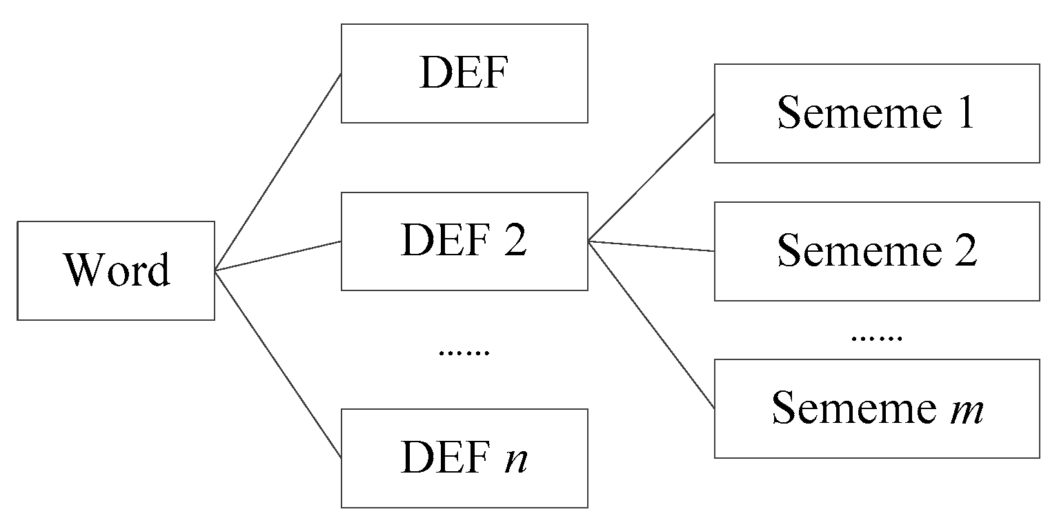
WordNet was a large generic lexical database of English which was devised by psychologists, linguists, and computer engineers from Princeton University [17]. In WordNet, nouns, verbs, adjectives and adverbs are grouped into sets of cognitive synonyms (synsets), each expressing a distinct concept. Synsets are interlinked by means of conceptual-semantic and lexical relations. In WordNet 3.0, there are 147,278 concept nodes in which 70% are nouns. There are a variety of semantic relations in WordNet, such as synonymy, antonymy, hypernymy, hyponymy and meronymy. The most common relations are hypernymy and hyponymy [18]. WordNet is an excellent lexicon to conduct word similarity computation. The main similarity measures for WordNet include edge counting-based methods [1], information theory-based methods [19], Jiang and Conrath’s methods [20], Lin’s methods [21], Leacock and Chodorow’s methods [22], Wu and Palmer’s methods [23], and Patwardhan and Pedersen’s vector and vectorp methods [24]. These measures obtain varying plausibility depending on the context and can be combined into ensembles to obtain higher plausibility [25]. WordNet is created by linguists, and it includes most of the commonly used concepts. Nevertheless, it does not cover most of the terminologies in a specific discipline. For example, in geography, the terminologies of “phenology”, “foredune”, “regionalization”, “semi-arid climate”, “periglacial landform”, and so on are not recorded in the WordNet database. Thus, when we want to tackle issues where semantic relatedness matters in a concrete domain, that is, in geography, WordNet fails. HowNet is a generic lexical database in Chinese and English. It was created by Zhendong Dong [26]. HowNet uses a markup language called KDML to describe the concept of words which facilitate computer processing [27]. There are more than 173,000 words in HowNet which are described by bilingual concept definition (DEF for short). A different semantic of one word has a different DEF description. A DEF is defined by a number of sememes and the descriptions of semantic relations between words. It is worth mentioning that a sememe is the most basic and the smallest unit which cannot be easily divided [28], and the sememes are extracted from about 6000 Chinese characters [29]. One word description in HowNet is shown in Figure 2.

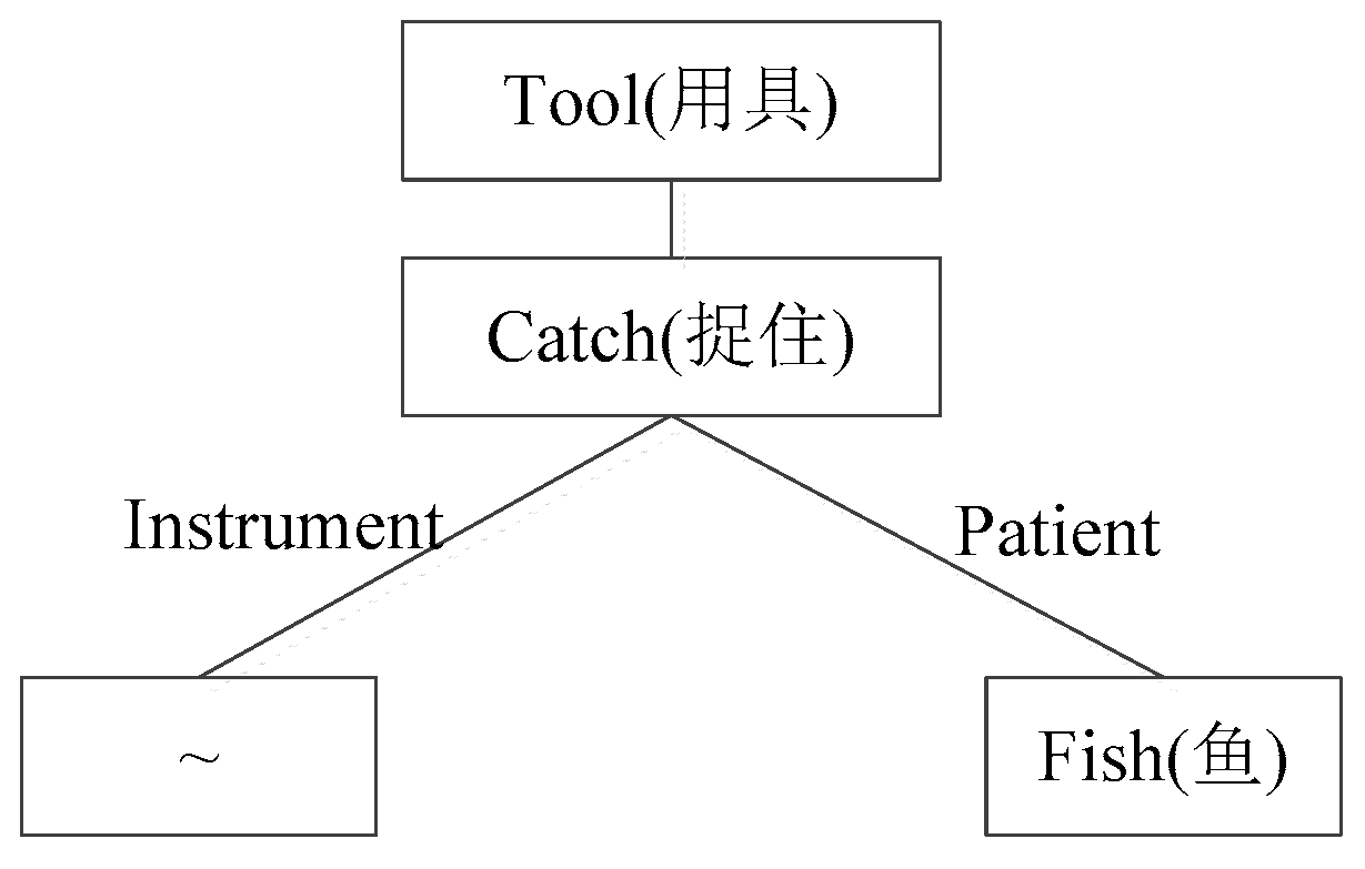
An example of one DEF of “fishing pole” can be described as follows:

DEF = {tool|用具:{catch|捉住: instrument = {~}, patient = {fish|鱼}}}.

In the example above, the words describing DEF, such as tool, catch, instrument, patient, and fish, are sememes. Then the description of DEF is a tree-like structure as shown in Figure 3. The relations between different sememes in DEF are described as a tree structure in the taxonomy document of HowNet.

To compute the similarity of Chinese words, Liu proposed an up-down algorithm on HowNet and achieved a good result [28]. Li proposed an algorithm based on the hierarchic DEF descriptions of words on HowNet [27]. Similar to WordNet, HowNet is also created by linguists and computer engineers. It includes most of the commonly used concepts and can not be used to compute the similarity of terminologies in a concrete domain.

In this article, we want to combine the generic lexical database with the thesaurus and present a new algorithm to compute the relatedness of any two terms in the Thesaurus for Geographic Science to realize the practical application of similarity/relatedness in geography for English and Chinese users.

The remainder of this article is organized as follows. Section 2 surveys relevant literature on semantic similarity or relatedness and issues that exist in semantic similarity and relatedness measures. Section 3 details TLRM, the proposed Thesaurus Lexical Relatedness Measure based on WordNet or HowNet and the Thesaurus for Geographic Sciences. Subsequently, an empirical evaluation of the measure is presented and discussed in Section 4. Then, we apply the proposed measure to geospatial data retrieval in Section 5. Lastly, we conclude with a discussion and a summary of directions for future research in Section 6 and Section 7.

2. Background

A semantic similarity/relatedness measure aims at quantifying the similarity/relatedness of terms as a real number, typically normalized in the interval $\in [0,1]$. There are numerous semantic similarity/relatedness measures proposed by researchers in different domains. These measures can be extensively categorized into two types: knowledge-based methods and corpus-based methods. Knowledge-based techniques utilize manually-generated artifacts as a source of conceptual knowledge, such as taxonomies or full-fledged ontologies [3]. Under a structuralist assumption, most of these techniques observe the relationships that link the terms, assuming, for example, that the distance is inversely proportional to the semantic similarity [1]. The corpus-based methods, on the other hand, do not require explicit relationships between terms and compute the semantic similarity of two terms based on their co-occurrence in a large corpus of text documents [30,31]. In terms of precision, the knowledge-based measures generally outperform the corpus-based ones [32].

In this article, we only review the literature of semantic similarity/relatedness measures based on the thesaurus knowledge sources or in the context of GIScience.

As a sophisticated and widely used knowledge formalization tool, the thesaurus has been used for computing the semantic similarity/relatedness of terms. For example, Qiu and Yu [33] devised a new thesaurus model and computed the conceptual similarity of the terms in a material domain thesaurus. In their thesaurus model, the terms with common super-class had been assigned a similarity value by domain experts. McMath et al. [34] compared several semantic relatedness (Distance) algorithms for terms in the medical and computer science thesaurus to match documents to the queries of users. Rada et al. [35] calculated the minimum conceptual distance for terms with hierarchical and non-hierarchical relations in EMTREE (The Excerpta Medica) thesaurus for ranking documents. Golitsyna et al. [36] proposed semantic similarity algorithms which were based on a set-theoretical model using hierarchical and associative relationships for terms in a combined thesaurus. Han and Li [37] quantified the relationships among the terms in a forestry thesaurus to compute the semantic similarity of forestry terms and built a semantic retrieval tool. Otakar and Karel [38] computed the similarity of the concept “forest” from seven different thesauri. Those approaches obtained nice results when applied to improve information retrieval processes. However, these methods remain incomplete and inaccurate when used to compute a semantic similarity/relatedness of terms. There are three aspects of issues in existing semantic similarity/relatedness measures based on a thesaurus. The first is that the measures can only compute the semantic similarity/relatedness of two terms which are in the same term tree of a thesaurus. The semantic similarity/relatedness of terms in different term trees cannot be computed or the value is assigned to 0 directly, which is not consistent with the facts. For example, in Figure 1, the relatedness of the terms of “macroclimate” and “polar climate”—which are in the same term tree—can be computed to 0.63 (assuming), but the semantic relatedness of “climate” and “fair weather” is assigned to 0 directly according to the existing method [37]. The second issue is that the researchers have not evaluated their semantic similarity/relatedness results because there are no suitable benchmarks available. The third issue is that some parameters of their algorithms have been directly obtained from previous research. Hence, they may not represent the optimal values for their specific situation. These issues have hampered the practical application of semantic similarity/relatedness, such as in a large-scale Geographic Information Retrieval System.

For geographic information science, several semantic similarity/relatedness measures have been proposed. For example, Rodríguez and Egenhofer [7] have extended Tversky’s set-theoretical ratio model in their Matching-Distance Similarity Measure (MDSM) [39]. Schwering and Raubal [40] proposed a technique to include spatial relations in the computation of semantic similarity. Janowicz et al. [11] developed Sim-DL, a semantic similarity measure for geographic terms based on description logic (DL), a family of formal languages for the Semantic Web. Sunna and Cruz [41] applied network-based similarity measures for ontology alignment. As such approaches rely on rich, formal definitions of geographic terminologies, it is almost impossible to build a large enough knowledge network required for a large-scale Geographic Information Retrieval System that covers most of the terminologies in the discipline of geography. Ballatore, Wilson, and Bertolotto [42] explored graph-based measures of semantic similarity on the OpenStreetMap (OSM) Semantic Network. They [43] have also outlined a Geographic Information Retrieval (GIR) system based on the semantic similarity of map viewport. In 2013, Ballatore et al. [3] proposed a lexical definition semantic similarity approach using paraphrase-detection techniques and the lexical database WordNet based on volunteered lexical definitions which were extracted from the OSM Semantic Network. More recently, Ballatore et al. [10] proposed a hybrid semantic similarity measure, the network-lexical similarity measure (NLS). The main limitation of these methods lies in the lack of a precise context for the computation of the similarity measure [10], because the crowdsourcing geo-knowledge graph of the OpenStreetMap Semantic Network is not of high quality intrinsically in terms of knowledge representation and has limitations in coverage.

Therefore, in this article, we use the thesaurus as an expert-authored knowledge base which is relatively easy to construct, utilize a generic lexical database (hereafter, the generic lexical database refers to WordNet or HowNet) to interlink the term trees in the thesaurus and adopt a knowledge-based approach to compute the semantic relatedness of terminologies. Furthermore, a new baseline for the evaluation of the relatedness measure of geographic terminologies will be built and used to evaluate our measure. In this way, we can reliably compute the relatedness of any two terms recorded in the thesaurus by leveraging quantitative algorithms. In the next section, we will first provide details regarding the semantic relatedness algorithms.

3. Thesaurus Lexical Relatedness Measure

3.1. Related Definition

Definition 1: A descriptor is a preferred term in formal expression [44]. For example, “arid climate” is a descriptor while “dry climate” is not although they represent the same concept in Figure 1. Generally, descriptors form the hierarchical and associative relationships in a thesaurus, but in this article, we define descriptors as preferred terms which are used to form the hierarchical relationships in a thesaurus. As shown in Figure 1, all the terms linked by red lines are descriptors.

Definition 2: In a thesaurus, a concept tree is a tree-like hierarchical structure of artifacts (denoted as $T$ in this article) that is consisted of all descriptors about a theme. The top term of the tree is $O$. The descriptor in the tree $T$ is denoted as $C$ (A node or descriptor node in the tree also refers to a descriptor). The top term $O$ is also denoted as $C_0$. $C_i$ is the i-th descriptor by a hierarchical traversal in $T$ starting from the top term. All the ancestor nodes of $C$ in $T$ constitute the ancestor descriptor set $A(C)$. All the child nodes of $C$ constitute the child descriptor set $L(C)$. If at least one term $W$ who is associated to the descriptor $C$ exists, the descriptor $C$ is the associative descriptor of $W$ ($W$ is not a descriptor). The depth of the top term $O$ is 1. For example, in Figure 1, for the first term tree, all the terms linked by red lines and their relationships constitute a concept tree, and the “climate” is the top term. For the descriptor “tropical climate”, its ancestor descriptor set $A(C)=\{“\mathrm{climate}”,“\mathrm{macroclimate}”\}$ and child descriptor set $L(C)=\{“\mathrm{tropical}\mathrm{rainforest}\mathrm{climate}”,“\mathrm{savanna}\mathrm{climate}”,“\mathrm{subtropical}\mathrm{climate}”\}$.

Definition 3: In a concept tree, the path formed by the least edges between two descriptors is called the shortest path between the two descriptors. The number of edges of the path is called the minimum path length.

Definition 4: In a concept tree $T$, if the node $R$ is the lowest node that has both descriptor A and B as descendants, $R$ is called the least common subsumer of A and B, denoted as $R(A,B)$ or $R$ (we define each node to be a descendant of itself).

Definition 5: The depth of a descriptor represents the number of levels of hierarchy from the node to the top term in a concept tree. The depth of two or more descriptors is the depth of their least common subsumer. For example, in Figure 1, the depth of “plateau climate” and “subtropical climate” is 2 while the depth of “subtropical climate” is 4.

Definition 6: In a concept tree $T$, the number of leaf nodes in the subtree of descriptor $C$ is called the semantic coverage of $C$, denoted as $SCover(C)$. For example, the semantic coverage of “paleoclimate” is 2 and its leaf nodes are “ice age climate” and “Holocene climate” in first term tree of Figure 1.

Definition 7: In a concept tree $T$ which contains $n$ descriptor nodes, the node $C_i$ can be represented as a vector $C_i=(V_{i,1},V_{i,2},\dots ,V_{i,n})$, $V_{i,j}(i=1,2,\dots ,n;j=1,2,\dots ,n)$. The vector is called the local semantic density vector of descriptor $C_i$. The value of $V_{i,j}$ is defined as follows [37]:

$$V_{i,j}=\{\begin{array}{l}1,C_j\subset \{C_i,L(C_i)\}\\ \frac{SCover(C_i)}{SCover(C_j)},C_j\subset \{A(C_i)\}\\ 0,else\end{array}$$

(1)

From the definitions above, it can be found that a concept tree is the skeleton of the term tree in a thesaurus. There are only hierarchical relationships in a concept tree but there are three kinds of relationships in a term tree.

3.2. Algorithms

Set the two terms to be determined for relatedness as $C_1$ and $C_2$ and their relatedness to be $Sim(C_1,C_2)$. In this article, we consider that the relatedness of the exactly same terms is 1, and the interval of relatedness is [0,1]. We will determine $Sim(C_1,C_2)$ according to the locations of $C_1$ and $C_2$ in the term tree.

3.2.1. $C_1$ and $C_2$ Are in the Same Term Tree

If $C_1$ and $C_2$ are in the same term tree, there are four kinds of path linking them, namely, synonymous or equivalent path, hierarchical path, associative path, and compound path. A synonymous or equivalent path means that the relationship between $C_1$ and $C_2$ is synonymous or equivalent. A hierarchical path means that $C_1$ and $C_2$ are in the same concept tree. An associative path means that the relationship between $C_1$ and $C_2$ is associative. A compound path means that $C_1$ and $C_2$ are linked by at least two kinds of relationships. For example, as shown in Figure 1, for the second term tree, the path between “cloudburst” and “rainstorm” is a synonymous path, the path between “cloudburst” and “cold wave” is a hierarchical path, the path between “cold wave” and “cold air mass” is an associative path, and the path between “rainstorm” and “cold air mass” is a compound path. We will determine $Sim(C_1,C_2)$ from these cases:

1. Equivalent or synonymous path

In a thesaurus, synonyms are the terms that denote the same concept and are interchangeable in many contexts, so we propose that the relatedness of $Sim(C_1,C_2)$ between $C_1$ and $C_2$ in the relation is equal to 1, namely,

$$Sim(C_1,C_2)=SimS(C_1,C_2)=1$$

(2)

where $SimS$ refers to the relatedness of two terms in an equivalent or synonymous relationship.

2. Hierarchical path

If $C_1$ and $C_2$ are nodes in a concept tree $T$ (Please note that that the relationship between $C_1$ and $C_2$ may not be parent and child), the relatedness of $Sim(C_1,C_2)$ is a function of the characteristics of minimum path length, depth, and local semantic density of nodes, as follows [6]:

$$Sim(C_1,C_2)=SimH(C_1,C_2)=f(l,h,d)$$

(3)

where, $l$ is the minimum path length between $C_1$ and $C_2$, $h$ is the depth of $C_1$ and $C_2$ in the concept tree, and $d$ is the local semantic density of $C_1$ and $C_2$.

We assume that (3) can be rewritten to three independent functions as:

$$Sim(C_1,C_2)=SimH(C_1,C_2)=f(f_1(l),f_2(h),f_3(d))$$

(4)

$f_1$, $f_2$, $f_3$ are transfer functions of minimum path length, depth, and local semantic density, respectively. That is to say, the influence factors of path length, depth, and local semantic density of relatedness are independent. The independence assumption in (4) enables us to investigate the contribution of the individual factor to the overall relatedness through a combination of them.

According to Shepard’s law [45], exponential-decay function is a universal law of stimulus generalization for psychological science. We set $f_1(l)$ in (4) to be a monotonically decreasing function of $l$:

$$f_1(l)=e^{-\theta l}$$

(5)

where $\theta$ is a constant.

According to Definition 5, the depth of $C_1$ and $C_2$ is derived by counting the number of levels of hierarchy from the top term to their least common subsumer in the concept tree. In a concept tree, terms at the upper layers have more general concepts and less semantic between terms than terms at lower layers [6]. This behavior must be taken into account in calculating $Sim(C_1,C_2)$. We therefore need to scale down $Sim(C_1,C_2)$ for the least common subsumer of $C_1$ and $C_2$ at upper layers and scale up $Sim(C_1,C_2)$ for that at lower layers. Moreover, the relatedness interval is finite, say [0,1], as stated earlier. As a result, $f_2(h)$ should be a monotonically increasing function with respect to depth $h$. To satisfy these constraints, we set $f_2(h)$ as [6]:

$$f_2(h)=\frac{e^{\beta h}-e^{-\beta h}}{e^{\beta h}+e^{-\beta h}}$$

(6)

where $\beta >0$ is a smoothing factor.

The concept vector model generalizes standard representations of relatedness concepts in terms of a tree-like structure. In the model, a concept node in a hierarchical tree is represented as a concept vector according to its relevant node density [46]. The relatedness of two concepts is obtained by computing the cosine similarity of their vectors [46]. In this article, the local semantic density vector of a descriptor is a concept vector. However, the relatedness measure based on concept vectors is effective only when there is an overlap among the components of the two vectors. When there is no overlap in the vectors, the relatedness score is 0. For example, for the descriptors “forest climate” and “mountain climate” in the first term tree of Figure 1, the cosine similarity of their concept vectors is 0. It is obvious that the two terms’ similarity/relatedness is not 0. Hence, we deem that the local semantic density influences the total relatedness of the two terms to some extent. We set $f_3(d)$ as:

$$f_3(d)=\delta +(1-\delta )\cdot \frac{\stackrel{\rightharpoonup }{C_1}·\stackrel{\rightharpoonup }{C_2}}{|\stackrel{\rightharpoonup }{C_1}||\stackrel{\rightharpoonup }{C_2}|}$$

(7)

where $\delta$ is a constant and $0<\delta \le 1$. $\stackrel{\rightharpoonup }{C_1}$ and $\stackrel{\rightharpoonup }{C_2}$ are the local semantic density vectors of descriptor $C_1$ and $C_2$, deriving from Definition 7.

Hence, the relatedness of $C_1$ and $C_2$ is as follows:

$$Sim(C_1,C_2)=SimH(C_1,C_2)=f_1(l)\times f_2(h)\times f_3(d)$$

(8)

where $SimH$ refers to the relatedness of two terms in a concept tree.

3. Associative path

If $C_1$ is the associative descriptor of $W_1$, we deem that the depth of $C_1$ and $W_1$ is the depth of $C_1$ in this article and the depth of $C_1$ will influence the semantic relatedness obviously (Because, in a concept tree, terms at the upper layers have more general concepts and less semantic between terms than terms at lower layers [6]). In addition, the number of alternative concepts that are associative to $C_1$ also influences the semantic relatedness [37]. We denote the number of alternative concepts as the semantic density. Hence, the semantic relatedness of $Sim(C_1,W_1)$ is a function of the characteristics of depth and semantic density [37] and is defined as follows:

$$Sim(C_1,W_1)=SimR(C_1,W_1)=g_1(h)\times g_2(n)$$

(9)

where $g_1(h)$ and $g_2(n)$ are transfer functions of depth, and semantic density, respectively. Similar to Equation (6), we get $g_1(h)$ with a different smoothing factor:

$$g_1(h)=\frac{e^{\epsilon h}-e^{-\epsilon h}}{e^{\epsilon h}+e^{-\epsilon h}},$$

(10)

and

$$g_2(n)=e^{-\gamma n}$$

(11)

where $\gamma$, $\epsilon$ are constants, $h$ is the depth of the descriptor of $C_1$, and $n$ is the number of concepts that are associative to the descriptor $C_1$.

4. Compound path

If $C_1$ and $C_2$ are linked by different relationships in a term tree, we will divide their shortest path into several pure parts, compute the relatedness of each of the pure parts using the algorithms proposed above, and then multiply these relatedness. For example, in Figure 1, the relatedness of “sandstorm” and “cold air mass” is the product of $SimS(“\mathrm{sandstorm}”,“\mathrm{dust}\mathrm{storm}”)$, $SimH(“\mathrm{dust}\mathrm{storm}”,“\mathrm{cold}\mathrm{wave}”)$, and $SimR(“\mathrm{cold}\mathrm{wave}”,“\mathrm{cold}\mathrm{air}\mathrm{mass}”)$ which are computed by Equations (2), (8) and (9) respectively.

3.2.2. $C_1$ and $C_2$ Are in Different Term Trees

If $C_1$ and $C_2$ are in different term trees, set the top term of $C_1$ as $O_1$ and the top term of $C_2$ as $O_2$. We divide the relatedness of $Sim(C_1,C_2)$ into three parts that are the relatedness of $Sim(C_1,O_1)$, $Sim(O_1,O_2)$, and $Sim(C_2,O_2)$, and we obtain:

$$Sim(C_1,C_2)=Sim(C_1,O_1)\times Sim(O_1,O_2)\times Sim(C_2,O_2)$$

(12)

where $Sim(C_1,O_1)$ and $Sim(C_2,O_2)$ are computed by the algorithms in Section 3.2.1. $Sim(O_1,O_2)$ is computed by the following methods based on WordNet or HowNet. Given that $O_1$ and $O_2$ are top terms and we know that terms at upper layers of hierarchical semantic nets have more general concepts [6], the top terms are general concepts, which—or segments of which—can be found in the WordNet or HowNet lexical database. For example, in Figure 1, the terms “climate” and “weather” can be found in WordNet lexical databases (The corresponding Chinese terms are “气候” and “天气” which can be found in HowNet lexical databases), while the term “frozen ground” (“冻土” for Chinese), which is the top term of another term tree in Thesaurus for Geographic Science, cannot be found in WordNet directly (“冻土” also can not be found in HowNet databases directly), but its segments, namely, “frozen” and “ground”, can be found in WordNet (The segments of “冻土” are “冻” and “土” which can be found in HowNet for Chinese). (Actually, we looked up the 389 top terms of the Thesaurus for Geographic Science in WordNet and HowNet. Most of them can be found in WordNet or HowNet directly. The remainders are compound words and their segments can all be found in WordNet and HowNet). The relatedness of top terms from different term trees can be computed by the following methods:

Segment $O_1$ as $\{t_{11},t_{12},\dots ,t_{1n}\}$ and $O_2$ as $\{t_{21},t_{22},\dots ,t_{2m}\}$ where $t_{ij}$ is a single word which can be find in WordNet or HowNet databases. The term set of $\{t_{11},t_{12},\dots ,t_{1n}\}$ contributes to conveying the meaning of $O_1$. To represent the geographic terminology $O_1$ in a semantic vector space, we define a vector $\stackrel{\rightharpoonup }{O_1}=\{t_{11},t_{12},\dots ,t_{1n}\}$, whose components are the segmented words $\{t_{11},t_{12},\dots ,t_{1n}\}$, the same as $\stackrel{\rightharpoonup }{O_2}=\{t_{21},t_{22},\dots ,t_{2m}\}$. If $O_1$ or $O_2$ is a single word, there is only one element in $\stackrel{\rightharpoonup }{O_1}$ or $\stackrel{\rightharpoonup }{O_2}$ correspondingly.

Having constructed the semantic vectors $\stackrel{\rightharpoonup }{O_1}$ and $\stackrel{\rightharpoonup }{O_2}$, it is possible to compute the vector-to-vector relatedness $si{m}_v$. An asymmetric relatedness measure of semantic vectors $si{m}_v^{\prime }(\stackrel{\rightharpoonup }{O_1},\stackrel{\rightharpoonup }{O_2})$ can be formalized as follows:

$$si{m}_v^{\prime }(\stackrel{\rightharpoonup }{O_1},\stackrel{\rightharpoonup }{O_2})=\frac{{\displaystyle \sum _{i=1}^{|\stackrel{\rightharpoonup }{O_1}|}\widehat{s}(t_{1i},\stackrel{\rightharpoonup }{O_2}})}{|\stackrel{\rightharpoonup }{O_1}|}, si{m}_v^{\prime }(\stackrel{\rightharpoonup }{O_2},\stackrel{\rightharpoonup }{O_1})=\frac{{\displaystyle \sum _{i=1}^{|\stackrel{\rightharpoonup }{O_2}|}\widehat{s}(t_{2i},\stackrel{\rightharpoonup }{O_1}})}{|\stackrel{\rightharpoonup }{O_2}|}, si{m}_v^{\prime }(\stackrel{\rightharpoonup }{O_1},\stackrel{\rightharpoonup }{O_2})\in [0,1]$$

(13)

where $|\stackrel{\rightharpoonup }{O_1}|$ and $|\stackrel{\rightharpoonup }{O_2}|$ are the dimensions of the vector $\stackrel{\rightharpoonup }{O_1}$ and $\stackrel{\rightharpoonup }{O_2}$ respectively; the function $\widehat{s}$ corresponds to the maximum semantic relatedness score between the term $t_{ij}$ and the vector $\stackrel{\rightharpoonup }{O}$ based on the algorithm presented by Corley and Mihalcea [47]. That is,

$$\widehat{s}(t_{1i},\stackrel{\rightharpoonup }{O_2})=Max\{sim(t_{1i},t_{21}),sim(t_{1i},t_{22}),\dots ,sim(t_{1i},t_{2m})\}$$

(14)

where $sim(t_{1i},t_{2j})$ is a similarity between two words computed by the WordNet-based or HowNet-based method. In this article, we use Patwardhan and Pedersen’s vector method as the WordNet-based method to compute $sim(t_{1i},t_{2j})$ for English terms, because this measure outperforms other measures in terms of precision of word relatedness computation according to the report [24]. We use the up-down algorithm proposed by Liu [28] as the HowNet-based method to compute $sim(t_{1i},t_{2j})$ for Chinese terms. A symmetric measure $si{m}_v\in [0,1]$ can be easily obtained from $si{m}_v^{\prime }$ as

$$Sim(O_1,O_2)=si{m}_v(\stackrel{\rightharpoonup }{O_1},\stackrel{\rightharpoonup }{O_2})=\frac{si{m}_v^{\prime }(\stackrel{\rightharpoonup }{O_1},\stackrel{\rightharpoonup }{O_2})+si{m}_v^{\prime }(\stackrel{\rightharpoonup }{O_2},\stackrel{\rightharpoonup }{O_1})}{2}$$

(15)

Based on the algorithms above, we can compute the semantic relatedness of any two terminologies in the thesaurus. What we should note is that the algorithms have not been provided with values for the following parameters: $\theta$, $\beta$, $\delta$, $\epsilon$, $\gamma$. In the next section, we will determine the values of these parameters and evaluate the precision of the proposed measure.

4. Evaluation

The quality of a computational method for computing term relatedness can only be established by investigating its performance against human common sense [6]. To evaluate our method, we have to compare the relatedness computed by our algorithms against what experts rated on a benchmark terminology set. There are many benchmark data sets used to evaluate similarity/relatedness algorithms, for example, that of Miller and Charles [48], called M & C, that of Rubenstein and Goodenough [49], called R & G, that of Finkelstein et al. [50], called WordSimilarity-353, and that of Nelson et al. [51], called WordSimilarity-1016, in Natural Language Processing. In the areas of GIScience, Rodríguez and Egenhofer [7] collected similarity judgements about geographical terms to evaluate their Matching-Distance Similarity Measure (MDSM). Ballatore et al. [2] proposed GeReSiD as a new open dataset designed to evaluate computational measures of geo-semantic relatedness and similarity. Rodríguez and Egenhofer’s similarity evaluation datasets and GeReSiD are gold standards for the evaluation of geographic term similarity or relatedness measures. However, their terms mostly regard geographic entities, such as the “theater” and “stadium”, “valley” and “glacier”. They are not very suitable to evaluate the relatedness of geography terminologies, such as “marine climate” and “polar climate”. We call the Rodríguez and Egenhofer’s similarity evaluation data set and GeReSiD geo-semi-terminology evaluation data sets. Now we have to build a geo-terminology evaluation dataset that can be used to evaluate the relatedness measure of geography terminology.

This section presents the Geo-Terminology Relatedness Dataset (GTRD), a dataset of expert ratings that we have developed to provide a ground truth for assessment of the computational relatedness measurements.

4.1. Survey Design and Results

Given that terminologies deal with professional knowledge, we should conduct the survey with geography experts. The geographic terms included in this survey are taken from the Thesaurus for Geographic Science. First, we selected term pairs from a term tree, which were the combinations of terms with different relationships, distances, depths, and local semantic density. Then, other term pairs were selected from different term trees whose top terms were of different relatedness ranging from very high to very low, which were also combinations of terms with different relationships, distances, depths, and local semantic density. We eventually selected a set of 66 terminology pairs for the relatedness rating questionnaire which could be logically divided into two parts: 33 pairs of the data set were the combinations of terms with different characteristics from the same and different term trees, and the other 33 pairs were the combinations of terms with duplicate characteristics compared to the former. The 33 terminology pairs of the data set were assembled by the following components: 8 high-relatedness pairs, 13 middle-relatedness pairs, and 12 low-relatedness pairs.

We sent emails attaching the questionnaires to 167 geography experts whose research interests included Physical Geography, Human Geography, Ecology, Environmental Science, Pedology, Natural Resources, and so on. The experts were asked to judge the relatedness of the meaning of 66 terminology pairs and rate them on a 5-point scale from 0 to 4, where 0 represented no relatedness of meaning and 4 perfect synonymy or the same concept. The ordering of the 66 pairs was randomly determined for each subject.

Finally, we received 53 responses, among which, two experts did not complete the task and another two subjects provided incorrect ratings, that is the highest rating score offered was 5. These four responses were discarded. In order to detect unreliable and random answers of experts, we computed the Pearson’s correlation coefficient between every individual subject and the mean response value. Pearson’s correlation coefficient, also referred to as the Pearson’s r or bivariate correlation, is a measure of the linear correlation between two variables X and Y. Generally, the value of [0.8,1] of Pearson’s r means a strong positive correlation [52], so the responses with Pearson’s correlation coefficient <0.8 were also removed from the data set in order to ensure the high reliability of the relatedness gold standard. Eight experts’ judgments were removed because of a lower Pearson’s correlation coefficient. Finally, 41 expert responses were utilized as the data source for our relatedness baseline.

Intra-Rater Reliability (IRR) refers to the relative consistency in ratings provided by multiple judges of multiple targets [53]. In contrast, Intra-Rater Agreement (IRA) refers to the absolute consensus in scores furnished by multiple judges for one or more targets [54]. Following LeBreton and Senter [55] who recommended using several indices for IRR and IRA to avoid the bias of any single index, the following indices for IRA and IRR were selected: the Pearson’s r [56], the Kendall’s $\tau$ [57], the Spearman’s $\rho$ for IRR; the Kendall’s $W$ [58], James, Demaree and Wolf’s $r_{WG(J)}$ [59] for IRA.

Table 1. Indices of Intra-Rater Reliability (IRR) and Intra-Rater Agreement (IRA) for the Geo-Terminology Relatedness Dataset (GTRD).

Index Type	Index Name	Minimum	Median	Max	Means
IRR	Pearson’s $r$	0.816	0.86	0.922	0.86
	Spearman’s $\rho$	0.797	0.858	0.925	0.858
	Kendall’s $\tau$	0.657	0.734	0.807	0.731
Index Type	Index Name	Value	Index type	Index name	Value
IRA	Kendall’s $W$	0.731	IRA	$r_{WG(J)}$	0.927

p < 0.001.

shows the values of the indices of IRR and IRA.

The indices of IRR and IRA in Table 1 indicate that the GTRD possesses a high reliability and is in agreement among geography experts. The correlation is satisfactory, and is better than analogous surveys [2].

Given the set of terminology pairs and expert ratings, we computed the mean ratings of the 41 experts, and normalized them in the interval of [0,1] as relatedness scores (https://github.com/czgbjy/GTRD). The GTRD is shown in

Table 2. Inversion pairs of GTRD.

Term One	Term Two	Relatedness
oasis city	oasis city	1
tropical rainforest climate	equatorial climate	0.8720
city	cities and towns	0.8598
plateau permafrost	frozen soil	0.7805
cold wave	cold air mass	0.7744
geographical environment	environment	0.7134
highway transportation	transportation	0.7073
semi-arid climate	steppe climate	0.7073
climate	weather	0.6890
dairy Industry	food industry	0.6829
processing industry	light industry	0.6646
coal industry	heavy industry	0.6280
ecological environment	water environment	0.5915
alpine desert soil	subalpine soil	0.5732
low productive soil	soil fertility	0.5671
automobile industry	basic industry	0.5122
social environment	external environment	0.4756
plateau climate	ecological environment	0.4268
technique intensive city	small city	0.4146
feed industry	sugar industry	0.3902
fair weather	overcast sky	0.3902
Mediterranean climate	semi-arid environment	0.3415
gas industry	manufacturing industry	0.2988
agroclimate	natural landscape	0.2805
petroleum industry	aluminum industry	0.25
textile industry	shipbuilding industry	0.25
monsoon climate	meadow cinnamon soil	0.2134
quaternary climate	steppe landscape	0.1646
humid climate	dust storm	0.1585
marine environment	soil	0.1098
ecoclimate	science city	0.0549
marine climate	pipeline transportation	0.0366
desert climate	inland water transportation	0.0305

and

Table 3. The relatedness generated by the thesaurus–lexical relatedness measure (TLRM) and expert ratings on evaluation pairs.

Term One	Term Two	GTRD	TLRM (WordNet)	TLRM (HowNet)
waterway transportation	waterway transportation	1	1	1
port city	harbor city	0.9085	1	1
transportation	communication and transportation	0.8293	1	1
near shore environment	coastal environment	0.7805	0.7596	0.7301
near shore environment	sublittoral environment	0.7805	0.5776	0.5302
iron and steel industry	metallurgical industry	0.7256	0.763	0.7444
cultural landscape	landscape	0.6707	0.5851	0.5633
cold wave	disastrous weather	0.6524	0.7623	0.7416
agricultural product processing industry	industry	0.6098	0.4535	0.4473
gray desert soil	brown desert soil	0.6037	0.5776	0.5302
marine environment	geographical environment	0.5976	0.5902	0.5861
tropical soil	subtropical soil	0.5732	0.5776	0.5302
alpine meadow soil	chestnut soil	0.4634	0.3508	0.3514
power industry	mechanical industry	0.4512	0.4502	0.4316
hydroclimate	agricultural environment	0.4146	0.1664	0.3341
marine transportation	air transportation	0.3780	0.4502	0.4316
arid climate	paleoclimate	0.3780	0.5776	0.5303
environment	disastrous weather	0.3659	0.1301	0.0335
marine climate	cold air mass	0.3171	0.0847	0.2994
desert soil	permafrost	0.3171	0.5038	0.1676
global environment	human landscape	0.2805	0.1651	0.3003
tropical climate	coastal environment	0.2744	0.0623	0.1574
computer industry	building material industry	0.2317	0.3508	0.3514
climate	city	0.2134	0.1463	0.2087
city	textile industry	0.2012	0.1841	0.0661
regional climate	megalopolis	0.1829	0.0497	0.0641
water environment	steppe landscape	0.1829	0.1005	0.2018
temperate climate	superaqual landscape	0.1707	0.1120	0.1574
glacial climate	cinnamon soil	0.1402	0.1480	0.2042
semi-arid environment	subaqual landscape	0.1037	0.0603	0.1258
Holocene climate	coastal transportation	0.0366	0.0193	0.0152
polar climate	mining industry	0.0244	0.0583	0.0516
desert climate	labor intensive industry	0.0061	0.0353	0.0337

.

4.2. Determination of Parameters

There are five parameters to be determined in our algorithms in Section 3, which are $\theta$, $\beta$, $\delta$, $\epsilon$, $\gamma$ with $\delta \in$ [0,1]. Determining their values is significantly important. Many researchers have searched for the optimal values by traversing every combination of discrete equidistant levels of different parameters when they enssure the values of the parameters are in the interval of [0,1]. However, in our research, we cannot enssure that the values of $\theta$, $\beta$, $\epsilon$, $\gamma$ are in the range of [0,1]. As discussed in the previous section, GTRD consists of two parts, 33 pairs of which are the terminologies with different semantic characteristics, that is different distance, depth, local semantic density and in different term trees in the thesaurus, and the remainders of which possess duplicate characteristics with the former. Therefore, we can use the former 33 pairs of terminologies, which are called inversion pairs, to determine the values of $\theta$, $\beta$, $\delta$, $\epsilon$, $\gamma$, and utilize the other 33, which are called evaluation pairs, to evaluate the algorithms. We build the relatedness equations on the inversion pairs whose independent variables are $\theta$, $\beta$, $\delta$, $\epsilon$, $\gamma$ and dependent variables are the corresponding relatedness from GTRD. Then, we use the function of ‘fsolve’ in MATLAB to solve these equations. The functions of ‘fsolve’ are based on the Levenberg-Marquardt and trust-region methods [60,61]. In mathematics and computing, the Levenberg–Marquardt algorithm (LMA or just LM), also known as the damped least-squares (DLS) method, is used to solve non-linear least squares problems. The trust-region dogleg algorithm is a variant of the Powell dogleg method described in [62].

At last, we obtain the optimal values of $\theta$, $\beta$, $\delta$, $\epsilon$, $\gamma$ which are $\theta$ = 0.2493, $\beta$ = 18.723, $\delta$ = 0.951, $\epsilon$ = 4.158, $\gamma$ = 0.275 for WordNet and $\theta$ = 0.2057, $\beta$ = 11.102, $\delta$ = 0.8, $\epsilon$ = 4.112, $\gamma$ = 0.275 for HowNet. The inversion pairs of GTRD are shown in Table 2.

To evaluate the performance of our measure, we compute the relatedness on the evaluation pairs using the optimal values of $\theta$, $\beta$, $\delta$, $\epsilon$, $\gamma$. Then we obtain the tie-corrected Spearman’s correlation coefficient $\rho$ between the computed relatedness and the expert ratings. The correlation $\rho$ captures the cognitive plausibility of our computational approach, using the evaluation pairs as ground truth, where $\rho$ = 1 corresponds to perfect correlation, $\rho$ = 0 corresponds to no correlation and $\rho$ = −1 corresponds to perfect inverse correlation. The results are shown in

Table 4. The correlation $\rho$ between computed relatedness and expert ratings.

Index Name	Value	Lexical Database
Spearman’s $\rho$	0.911	WordNet
Spearman’s $\rho$	0.907	HowNet

for WordNet and HowNet.

The relatedness values generated by our Thesaurus–Lexical Relatedness Measure (TLRM) and corresponding values from GTRD on evaluation pairs are shown in Table 3.

It can be determined that the relatedness computed by TLRM is substantially consistent with expert judgements. The coefficient is in the interval of [0.9,0.92]. Therefore, TLRM is suitable to compute semantic relatedness for a Thesaurus based knowledge source. In the next section, we will apply the TLRM on a geospatial data sharing portal to improve the performance of data retrieval.

5. Application of TLRM

The National Earth System Science Data Sharing Infrastructure (NESSDSI, http://www.geodata.cn) is one of the national science and technology infrastructures of China. It provides one-stop scientific data sharing and open services. As of the 15 November 2017, NESSDSI has shared 15,142 multiple-disciplinary data sets, including geography, geology, hydrology, geophysics, ecology, astronomy, and so on. The page view of the website has exceeded 21,539,917.

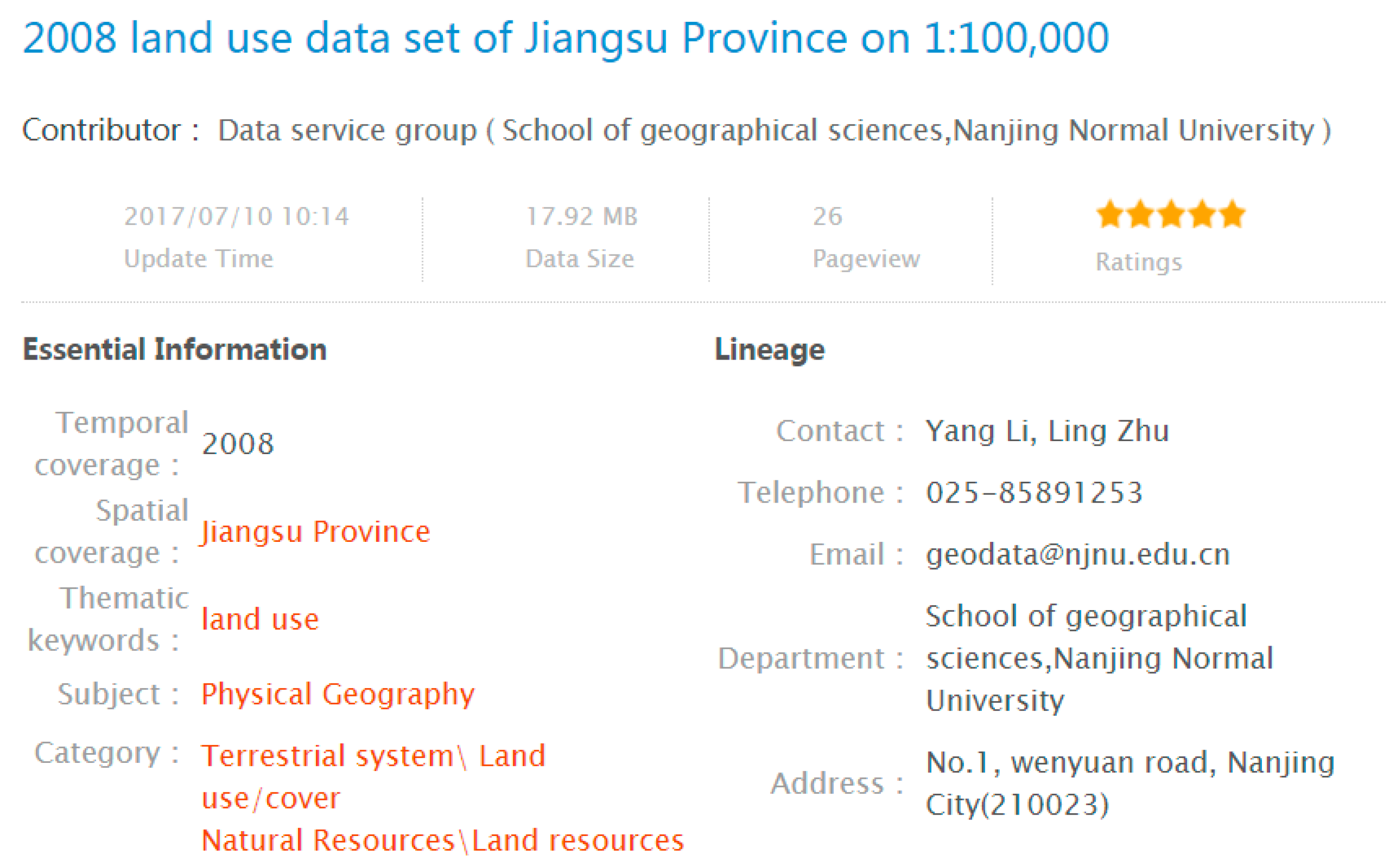
NESSDSI utilizes the ISO19115-based metadata to describe geospatial datasets [63]. Users search for the required data set via the metadata. The metadata of NESSDSI includes the data set title, data set language, a set of thematic keywords, abstract, category, spatial coverage, temporal coverage, format, lineage, and so on (The spatial coverage was represented by a geographic bounding box and a geographic description in NESSDSI. Parts of the metadata of a geospatial dataset in NESSDSI are shown in Figure 4). All the metadata and datasets can be openly accessed. We extracted 7169 geospatial data sets and their metadata from NESSDSI and applied TLRM to realize the semantic retrieval of geospatial data. Then, we compared the retrieval results between semantic retrieval and the traditional retrieval methods, which were mainly keyword-matching techniques.

In general, geographic information retrieval concerns the retrieval of thematically and geographically relevant information resources [64,65,66]. A GIR facility must evaluate the relatedness in terms of both the theme and spatial location (sometimes the temporal similarity is also evaluated, but it is not the most common situation). For geospatial data retrieval, it is required for users to type the search words of a theme and location. For example, when users are searching for the land use data set of San Francisco, they usually type a keyword pair (“land use”, “San Francisco”) to retrieve data in a geospatial data sharing website. Hence, we devise the following algorithm to retrieve geospatial data:

$$t=w_1\cdot x+w_2\cdot y$$

(16)

where $x$ is the thematic relatedness between the theme words the user typed and the thematic keywords of geospatial data, $y$ is the geographical relatedness between the locations the user typed and the spatial coverage of the geospatial data, and $t$ is the Matching Score (MS) between the data set that user desired and the geospatial data set from NESSDSI. In addition, $w_1$ and $w_2$ are weights in the interval $\in$ [0,1] and $w_1+w_2=1$ that can be determined by using the weight measurement method (WMM) of the analytic hierarchy process (AHP) (hereafter referred to as AHP-WMM) [67]. The detailed steps of AHP-WMM are as follows: First, we should establish a pairwise comparison matrix of the relative importance of all factors that affect the same upper-level goal. Then, domain experts establish pairwise comparison scores using a 1–9 preference scale. The normalized eigenvector of the pairwise comparison matrix is regarded as the weight of the factors. If the number of factors is more than two, a consistency check is required. The standard to pass the consistency check is that the consistency ratio (CR) is less than 0.1. The weights of $w_1$ and $w_2$ calculated by AHP-WMM are 0.667 and 0.333 respectively.

Recall is the ratio of the number of retrieved relevant records to the total number of relevant records in the database. Precision is the ratio of the number of retrieved relevant records to the total number of retrieved irrelevant and relevant records. We will compare the recall and precision between the traditional keyword-matching technique and the semantic retrieval technique based on the TLRM proposed in this article.

A traditional GIR search engine based on a keyword-matching technique will match the theme and location keywords typed by users with the thematic keywords and geospatial coverage description of geospatial metadata, respectively. If the two are both successfully matched, $x$ and $y$ are equal to 1, and MS is equal to 1. Otherwise, MS is equal to 0.

Our semantic retrieval techniques will not only match the user typed theme keywords with that of geospatial metadata, but also match the synonyms, hyponyms, hypernyms, and the synonyms of hyponyms and hypernyms of the typed theme keywords with that of geospatial metadata to search for geospatial data set within a larger range. At the same time, the relatedness between the typed theme keyword and its expansions is computed by using our TLRM which will be the value of $x$. For the sake of simplicity, we will also match location keywords with the geospatial coverage description of geospatial metadata. If the location keywords the user typed match the geospatial coverage description of geospatial metadata, then $y$ is equal to 1, otherwise, $y$ = 0. The retrieved data sets both have $x>0$ and $y>0$.

Based on the devised experiment above, we typed 30 pairs of the most frequently used keywords which were derived from the user access logs of NESSDSI to search for data in 7169 geospatial datasets. In 2017, the users of NESSDSI typed 60085 keywords. The 30 pairs of keywords were used 19,164 times. Then we computed the Recall and Precision of each pair of keywords for the traditional keyword-matching and our semantic retrieval techniques. The 30 pairs of keywords and their Recall and Precision are listed in

Table 5. The 30 pairs of keywords and the Recall and Precision for keyword-matching and semantic retrieval techniques.

ID	Theme	Location	Keyword Matching		Semantic Retrieval
			Recall	Precision	Recall	Precision
1	Basic geographic data	China	6/20	6/6	6/20	6/6
2	Land use	China	20/38	20/20	38/38	38/38
3	Population	China	19/161	19/19	19/161	19/19
4	Social economy	China	26/30	26/26	30/30	30/55
5	Landform	China	5/7	5/5	6/7	6/7
6	Soil	China	49/63	49/49	50/63	50/50
7	Desert	China	4/4	4/4	4/4	4/4
8	Lake	China	18/20	18/19	19/20	19/20
9	Natural resources	China	4/26	4/4	18/26	18/21
10	Wetland	China	5/6	5/5	5/6	5/5
11	Water environment	Taihu Lake	22/23	22/22	22/23	22/22
12	Administrative division	Shanghai	14/44	14/14	14/44	14/14
13	Remote sensing inversion	China	16/33	16/16	16/33	16/16
14	Meteorological observation	Tibet Plateau	8/9	8/8	9/9	9/9
15	Cyanobacterial bloom inversion	Taihu Lake	18/20	18/18	18/20	18/18
16	Precipitation	Tibet Plateau	20/26	20/20	26/26	26/33
17	Remote-sensing image	China	9/28	9/20	28/28	28/35
18	River	Yangtze River Basin	5/7	5/5	7/7	7/7
19	Hydro-meteorological data	Yangtze River	15/16	15/15	16/16	16/16
20	Aerosol	China	5/10	5/5	10/10	10/11
21	Biological resources	China	1/20	1/1	19/20	19/24
22	Land Cover	China	17/46	17/17	46/46	46/46
23	Climate	Tibet Plateau	10/39	10/10	32/39	32/32
24	Geomagnetism	Beijing Ming Tombs	19/19	19/19	19/19	19/19
25	Ecosystem	Tibet Plateau	13/66	13/17	13/66	13/17
26	Ecological environment	Xinjiang	8/54	8/9	16/54	16/17
27	Water quality	Taihu Lake	6/24	6/6	6/24	6/6
28	Air temperature	China	5/12	5/5	9/12	9/16
29	Natural disaster	China	5/8	5/5	7/8	7/7
30	Fish	China	12/13	12/12	12/13	12/12

.

Among the 30 queries in Table 5, the recall for 18 queries was improved by our semantic retrieval techniques, while it was unchanged for the other 12; the precision of 20 queries was unchanged, with 3 queries increased and 7 queries decreased. Our semantic retrieval techniques can improve the recall of geospatial data retrieval in most situations but decrease the precision in minority queries according to the evaluation results of the 30 most frequently used queries of NESSDSI. Moreover, our semantic retrieval techniques can rank the retrieval result. For example, the retrieval results of <‘Natural resources’, ‘China’> for the two retrieval methods are shown in

Table 6. Retrieval results of keywords matching method in 7169 data sets of NESSDSI.

ID	Data Set Title	MS
1	1988 the distribution data set of natural resources in china on 1:4000,000	1
2	1992 the distribution data set of natural resources in china on 1:4000,000	1
3	1993 the distribution data set of natural resources in china on 1:4000,000	1
4	1977 the distribution data set of natural resources in china on 1:4000,000	1

and

Table 7. Retrieval results of semantic retrieval techniques based on TLRM in 7169 data sets of NESSDSI.

ID	Data Set Title	MS
1	1988 the distribution data set of natural resources in china on 1:4000,000	1
2	1992 the distribution data set of natural resources in china on 1:4000,000	1
3	1993 the distribution data set of natural resources in china on 1:4000,000	1
4	1977 the distribution data set of natural resources in china on 1:4000,000	1
5	1997 forest and biological resources data set of china	0.84
6	2002 the third-level basin classification data set in china on 1:250,000	0.838
7	2002 the second-level basin classification data set in china on 1:250,000	0.838
8	2002 the primary-level basin classification data set in china on 1:250,000	0.838
9	2000 industrial water data set of China on 1 KM Grid	0.838
10	2000 total water consumption data set of China on 1 KM Grid	0.838
11	1986–2003 the energy resources data set of China	0.837
12	2003 the energy resources statistics data set of China	0.837
13	2004 the energy resources statistics data set of China	0.837
14	2005 the energy resources statistics data set of China	0.837
15	2006 the energy resources statistics data set of China	0.837
16	2007 the energy resources statistics data set of China	0.837
17	1980s data set of arable land suitable for farmland in china on 1:4,000,000	0.836
18	1980s quality of cultivated land data set in china on 1:4,000,000	0.836
19	1980s land resources data set in china on 1:1,000,000	0.836
20	China 1 KM classification of suitability land Grid Dataset (1980s)	0.836
21	1990s land resources data set in china on 1:1,000,000	0.836

.

It is obvious that semantic retrieval techniques based on TLRM are more capable of discovering geospatial data. The semantic retrieval techniques can find the data sets of subtypes of natural resources, such as the land resources, energy resources, water resources, and biological resources data sets in this example, though some of the data sets (ID: 6–8) are not the correct results. Furthermore, using the TLRM we can quantify the Matching Score between the query of users and the geospatial data. The retrieved geospatial data sets can be ranked by matching scores. With the ranked results users can find data of interest more quickly.

6. Discussion

6.1. Findings of Simulating Functions for Relatedness Computing

Human similarity/relatedness judgement is a type of nonlinear process. Finding accurate functions to simulate the process is extremely difficult. We can just intuitively and empirically derive the measures. For example, we know that exponential-decay functions are universal laws of stimulus generalization for psychological science [45]; thus we use the function $f_1(l)=e^{-\theta l}$ to represent the influence of semantic distance to relatedness. Is it accurate? No one is sure. We believe that our measure may be improved further if the true nonlinear function is found. One way to obtain the optimal nonlinear function may be to use an Artificial Neural Network to simulate the human judgement process. This deserves further research in the future.

6.2. Influence of Lexical Databases

Referring to the results in Table 4, we find that the correlations between values given by TLRM and GTRD in terms of different lexical databases are slightly different. The reason is that different lexical databases provide different similarity/relatedness for the top term pairs in the thesaurus.

Table 8. The top terms’ relatedness computed by different lexical database-based methods.

Terminology Pair	WordNet Relatedness [24]	HowNet Relatedness [28]
soil—frozen soil	0.8708	0.348
climate—landscape	0.4203	0.6186
city—industry	0.3164	0.120
climate—environment	0.2975	0.7222
environment—landscape	0.2914	0.619
climate—soil	0.265	0.4444
climate—weather	0.2532	1.000
environment—soil	0.2146	0.0444
environment—weather	0.1686	0.0444
climate—city	0.1463	0.2087
climate—industry	0.1042	0.11628
climate—transportation	0.0933	0.211

lists the relatedness of the top terms of the terminologies in GTRD computed by WordNet and HowNet-based measures [24,28], respectively.

“Climate”, “weather”, “environment”, “landscape”, “soil”, “frozen soil”, “city”, “industry”, “transportation” are the top terms of nine term trees in the thesaurus. Relatedness values of these terminology pairs computed by different generic lexical database based methods are consistent with human intuition in different degrees. The relatedness computed by WordNet seems to be slightly better than that computed by HowNet on the whole, although they are all not accurate. The precision of relatedness computed by the generic lexical database-based method has an influence on the precision of TLRM.

7. Conclusions

In this article, we described the thesaurus–lexical relatedness measure (TLRM), a measure to capture the relatedness of any two terms in the Thesaurus for Geographic Science. We successfully interlinked the term trees in the thesaurus and quantified the relations of terms. We built a new evaluative baseline for geo-terminology-semantic relatedness and the cognitive plausibility of the TLRM was evaluated, obtaining high correlations with expert judgements. Finally, we applied the TLRM to geospatial data retrieval and improved the recall of geospatial data retrieval to some extent according to the evaluation results of 30 most frequently used queries of the NESSDSI.

We first combined the generic lexical database with a professional controlled vocabulary and proposed new algorithms to compute the relatedness of any two terms in the thesaurus. Our algorithms are not only suitable for geography, but also for other disciplines as well.

Although the TLRM obtained a high cognitive plausibility, some limitations remain to be addressed in future research. Despite the fact that there are more than 10,000 terminologies in the thesaurus, we cannot guarantee that all geographic terminologies have been included. Automatically and continually adding unrecorded geographic terminologies to the thesaurus database remains a challenge to be addressed. Furthermore, there are only three types of relationships between terminologies in a thesaurus. This is both an advantage and a disadvantage. The advantage is that it is relatively easy to build a thesaurus covering most of the terminologies in a discipline. The disadvantage is that three kinds of relationships are not sufficient to precisely represent the relationships between geographic terminologies. Geo-knowledge triples may be alternatives in the future. In addition, we evaluated the TLRM on its ability to simulate expert judgements on the entire range of semantic relatedness, that is from very related to very unrelated concepts. Given that no cognitive plausibility evaluation is fully generalizable, robust evidence can only be constructed by cross-checking different evaluations. For example, complementary indirect evaluations could focus on specific relatedness-based tasks, such as word sense disambiguation.

In the next study, we will share and open the thesaurus database to the public and any geography expert can add terms to or revise the database. We will render it a consensual geographic knowledge graph built via expert crowdsourcing. At the same time, we will continue to find the optimal functions to further improve the cognitive plausibility of TLRM and cross-check different evaluations. We are planning to build a geography semantic sharing network and share the relatedness measure interface with all users.

References

- Rada, R.; Mili, H.; Bicknell, E.; Blettner, M. Development and application of a metric on semantic nets. IEEE Trans. Syst. Man Cybern. 1989, 19, 17–30. [Google Scholar] [CrossRef]
- Ballatore, A.; Bertolotto, M.; Wilson, D.C. An evaluative baseline for geo-semantic relatedness and similarity. Geoinformatica 2014, 18, 747–767. [Google Scholar] [CrossRef]
- Ballatore, A.; Wilson, D.C.; Bertolotto, M. Computing the semantic similarity of geographic terms using volunteered lexical definitions. Int. J. Geogr. Inf. Sci. 2013, 27, 2099–2118. [Google Scholar] [CrossRef]
- Rissland, E.L. Ai and similarity. IEEE Intell. Syst. 2006, 21, 39–49. [Google Scholar] [CrossRef]
- Harispe, S.; Ranwez, S.; Janaqi, S.; Montmain, J. Semantic Similarity from Natural Language and Ontology Analysis; Morgan & Claypool: Nımes, France, 2015; pp. 2–7. [Google Scholar]
- Li, Y.; Bandar, Z.A.; McLean, D. An approach for measuring semantic similarity between words using multiple information sources. IEEE Trans. Knowl. Data Eng. 2003, 15, 871–881. [Google Scholar]
- Rodríguez, M.A.; Egenhofer, M.J. Comparing geospatial entity classes: An asymmetric and context-dependent similarity measure. Int. J. Geogr. Inf. Sci. 2004, 18, 229–256. [Google Scholar] [CrossRef]
- Purves, R.S.; Jones, C.B. Geographic Information Retrieva; Sigspatial Special: New York, NY, USA, 2011; pp. 2–4. [Google Scholar]
- Zhu, Y.; Zhu, A.-X.; Song, J.; Zhao, H. Multidimensional and quantitative interlinking approach for linked geospatial data. Int. J. Digit. Earth 2017, 10, 1–21. [Google Scholar] [CrossRef]
- Ballatore, A.; Bertolotto, M.; Wilson, D.C. A structural-lexical measure of semantic similarity for geo-knowledge graphs. ISPRS Int. J. Geo-Inf. 2015, 4, 471–492. [Google Scholar] [CrossRef]
- Krzysztof, J.; Keßler, C.; Mirco, S.; Marc, W.; Ilija, P.; Martin, E.; Boris, B. Algorithm, implementation and application of the sim-dl similarity server. In Proceedings of the International Conference on Geospatial Semantics, Mexico City, Mexico, 29–30 November 2007; Volume 4853, pp. 128–145. [Google Scholar]
- International Organization for Standardization (ISO). Information and Documentation-Thesauri and Interoperability with Other Vocabularies—Part 1: Thesauri for Information Retrieval (International Standard No. ISO 25964-1); ISO-25964-1; International Organization for Standardization: Geneva, Switzerland, 2011. [Google Scholar]
- Kless, D.; Milton, S.K.; Kazmierczak, E.; Lindenthal, J. Thesaurus and ontology structure: Formal and pragmatic differences and similarities. J. Assoc. Inf. Sci. Technol. 2014, 66, 1348–1366. [Google Scholar] [CrossRef]
- Kless, D.; Milton, S.K.; Kazmierczak, E. Relationships and relata in ontologies and thesauri: Differences and similarities. Appl. Ontol. 2012, 7, 401–428. [Google Scholar]
- Riekert, W.-F. Automated retrieval of information in the internet by using thesauri and gazetteers as knowledge sources. J. Univ. Comput. Sci. 2002, 8, 581–590. [Google Scholar]
- Guo, Y.; An, F.T.; Liu, Z.T.; Sun, Y.H.; Yang, Y.F.; Cai, G.B.; Ding, H.Y.; Wen, C.S.; Zhang, Y.H.; Zhang, Y.B.; et al. Thesaurus for Geographic Sciences; Science Press: Beijing, China, 1995; pp. 1–615. [Google Scholar]
- Miller, G.A. Wordnet: A lexical database for english. Commun. ACM 1995, 38, 39–41. [Google Scholar] [CrossRef]
- About Wordnet. Available online: http://wordnet.princeton.edu (accessed on 20 December 2017).
- Resnik, P. Using information content to evaluate semantic similarity in a taxonomy. In Proceedings of the 14th International Joint Conference on Artificial Intelligence, Montreal, QC, Canada, 20–25 August 1995; pp. 448–453. [Google Scholar]
- Jiang, J.J.; Conrath, D.W. Semantic similarity based on corpus statistics and lexical taxonomy. In Proceedings of the International Conference Research on Computational Linguistics, Taipei, Taiwan, 22–24 August 1997. [Google Scholar]
- Lin, D. An information-theoretic definition of similarity. In Proceedings of the Fifteenth International Conference on Machine Learning, San Francisco, CA, USA, 24–27 July 1998; pp. 296–304. [Google Scholar]
- Leacock, C.; Chodorow, M. Combining local context and wordnet similarity for word sense identification. In WordNet: An Electronic Lexical Database; MIT Press: Cambridge, MA, USA, 1998; pp. 265–283. [Google Scholar]
- Wu, Z.; Palmer, M.S. Verbs semantics and lexical selection. In Proceedings of the 32nd Annual Meeting on Association for Computational Linguistics, Las Cruces, NM, USA, 27–30 June 1994; pp. 133–138. [Google Scholar]
- Patwardhan, S.; Pedersen, T. Using wordnet-based context vectors to estimate the semantic relatedness of concepts. In Proceedings of the Eacl Workshop on Making Sense of Sense: Bringing Computational Linguistics and Psycholinguistics Together, Trento, Italy, 3–7 April 2006. [Google Scholar]
- Ballatore, A.; Bertolotto, M.; Wilson, D.C. The semantic similarity ensemble. J. Spat. Inf. Sci. 2013, 27–44. [Google Scholar] [CrossRef]
- Hownet Knowledge Database. Available online: http://www.keenage.com/ (accessed on 10 December 2017).
- Li, H.; Zhou, C.; Jiang, M.; Cai, K. A hybrid approach for chinese word similarity computing based on hownet. In Proceedings of the Automatic Control and Artificial Intelligence, Xiamen, China, 3–5 March 2012; pp. 80–83. [Google Scholar]
- Liu, Q.; Li, S. Word similarity computing based on hownet. Comput. Linguist. Chin. Lang. Process. 2002, 7, 59–76. [Google Scholar]
- Introduction to HowNet. Available online: http://www.keenage.com/zhiwang/e_zhiwang.html (accessed on 25 December 2017).
- Landauer, T.K.; McNamara, D.S.; Deniss, S.; Kintsch, W. Handbook of Latent Semantic Analysis; Lawrence Erlbaum Associates: Mahwah, NJ, USA, 2007. [Google Scholar]
- Turney, P.D. Mining the web for synonyms: Pmi-ir versus lsa on toefl. In Proceedings of the 12th European Conference on Machine Learning, Freiburg, Germany, 5–7 September 2001; pp. 491–502. [Google Scholar]
- Mihalcea, R.; Corley, C.; Strapparava, C. Corpus-based and knowledge-based measures of text semantic similarity. In Proceedings of the 21st National Conference on Artificial Intelligence, Boston, MA, USA, 16–20 July 2006; pp. 775–780. [Google Scholar]
- Qiu, H.; Yu, W. Conceptual similarity measurement of term based on domain thesaurus. In Proceedings of the Seventh International Conference on Machine Learning and Cybernetics, Kunming, China, 12–15 July 2008; pp. 2519–2523. [Google Scholar]
- McMath, C.F.; Tamaru, R.S.; Rada, R. A graphical thesaurus-based information retrieval system. Int. J. Man-Mach. Stud. 1989, 31, 121–147. [Google Scholar] [CrossRef]
- Rada, R.; Barlow, J.; Potharst, J.; Zanstra, P.; Bijstra, D. Document ranking using an enriched thesaurus. J. Doc. 1991, 47, 240–253. [Google Scholar] [CrossRef]
- Golitsyna, O.L.; Maksimov, N.V.; Fedorova, V.A. On determining semantic similarity based on relationships of a combined thesaurus. Autom. Doc. Math. Linguist. 2016, 50, 139–153. [Google Scholar] [CrossRef]
- Qichen, H.; Dongmei, L. Semantic model with thesaurus for forestry information retrieval. J. Front. Comput. Sci. China 2016, 10, 122–129. [Google Scholar]
- Cerba, O.; Jedlicka, K. Linked forests: Semantic similarity of geographical concepts “forest”. Open Geosci. 2016, 8, 556–566. [Google Scholar]
- Tversky, A. Features of similarity. Psychol. Rev. 1977, 84, 327–352. [Google Scholar] [CrossRef]
- Schwering, A.; Martin, R. Spatial relations for semantic similarity measurement. In Proceedings of the International Conference on Perspectives in Conceptual Modeling, Klagenfurt, Austria, 24–28 October 2005; pp. 259–269. [Google Scholar]
- Cruz, I.F.; Sunna, W. Structural alignment methods with applications to geospatial ontologies. Trans. GIS 2008, 12, 683–711. [Google Scholar] [CrossRef]
- Ballatore, A.; Bertolotto, M.; Wilson, D.C. Geographic knowledge extraction and semantic similarity in openstreetmap. Knowl. Inf. Syst. 2013, 37, 61–81. [Google Scholar] [CrossRef]
- Ballatore, A.; Wilson, D.C.; Bertolotto, M. A holistic semantic similarity measure for viewports in interactive maps. In Proceedings of the Web andWireless Geographical Information Systems 11th International Symposium, Naples, Italy, 12–13 April 2012; pp. 151–166. [Google Scholar]
- Index Term. Available online: https://en.wikipedia.org/wiki/Index_term (accessed on 25 December 2017).
- Shepard, R.N. Toward a universal law of generalization for psychological science. Science 1987, 237, 1317–1323. [Google Scholar] [CrossRef] [PubMed]
- Liu, H.-Z.; Bao, H. Concept vector for similarity measurement based on hierarchical domain structure. Comput. Inform. 2011, 30, 881–900. [Google Scholar]
- Corley, C.; Mihalcea, R. Measuring the semantic similarity of texts. In Proceedings of the ACL Workshop on Empirical Modeling of Semantic Equivalence and Entailment, Ann Arbor, MI, USA, 30 June 2005; pp. 13–18. [Google Scholar]
- Miller, G.A.; Charles, W.G. Contextual correlates of semantic similarity. Lang. Cogn. Neurosci. 1991, 6, 1–28. [Google Scholar] [CrossRef]
- Rubenstein, H.; Goodenough, J. Contextual correlates of synonymy. Commun. ACM 1965, 8, 627–633. [Google Scholar] [CrossRef]
- Finkelstein, L.; Gabrilovich, E.; Matias, Y.; Rivlin, E.; Solan, Z.; Wolfman, G.; Ruppin, E. Placing search in context: The concept revisited. ACM Trans. Inf. Syst. 2002, 20, 116–131. [Google Scholar] [CrossRef]
- Nelson, D.L.; Dyrdal, G.M.; Goodmon, L.B. What is preexisting strength? Predicting free association probabilities, similarity ratings, and cued recall probabilities. Psychon. Bull. Rev. 2005, 12, 711–719. [Google Scholar] [CrossRef] [PubMed]
- Stigler, S.M. Francis galton’s account of the invention of correlation. Stat. Sci. 1989, 4, 73–79. [Google Scholar] [CrossRef]
- Lebreton, J.; Burgess, J.R.D.; Kaiser, R.B.; Atchley, E.K.P.; James, L.R. The restriction of variance hypothesis and interrater reliability and agreement: Are ratings from multiple sources really dissimilar? Organ. Res. Methods 2003, 6, 80–128. [Google Scholar] [CrossRef]
- James, L.R.; Demaree, R.G.; Wolf, G. An assessment of within-group interrater agreement. J. Appl. Psychol. 1993, 78, 306–309. [Google Scholar] [CrossRef]
- Lebreton, J.; Senter, J.L. Answers to 20 questions about interrater reliability and interrater agreement. Organ. Res. Methods 2008, 11, 815–852. [Google Scholar] [CrossRef]
- Rodgers, J.; Nicewander, A. Thirteen ways to look at the correlation coefficient. Am. Stat. 1988, 42, 59–66. [Google Scholar] [CrossRef]
- Kruskal, W.H. Ordinal measures of association. J. Am. Stat. Assoc. 1958, 53, 814–861. [Google Scholar] [CrossRef]
- Kendall, M.G.; Smith, B.B. The problem of m rankings. Ann. Math. Stat. 1939, 10, 275–287. [Google Scholar] [CrossRef]
- James, L.R.; Demaree, R.G.; Wolf, G. Estimating within-group interrater reliability with and without response bias. J. Appl. Psychol. 1984, 69, 85–98. [Google Scholar] [CrossRef]
- Levenberg, K.A. A method for the solution of vertain problems in least squares. Q. Appl. Math. 1944, 2, 164–168. [Google Scholar] [CrossRef]
- Marquardt, D.W. An algorithm for least-squares estimation of nonlinear parameter. J. Soc. Ind. Appl. Math. 1963, 11, 431–441. [Google Scholar] [CrossRef]
- Powell, M.J.D. A Fortran Subroutine for Solving Systems of Non-Linear Algebraic Equations; Atomic Energy Research Establishment: London, UK, 1968; pp. 115–161. [Google Scholar]
- ISO. Geographic Information—Metadata; ISO-19115; ISO: Geneva, Switzerland, 2003. [Google Scholar]
- Frontiera, P.; Larson, R.R.; Radke, J. A comparison of geometric approaches to assessing spatial similarity for gir. Int. J. Geogr. Inf. Sci. 2008, 22, 337–360. [Google Scholar] [CrossRef]
- Bordogna, G.; Ghisalberti, G.; Psaila, G. Geographic information retrieval: Modeling uncertainty of user’s context. Fuzzy Sets Syst. 2012, 196, 105–124. [Google Scholar] [CrossRef]
- Aissi, S.; Gouider, M.S.; Sboui, T.; Said, L.B. Enhancing spatial data warehouse exploitation: A solap recommendation approach. In Proceedings of the 17th IEEE/ACIS International Conference on Software Engineering, Artificial Intelligence, Networking and Parallel/Distributed Computing (SNPD), Shanghai, China, 30 May–1 June 2016; pp. 457–464. [Google Scholar]
- Saaty, T.L. How to make a decision: The analytic hierarchy process. Eur. J. Oper. Res. 1990, 48, 9–26. [Google Scholar] [CrossRef]
Figure 1.
Two term trees from Thesaurus for Geographic Science.
Figure 2.
Word description of HowNet.
Figure 3.
Hierarchy of fishing pole DEF.
Figure 4.
Parts of the metadata of a geospatial dataset in National Earth System Science Data Sharing Infrastructure (NESSDSI).