High-Performance Geospatial Big Data Processing System Based on MapReduce

IoT Research Division, Electronics and Telecommunications Research Institute (ETRI), 218 Gajeong-ro, Yuseong-gu, Daejeon 34129, Korea
*
Author to whom correspondence should be addressed.
ISPRS Int. J. Geo-Inf. 2018, 7(10), 399; https://doi.org/10.3390/ijgi7100399
Submission received: 21 August 2018
/
Revised: 30 September 2018
/
Accepted: 4 October 2018
/
Published: 6 October 2018
(This article belongs to the Special Issue Distributed and Parallel Architectures for Spatial Data)
Abstract
:With the rapid development of Internet of Things (IoT) technologies, the increasing volume and diversity of sources of geospatial big data have created challenges in storing, managing, and processing data. In addition to the general characteristics of big data, the unique properties of spatial data make the handling of geospatial big data even more complicated. To facilitate users implementing geospatial big data applications in a MapReduce framework, several big data processing systems have extended the original Hadoop to support spatial properties. Most of those platforms, however, have included spatial functionalities by embedding them as a form of plug-in. Although offering a convenient way to add new features to an existing system, the plug-in has several limitations. In particular, while executing spatial and nonspatial operations by alternating between the existing system and the plug-in, additional read and write overheads have to be added to the workflow, significantly reducing performance efficiency. To address this issue, we have developed Marmot, a high-performance, geospatial big data processing system based on MapReduce. Marmot extends Hadoop at a low level to support seamless integration between spatial and nonspatial operations of a solid framework, allowing improved performance of geoprocessing workflow. This paper explains the overall architecture and data model of Marmot as well as the main algorithm for automatic construction of MapReduce jobs from a given spatial analysis task. To illustrate how Marmot transforms a sequence of operators for spatial analysis to map and reduce functions in a way to achieve better performance, this paper presents an example of spatial analysis retrieving the number of subway stations per city in Korea. This paper also experimentally demonstrates that Marmot generally outperforms SpatialHadoop, one of the top plug-in based spatial big data frameworks, particularly in dealing with complex and time-intensive queries involving spatial index.
1. Introduction
In the environment of the Internet of Things (IoT), various sensors have been mounted on objects in diverse domains, generating huge volumes of data at high speed [1,2]. A significant portion of sensor big data is geospatial data describing objects in relation to geographic information [3,4]. In general, geospatial big data refers to geographic data sets that cannot be processed using standard computing systems [3,4,5].
The general consensus among researchers from various domains is that “80% of data is geographic” [3,6,7,8,9]. The United Nations Initiative on Global Geospatial Information Management (UN-GGIM) reported that 2.5 quintillion bytes of data is created every day and a significant portion includes location components [10]. Google generates approximately 25 PB of data daily, a large portion of which consists of spatiotemporal characteristics [11]. The McKinsey Global Institute estimates the portion of spatial aspect data was about 1 PB in 2009 and is growing at an annual rate of 20% [12]. Due to the exponential growth of geospatial big data, utilization of data has become a global interest, increasingly drawing the attention not only of industry and academia, but also government agencies.
To promote openness and availability of geospatial big data, the US Federal Geographic Data Committee (FGDC) has defined the concept of National Spatial Data Infrastructure (NSDI) and preserves place-based data at all levels of government, private and nonprofit sectors, and academia. The FGDC provides rich sets of geospatial data to the public to support business, government agencies, or their partners. Geospatial One-Stop (GOS) is an initiative consistent with the goals of NSDI. It establishes a web-based portal (www.geodata.gov) for one-stop access to geospatial data and services and opens a developed portal to federal, state, and local governments, along with private citizens [13]. The EU directive, INSPIRE (Infrastructure for Spatial Information in Europe) project, plays an equivalent role for GOS [14,15]. It aims to benefit all levels of public authorities in Europe by producing and sharing integrated and quality geospatial information of EU Member States. In Oceania and Asia, there are also similar initiatives such as the Australian SDI [16] and Indian SDI [17], respectively.
The increasing volume and diverse sources (e.g., smart phones) of collected geospatial big data have created challenges in storing, managing, and processing data. In addition to the general characteristics of big data, the unique properties of spatial data such as computationally intensive processing of the time component make dealing with geospatial big data even more complicated. To some degree, traditional distributed and parallel processing frameworks make it possible to meet performance requirements for handling large-scale data. It has been several years since developers implemented an SQL-based system and operated it in a parallel way, though it was inadequate to deal efficiently with large volumes of data. System architecture has steadily evolved and a parallel database was designed to allow multiple data instances to share a single database with improvement in performance in parallel computing environments [18]. This is an efficient approach providing speedup and scale up for massive data, compared to traditional SQL systems.
Recently, several big data platforms have been built to facilitate developers of big data applications on a distributed and parallel computing platform. Particularly, Apache Hadoop [19] has existed for years and proven to be a mature and very popular platform for big data analysis for various applications. Hadoop is an open source MapReduce implementation being used at major corporations such as IBM, Amazon, Facebook, and Yahoo. Hadoop, however, is ill-equipped to support geospatial big data because its core structure does not consider the unique properties of spatial data (e.g., spatial data types). Also, the efficiency of operations (e.g., spatial queries) is limited on those platforms since the Hadoop‘s internal system is uninformed about spatial data.
To take advantage of the Hadoop/MapReduce environment in dealing with geospatial big data, several systems supporting spatial properties on Hadoop have emerged. ESRI has released a collection of GIS tools for spatial analysis [20] that provides access to the Hadoop system from ArcGIS products. In academia, Hadoop-GIS [21] is designed to support multiple types of spatial queries on MapReduce via skew-aware spatial partitioning to first partition spatial objects and then process them in parallel. Similarly, GPHadoop [22], a geoprocessing-enabled Hadoop platform, has been introduced to enable scalable geoprocessing to resolve geospatial related problems based on Hadoop and ESRI GIS tools. A main limitation of those Hadoop-based spatial systems is that they regard Hadoop as a black box and are therefore restricted by the limitations of the original Hadoop. To circumvent that issue, SpatialHadoop [23,24] has been designed, which injects spatial data awareness inside Hadoop making it more efficient to work with spatial data. SpatialHadoop, however, still presents a lack of integration with the core structure of Hadoop. For example, SpatialHadoop adds spatial data types or functions to the original Hadoop system as a form of plug-ins. However, compared to a solid framework, the performance of a plug-in based framework is limited by lacking seamless integration between spatial and nonspatial operations.
In this paper, we introduce the Marmot system, a Hadoop-based, high-performance data storage management system. It enables application developers having little working knowledge of big data technologies to implement high performance analysis tasks on geospatial big data. Compared with existing Hadoop-based spatial systems, the distinctive characteristics of Marmot can be summarized as follows.
- Marmot extends Hadoop at a low level and is a stream-based system supporting seamless integration between spatial and nonspatial operations in a solid framework.
- Marmot supports automatic construction of MapReduce jobs from a given spatial analysis task in ways to improve performance.
- Marmot allows developers to create various spatial applications by simply combining built-in spatial or nonspatial operators.
The rest of the paper is organized as follows. Section 2 shows our related work and Section 3 describes a systematic overview of Marmot including integration between spatial and nonspatial operations. Section 4 shows Marmot’s data model and Section 5 presents the main algorithm which maps a sequence of operators for spatial analysis to MapReduce jobs and discusses implementation of Marmot. An example of a spatial application using Marmot and its performance evaluation is described in Section 6 and Section 7, respectively. Finally, the discussion and conclusion along with our future work are presented in Section 8 and Section 9.
2. Related Work
Several platforms have been developed for the processing of big data. MapReduce [25] is a distributed and parallel programming framework and is very popular due to its simplicity, scalability, and fault-tolerance. There are two phases in the MapReduce model: Map phase and Reduce phases. The Map phase is used to receive data and generate intermediate key and value pairs; the Reduce phase is used to accept the intermediate results and combine them into a single result. Hadoop [19] is an implementation of MapReduce as an open source form, which has been widely adopted in a majority companies as their technology stack.
Although Hadoop is known as the most representative distributed processing framework for handling big data, it cannot be used for real-time processing because the data are batched to each node for a given job. Spark [26] is an in-memory based high performance distributed data analysis system designed to address Hadoop’s limitations. Unlike Hadoop, which is based on a batch processing engine, Spark can process data faster due to its in-memory computation policy. Although this feature provides advantages of low latency computation, there are also drawbacks such as requiring significantly more resources than Hadoop.
Most big data platforms, including Hadoop and Spark, have been designed without any specific consideration of spatial properties. A few platforms provide spatial functionalities [20,21,22,23,24], but they generally lack spatial properties and do not support advanced geospatial operations such as geospatial joins and geostatistical operations, which are imperative for advanced geospatial analytics. SpatialHadoop [22,23] has been developed to enable spatial operations by extending Hadoop layers: language, storage, MapReduce, and operations. Although SpatialHadoop has been known to overcome the limitations of existing spatial big data platforms and perform better than traditional Hadoop, it is still not sufficient in supporting in-depth geospatial analysis.
3. Marmot Overview
3.1. A Functional Architecture of High Performance
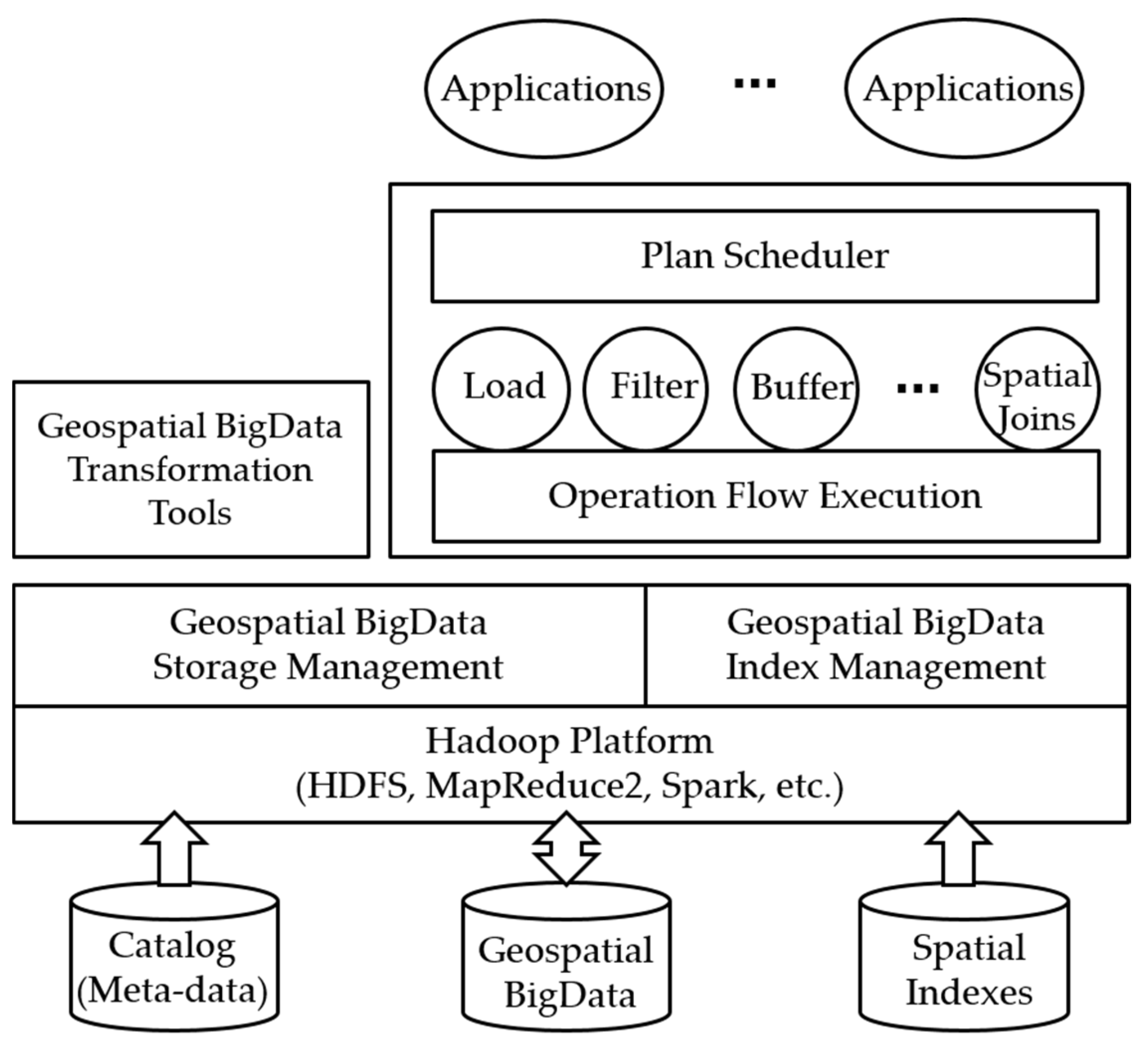
Marmot is a functional architecture that processes geospatial big data in parallel with MapReduce jobs for both batch and streaming services. A MapReduce job usually divides big data sets into separate chunks which are processed by map tasks in parallel. The framework sorts the results of the maps which are later input to reduce tasks.
Although MapReduce has been a highly popular framework for conducting parallelized distributed computing jobs, it is still not easy for developers to build complex geospatial big data applications. In fact, users of MapReduce often have analysis tasks which are too complicated to be transformed to MapReduce jobs. Such spatial tasks require handling the chain of multiple MapReduce steps where the output path of the data from previous MapReduce jobs becomes the input path to the next MapReduce job. To address this issue, Marmot supports automatic construction of one or more MapReduce tasks by taking on a spatial analysis task. When the task is transformed to MapReduce jobs, Marmot automatically controls the number of MapReduce jobs in a way to achieve better performance by decreasing the overhead of mapping and reducing.
Figure 1 shows a brief structure of Marmot which is based on a Hadoop framework. The core of Marmot consists of four main components: a plan scheduler, operation flow execution, geospatial big data storage management, and index management. This paper focuses on explaining how Marmot transforms a sequence of operators for spatial analysis to map and reduce functions. Specific content about other components is beyond the scope of this paper.
3.2. Integrating Spatial and Nonspatial Operations
NoSQL systems are very well-adapted to the environment offering high-performance information processing on a massive scale and so are increasingly used to deal with heavy demands of big data applications. Various NoSQL systems are currently available; however, only few provide spatial functionalities. MongoDB supports spatial indexing which allows users to execute spatial queries on a collection involving shapes and points, but it does not support many advanced geospatial operations which are essential for advanced geospatial analytics. PostGIS has more comprehensive geospatial functionalities but still provides only limited number of spatial data types and very few functions to handle them [27,28]. Thus, existing NoSQL systems needing to newly include or extend spatial functions generally use a form of plug-ins to support the extra feature within their systems. For example, Cassandra is extended to enable spatial data retrieval by extending its query language capabilities [28,29], and HBase is extended to support spatial indexes of Quad tree and K-d tree to enable range/kNN queries and point datasets [30].
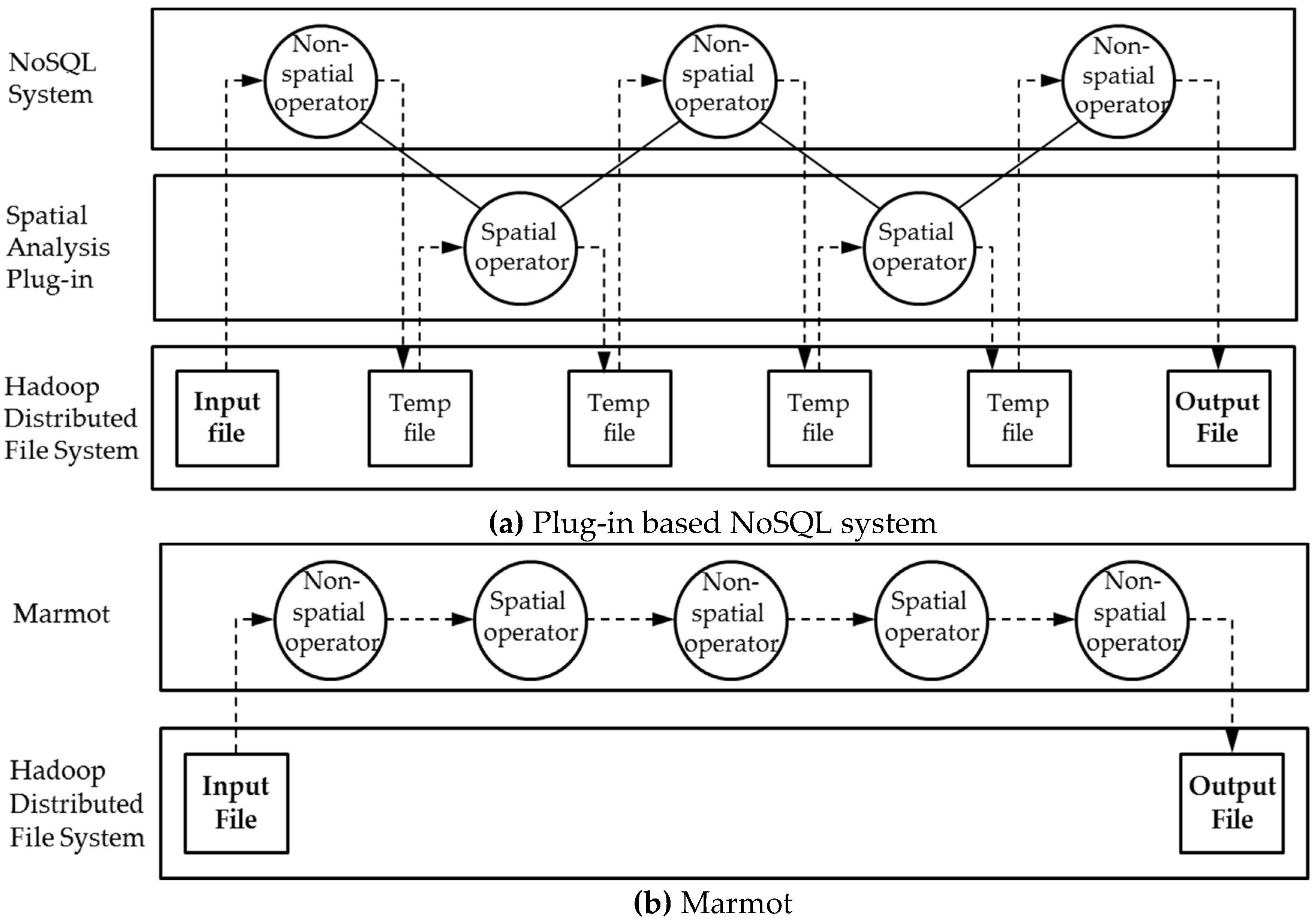
Though the plug-in offers a convenient way to add new features to an existing system, it carries several limitations as described in Figure 2a. First, it is inadequate to support seamless interactions between spatial and nonspatial operations. A NoSQL system basically treats plug-ins as legacy and generates temporary files while executing spatial and nonspatial operations by turns, obstructing improvements in workflow. Second, its performance is limited due to the high number of input/output operations while reading or writing temporary files. Furthermore, this input/output overhead increases with increases in file size, as well as the number of operations. From this, we assume that if we reduce the data transfer overhead between NoSQL and spatial plugins, we could improve data processing performance.
Marmot supports seamless interactions between spatial and nonspatial operations within a solid framework, as shown in Figure 2b. This is possible because Marmot is designed and developed by considering the data model and operations for processing spatial information from the initial phase of the development process. Most NoSQL systems, however, are designed with no consideration of spatial functionalities. This leads them to adopt plug-in based architecture when they want to embed spatial functionalities later on. Because both spatial and nonspatial operations are managed by one system, it is feasible to improve workflow. In addition, since temporary files do not need to be generated, the input/output overhead also decreases considerably regardless of file size or the number of operations for analysis.
4. Marmot Data Model
The term data model refers to an abstract model that arranges the structure of data and regulates their association with each other. Figure 3 shows the data model used in Marmot that corresponds mostly with the model in a standard relational database management system (RDBMS).
In Marmot, a Record corresponds to a record in RDBMS, the smallest unit of a data element consisting of one or more column values within a table. The definition of a Record in Marmot is shown in Definition 1.
| Definition 1. Record |
| public interface Record { |
| public RecordSchema getSchema(); |
| public Object get(String colName); |
| public Object get(int idx); |
| public Object[[] getAll(); |
| public void set(String colName, Object value); |
| public void set(int idx, Object value); |
| public void set(Record rec, Boolean removeOverflow); |
| public Geometry getGeometry(……); |
| public String getString(……); |
| } |
A RecordSet is a set of records corresponding to a table in RDBMS which provides forward-only access to a data source. A RecordSchema represents metadata consisting of information containing the names and types of columns composing a Record. All the Records included in a specific RecordSet are compliant with the same RecordSchema. The definitions of RecordSet and RecordSchema are shown in Definition 2 and Definition 3, respectively.
| Definition 2. RecordSet |
| public interface RecordSet { |
| RecordSchema getRecordSchema(); |
| Boolean next(Record record); |
| Record nextCopy(); |
| void close(); |
| Stream<Record> stream(); |
| List<Record> toList(); |
| Iterator<Record> iterator(); |
| } |
| Definition 3. RecordSchema |
| public class RecordSchema { |
| public int getColumnCount(); |
| public Boolean existsColumn(String colName); |
| public Column getColumn(String colName); |
| public Column getColumnAt(int idx); |
| public Collection<Column> getColumnAll(); |
| } |
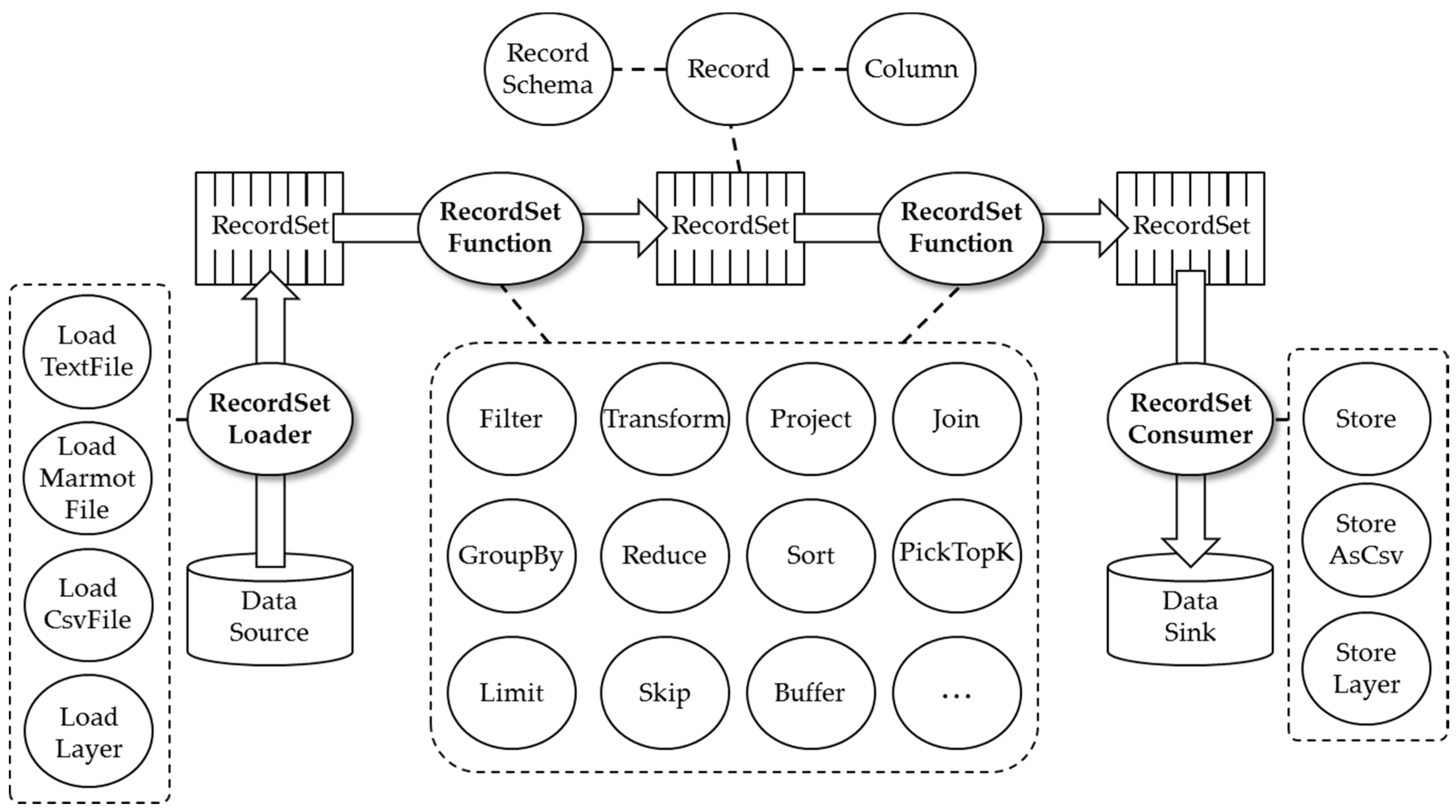
A RecordSetOperator is a processing unit using a RecordSet which corresponds to the concept of a relational operator in RDBMS. As the input and output of relational operators in RDBMS are a table, the input and output of a RecordSetOperator is a RecordSet. In Marmot, there are three types of a RecordSetOperator, as shown in Figure 4.
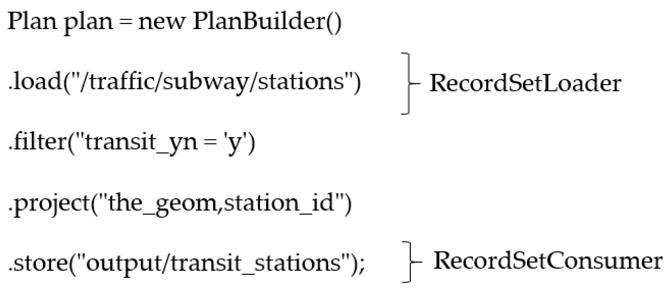
A RecordSetLoader is an operator that loads input data from outside data sources and converts it to RecordSet to be handled within Marmot. For example, loadTextFile reads a text file from a given path and converts it to a RecordSet. A RecordSetConsumer stores a RecordSet created within Marmot as the final result of a given analysis to a specified outside path. A Marmot code describing RecordSetLoader and RecordSetConsumer is given in Figure 5.
Lastly, the RecordSetFunction is an operator that takes a RecordSet as input data and outputs a new RecordSet. In Marmot, there are two types of a RecordSetFuntion: spatial operators and nonspatial operators. Spatial operators are functions taking input spatial data, analyzing various types of spatial relationships, and producing output spatial data. For example, Buffer is a spatial operator creating a new RecordSet which is the result of encompassing the area around a specific location based on a predefined distance. Project and Filter are examples of nonspatial operators, where Project produces a RecordSet composed only of specified columns; Filter generates a RecordSet consisting only of columns satisfying certain conditions.
The spatial and nonspatial operators currently supported in Marmot are shown in Table 1. Examples of their interfaces and usages are shown in Examples 1 and 2.
| Example 1. Nonspatial operators in RecordSetFuntion |
|
| Example 2. Spatial operators in RecordSetFuntion |
| • loadSpatialIndexJoin(condition, layer1, layer2, result_column1, result_colume2)[Usage] loadSpatialIndexJoin(SpatialPredicate.INTERSECTS, “admin/cadastral/clusters”, “admin/urban_area/clusters”, “*”, “*-{the_geom},the_geom as the_geom2”) |
5. Spatial Analysis using Marmot
5.1. Plan: A Chain of RecordSetOperators
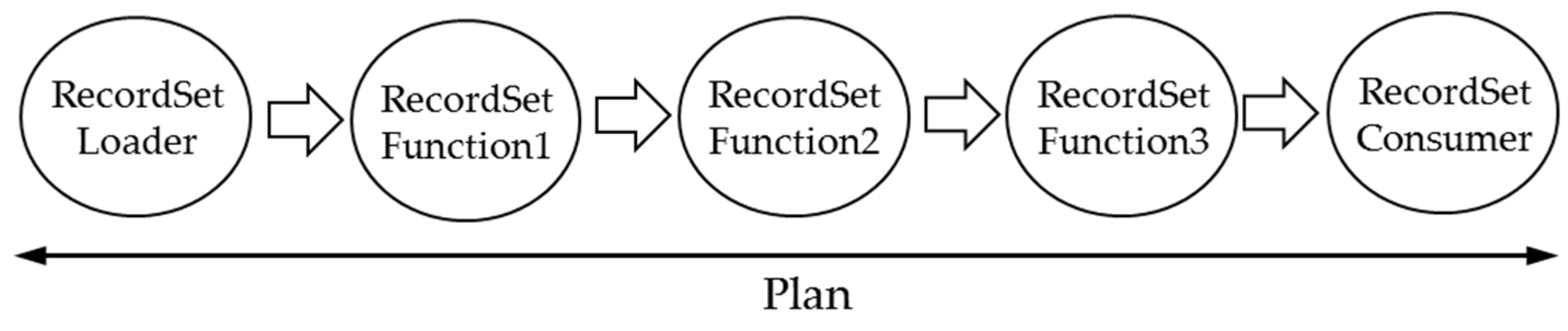
Spatial analysis is the process of investigating the positions, attributes, or relationships of objects based on spatial data to obtain valuable knowledge or to answer a question. In Marmot, spatial analysis using big data is defined as a chain of one or more units of RecordSetOperators, called a Plan. In a Plan, a RecordSetLoader and a RecordSetConsumer are generally placed in the first and last position, respectively; each RecordSetFunction is placed in the middle of the Plan. In order to process a given Plan, Marmot sequentially processes each RecordSetOperator comprising the Plan.
Figure 6 shows an example of a Plan consisting of a total of five RecordSetOperators: one RecordSetLoader, three RecordSetFunctions, and one RecordSetConsumer. As mentioned in the previous section, the RecordSetLoader transforms external geospatial big data into an internal form of Marmot which is a RecordSet. Then, one or more numbers of RecordSetFuntions process the RecordSet and create a new RecordSet containing the desired contents. Finally, the RecordSetConsumer stores the result in the output files on the file system.
5.2. Mapping a Plan to a Sequence of MapReduce Jobs
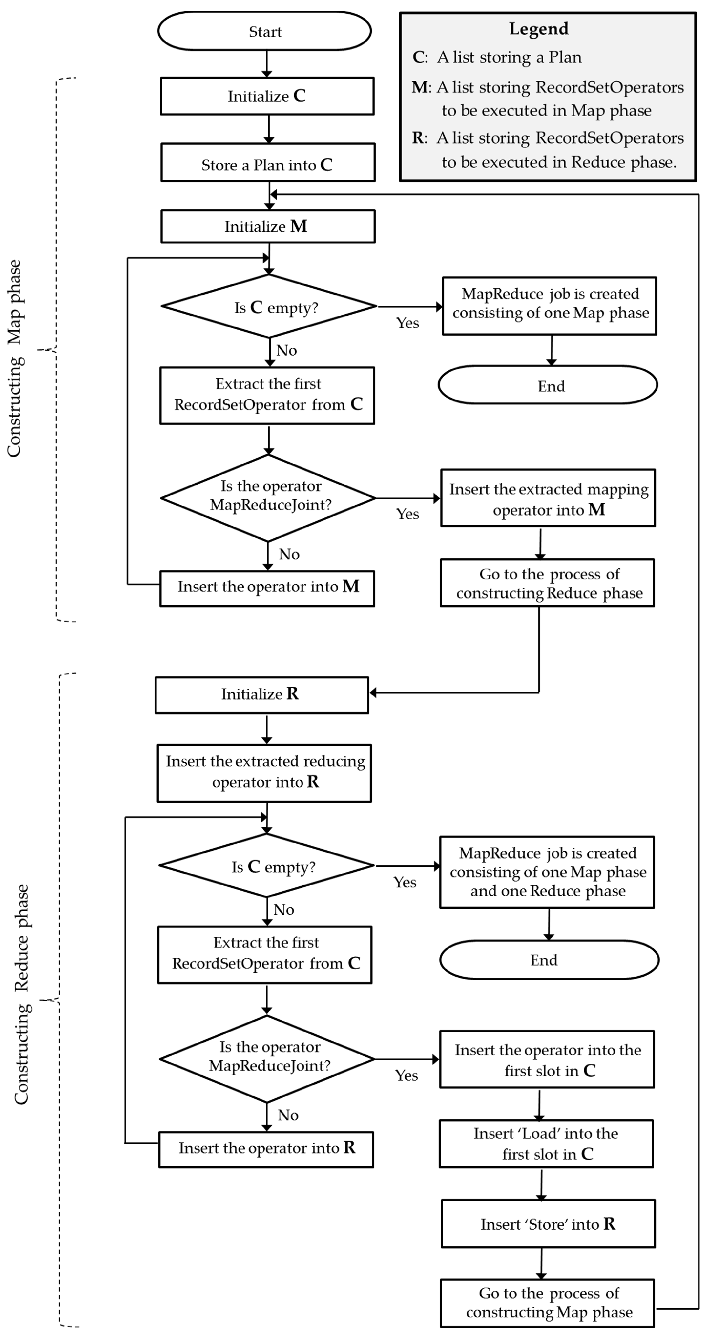
Marmot receives a Plan and automatically constructs one or more MapReduce jobs based on the features of each of the RecordSetFunctions. In general, to create a MapReduce job for a required operation in Hadoop, a programmer needs to specify both a map function and a reduce function. A spatial analysis task usually requires multiple MapReduce jobs to achieve a result, thereby making it cumbersome to write iterative code to describe complex MapReduce workflows [31]. The main idea of Marmot is to provide advantages which enable developers that have no detailed knowledge of MapReduce to build high performance geospatial analysis applications by simply combining built-in RecordSetFuntions. The specific process of mapping a Plan to a sequence of MapReduce jobs is described in Figure 7.
In Marmot, operators in RecordSetFuntions are classified into one of three categories: MapReduceTerminal, MapReduceJoint, or neither, depending on their own features. The term MapReduceTerminal implies operators not generating a RecordSet as the result of their executions; operators involved in RecordSetConsumer (e.g., storeAsCsv) usually belong to this category. The term MapReduceJoint is defined as those operators in RecordSetFuntions generating a RecordSet after grouping input data based on specific columns and then processing the grouped data. Aggregation operators (e.g., GroupBy) performing an operation on a given set of values and returning a RecordSet usually belong to this category. Lastly, there are operators in RecordSetFuntions not involved in either MapReduceTerminal or MapReduceJoint—most operators belong to this category. Among the three categories, MapReduceJoint is an important separation point to produce the Map phase and Reduce phase. An example of MapReduceTerminal and MapReduceJoint is shown in Table 2.
The process of mapping a Plan to a sequence of MapReduce jobs, specified in Figure 7, is as follows. When Marmot receives a Plan from an analysis application, Marmot extracts the first RecordSetOperator from the Plan and checks whether the operator belongs to the category of MapReduceJoint. If the operator does not belong to MapReduceJoint, Marmot inserts it in a separate list storing RecordSetOperators to be executed in Map phase (i.e., M in Figure 7) and extracts the next RecordSetOperator. This process is repeated until the last RecordSetOperator is inserted into the M then, finally, a MapReduce job is created consisting of only one Map phase.
During the process of constructing M when Marmot finds an operator belonging to MapReduceJoint, it constructs another list which is a set of RecordSetOperators to be executed in Reduce phase (i.e., R in Figure 7). The specific procedure of constructing R is as follows. Marmot decomposes the operator belonging to MapReduceJoint and extracts two suboperators: the mapping operator and reducing operator. For example, in the case of PickTopK which is one of the RecordSetOperators in MapReduceJoint, Sort (cols) and Take (k) are mapping and reducing operators of PickTopK, respectively. The extracted mapping operator is attached at the end of M and the reducing operator is inserted into the initialized R.
Marmot then extracts the next RecordSetOperator from the Plan and resumes examining whether the operator belongs to the category of MapReduceJoint. If the operator belongs to MapReduceJoint, Marmot inserts it in R and extracts the next RecordSetOperator. This process is repeated until the last RecordSetOperator is inserted in the R; then finally a MapReduce job is created consisting of one Map phase and one Reduce phase. During the process of constructing R, when Marmot meets an operator belonging to MapReduceJoint, Marmot iteratively constructs another MapReduce job by treating the remaining RecordSetOperators as a new Plan.
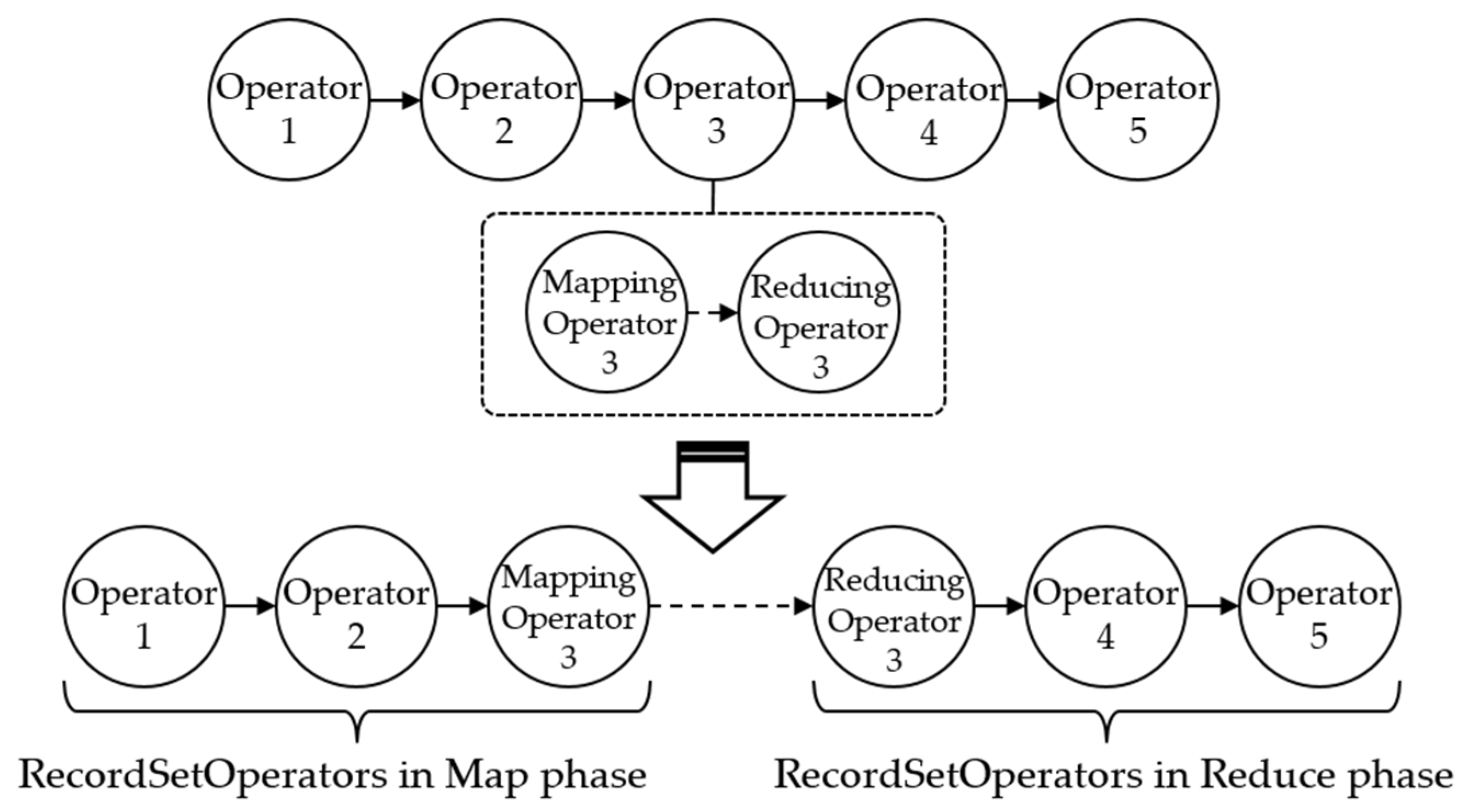
Figure 8 shows an example of the process of creating MapReduce jobs in Marmot. The given Plan in the example consists of five RecordSetOperators where operator3 is the only operator belonging to MapReduceJoint. During the process, operator3 is decomposed into two operators—a mapping operator and reducing operator. The Plan is eventually transformed into MapReduce jobs consisting of several map tasks and reduce tasks. Each map task performs operator1 and operator2 and the reduce tasks perform operator4 and operator5. Operator3, which is defined as a MapReduceJoint, is broken down into two suboperators and they are carried out at map tasks and reduce tasks, respectively. The number of map tasks is heavily dependent on the size of the input dataset. In the default configuration, each map task takes care of 64MB of input dataset. The number of reduce tasks is, however, is usually decided by the parameters of the MapReduceJoint operator, which is operator3 in this example.
Although Marmot has been built on a CentOS 6.9 environment, it can easily be executed on any operating system where Hadoop is installed due to the characteristics of Java’s platform independency. As a Hadoop system, Marmot uses Hortonworks Data Platform (HDP) 2.6 version. Table 3 shows the specific environment of implementation and testing of Marmot.
6. Case Analysis: Subway Stations
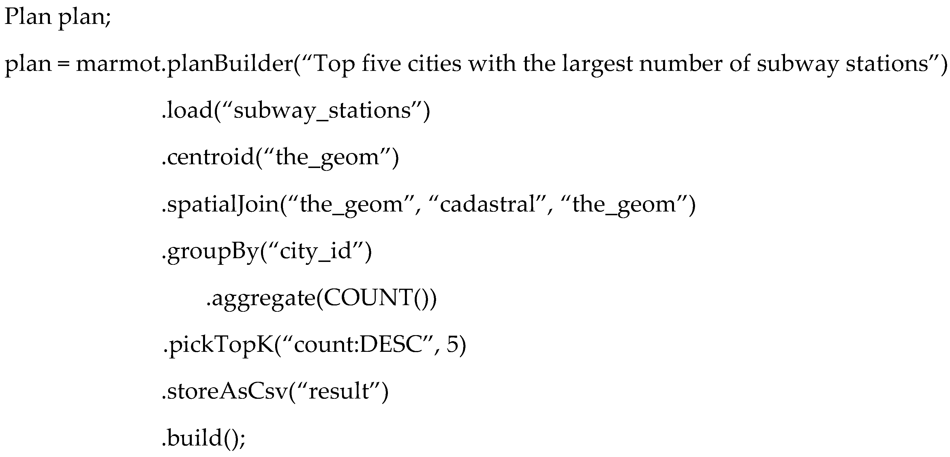
To show how Marmot handles geospatial big data, this section presents an example of spatial analysis. Figure 9 is a sample code of a Plan retrieving the number of subway stations per city. For this analysis, nationwide datasets of cadastral and subway stations in Korea are used.
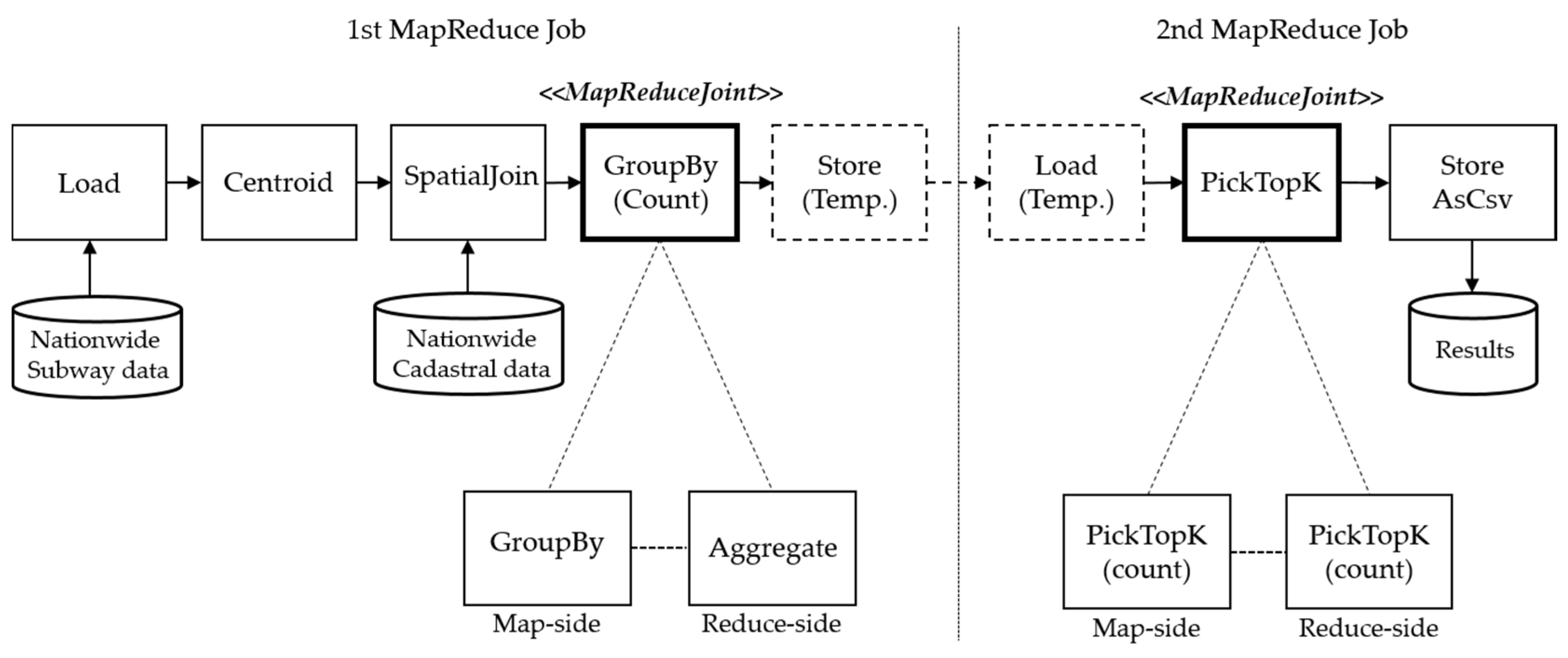
The plan is composed of six RecordSetOperators: ‘Load’, ‘Centroid’, ‘SpatialJoin’, ‘GroupBy’, ‘PickTopK’, and ‘StoreAsCsv’. As shown in Figure 10, using the ‘Load’ operator, Marmot reads the boundaries of each subway station and ‘Centroid’ operator computes their center coordinates. With the ‘SpatialJoin’ operator, Marmot finds a city whose boundary contains the centroid of each subway station. Then, the ‘GroupBy’ operator groups the output records based on each city and counts the number of their records. The output records should be ‘(city_id, count)’ pairs, which contain the number of subway stations for each city. Finally, the ‘PickTopK’ operator sorts the record on the basis of numbers and picks the top five cities. These five records are stored in the Hadoop Distributed File System (HDFS) by the ‘StoreAsCsv’ operator.
In the process of transforming the Plan to a sequence of MapReduce jobs, Marmot recognizes two ‘MapReduceJoint’ operators: ‘GroupBy’ and ‘PickTopK’. Since each ‘MapReduceJoint’ generates one MapReduce job, the plan is transformed into two separate MapReduce jobs, as depicted in Figure 10. For the first MapReduce job, the ‘GroupBy’ operator is the breakpoint producing the first Map and Reduce tasks, and ‘PickTopK’ operator is another breakpoint to produce the second MapReduce job. The output of the first MapReduce job is stored in a temporary HDFS file—so that the second MapReduce job can continue to execute the rest of the given Plan. Marmot deletes the temporary file when the whole plan has been executed.
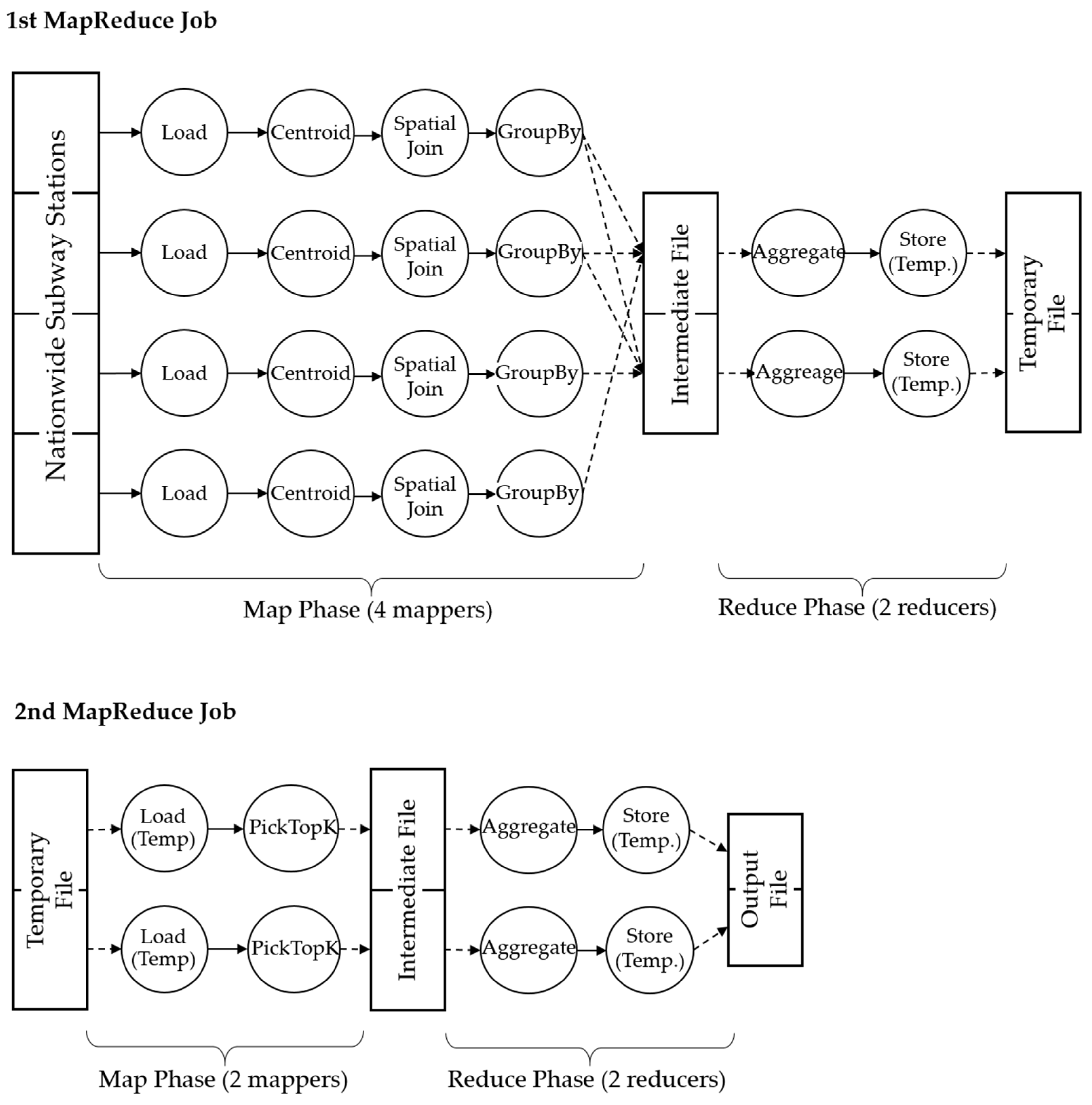
The sequence of RecordSetOperators assigned during Map and Reduce phases is executed in a pipeline manner by a number of mappers and reducers. The number of mappers is dynamically determined by the size of input data whereas the number of reducers is statically fixed in a Plan. During the process of a given analysis, four mappers with two reducers are used in the first MapReduce job and two mappers with two reducers are used in the second MapReduce job, as shown in Figure 11.
7. Experiments
7.1. Test Cases
Experiments were conducted to compare the performance of Marmot to that of SpatialHadoop, one of the top MapReduce frameworks supporting spatial functionalities. Since the geospatial operators currently supported by SpatialHadoop are limited compared to Marmot, it is difficult to conduct our experiments based on complex spatial analysis tasks. Therefore, we decided to perform a comparison for each of the fundamental spatial operations supported by both SpatialHadoop and Marmot.
There are five target spatial operations in our experiments: obtaining minimum bounding rectangle (MBR) and creating spatial index, range query without index, range query with index, and spatial join with index. MBR has been most commonly used to approximate spatial objects and is one of the fundamental operations for spatial analysis. A query for obtaining MBRs is therefore included in our experiment. Spatial index also plays an important role in geospatial domain to speed up retrieving certain objects in a spatial database, making measuring the performance of creating spatial index essential for this evaluation. Range query allows one to search for spatial objects located in a specified spatial extent and is therefore a fundamental type of query in spatial databases. To see the impact of using spatial index on range query performance, we investigated two cases—with and without an index. Lastly, spatial join is one of the most important operations for combining spatial objects and serves as building blocks for processing complex spatial analysis. Even with the support of spatial index, spatial join is particularly complex and time-intensive. Thus, efficient processing of spatial join is crucial to increase query performance.
7.2. Data Description
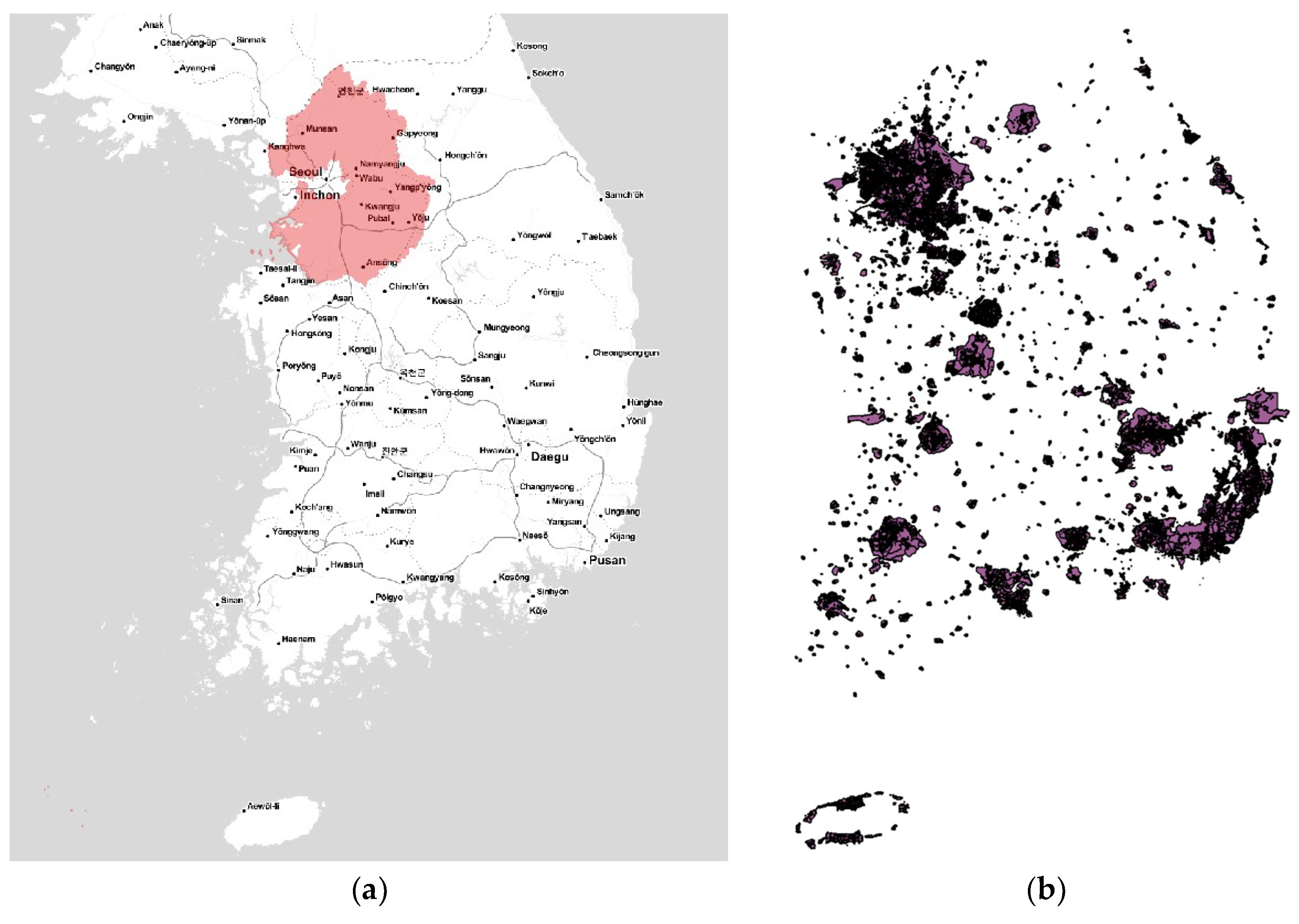
For the experiment, we used two Tiger Files including real spatial data for Korea. One file contained a nationwide continuous cadastral map with a size of 16GB (38,744,510 polygons); the other file included major urban areas created for management of land use with a size of 0.3GB (53,087 polygons). Figure 12 shows the visualization of these two Tiger Files including real spatial datasets of Korea. Particularly, Figure 12a shows just part of the continuous cadastral map because the entire data are too large to load onto the visualization tool. To demonstrate what all the data look like, partial data with a size of 1.24GB (4,720,616 polygons) involving Seoul city and Gyeonggi Province are plotted using red on a grayscale OSM basemap as the one by Stamen.
Of the five test cases in our experiment, three cases (i.e., obtaining MBR, range query without index, and range query with index) use only the cadastral data; one case (i.e., creating spatial index) uses only the major urban data and one case (i.e., spatial join) uses both the cadastral and major urban data.
7.3. Results
Each test query was run five times and the average, after excluding the highest and lowest values, was chosen to evaluate performance. The formula to express the performance improvement rate (PIR) of Marmot is:
where SH and M are execution times required by SpatialHadoop and Marmot, respectively. Table 4 shows the execution time of each test case and the PIR.
PIR = ((SH – M)/M) * 100
In designing the experiment, we included only fundamental spatial operations due to the infrastructural limits of SpatialHadoop. Although SpatialHadoop has built-in spatial analytic functions, it supports few spatial operations and lacks many useful functions such as coordinate conversation, exporting spatial data, and raster processing functions. In addition, SpatialHadoop was not designed to read Shapefiles directly, which is a very popular geospatial vector data format used in spatial domain. Instead, SpatialHadoop reads spatial data represented in well-known text (WKT) or well-known binary (WKB). Because of this, in this paper we focused on measuring only the performance of fundamental spatial operations.
In all five test cases, Marmot outperforms SpatialHadoop with a variation depending on the type of test. In the case of simple operations such as range query, the performance difference between SpatialHadoop and Marmot is small (PIR = 5% for range query without index). However, in the case of complex operations especially involving spatial index, Marmot highly outperforms SpatialHadoop (PIR = 209% for range query with index; PIR = 72% for spatial join with index). This is because those operations are strongly influenced by the performance of spatial index and Marmot greatly outperforms SpatialHadoop in these operations (PIR = 132% for creating spatial index). Lastly, in the case of creating MBR that is an essential prerequisite for creating spatial index, Marmot also has a higher performance than SpatialHadoop (PIR = 301% for creating MBR).
8. Discussion
Marmot has been developed as one component for constructing a national geospatial big data platform [4] promoted by the Ministry of Land, Infrastructure, and Transport of the Korean government. Marmot is publicly available including GitHub [32] and will be integrated into other components of the platform to be used for public services such as transport, real estate, or disaster prevention. Based on the long-term plans of the Korean government to promote the geospatial industry, Marmot also will be integrated with the national geospatial information open platform, V-World [33], to provide a variety of map-based spatial analysis services. In addition, other ministries dealing with spatial data also plan to use Marmot as an infrastructure platform to provide big data based analysis services.
Compared to existing systems, Marmot is distinguished by the following. First, Marmot supports seamless integration between spatial and nonspatial operations within a solid framework, thereby improving workflow performance. Second, Marmot outperforms existing top-tier, plug-in based, spatial big data frameworks, especially for complex and time-intensive queries involving a spatial index. Third, Marmot provides a variety of spatial operators, which allow executing further complex spatial analyses. Finally, once application developers recognize a set of nonspatial and spatial operators, they can implement desired spatial analysis tasks without having to possess detailed knowledge of big data technologies.
Although Marmot shows good performance results compared to other existing research, it still needs further improvement. First, Marmot is restricted to batch processing only. Batch processing is efficient for handling huge amounts of data, but outcomes can be delayed depending on the input data size and computing power of a machine. Many recent geospatial data analytics require real-time data processing; however, Marmot does not yet support real-time processing of streamed data. Second, many machine learning algorithms read modestly sized source datasets iteratively, e.g., K-means and DBSCAN. For those applications, in-memory data processing offers the best match, but the current version of Marmot lacks this. Although Marmot utilizes memory, in part, along with disks during data processing [34], it cannot take full advantage of in-memory computation to increase processing speed.
In the future, we first plan to investigate what additional factors create performance differences between Marmot and SpatialHadoop and conduct extensive experiments using more large-scale geospatial big data. Second, we are going to finalize implementing an Apache Spark-based geospatial big data processing system, which is currently underdeveloped. To address the aforementioned limitations of Marmot, we have selected Spark as a framework for our next system for analyzing geospatial big data since Spark supports both in-memory and real-time data processing. Finally, we will design and conduct experiments comparing performance between Marmot and the new system.
9. Conclusions
The majority of existing NoSQL systems supporting geospatial data processing on Hadoop embed spatial functions as a form of plug-in to support extra features within their systems. This plug-in based approach suffers from severe performance problems due to the massive volume of data transfer between NoSQL and spatial plugins. In order to reduce data-transfer overhead, we have developed a new geospatial data processing framework on Hadoop, named Marmot. Marmot executes both spatial operations and nonspatial operations in the same session to avoid massive data transfer between operations, and employs a new method that maps a sequence of operations, either spatial or nonspatial, into a series of MapReduce jobs. We also show the proposed method outperforms SpatialHadoop with performance experiments.
Author Contributions
Kang-Woo Lee designed and implemented Marmot; Kang-Woo Lee and Junghee Jo conducted the testing of Marmot and analyzed the results; Junghee Jo wrote the manuscript; and Kang-Woo Lee revised the manuscript.
Acknowledgments
This research, “Geospatial Big Data Management, Analysis, and Service Platform Technology Development”, was supported by the MOLIT (The Ministry of Land, Infrastructure, and Transport), Korea, under the National Spatial Information Research Program supervised by the KAIA (Korea Agency for Infrastructure Technology Advancement) (18NSIP-B081011-05).
Conflicts of Interest
The authors declare no conflicts of interest.
References
- Yang, C.; Liu, C.; Zhang, X.; Nepal, S.; Chen, J. A time efficient approach for detecting errors in big sensor data on cloud. IEEE Trans. Parallel Distrib. Syst. 2015, 26, 329–339. [Google Scholar] [CrossRef]
- Ang, L.M.; Seng, K.P.; Zungeru, A.; Ijemaru, G. Big sensor data systems for smart cities. IEEE Internet Things J. 2017, 4, 1259–1271. [Google Scholar] [CrossRef]
- Li, S.; Dragicevic, S.; Castro, F.A.; Sester, M.; Winter, S.; Coltekin, A.; Pettit, C.; Jiang, B.; Haworth, J.; Stein, A.; et al. Geospatial big data handling theory and methods: A review and research challenges. ISPRS J. Photogramm. Remote Sens. 2016, 115, 119–133. [Google Scholar] [CrossRef] [Green Version]
- Lee, J.G.; Kang, M. Geospatial big data: Challenges and opportunities. Big Data Res. 2015, 2, 74–81. [Google Scholar] [CrossRef]
- Amirian, P.; Van Loggerenberg, F.; Lang, T.; Varga, M. Geospatial big data for finding useful insights from machine data. In GISResearch UK; University of Leeds: Leeds, United Kingdom, 2015. [Google Scholar]
- Morais, C.D. Where is the Phrase “80% of Data is Geographic” From? Available online: http://www.gislounge.com/80-percent-data-is-geographic (accessed on 4 April 2018).
- Jeansoulin, R. Review of forty years of technological changes in geomatics toward the big data paradigm. ISPRS Int. J. Geo-Inf. 2016, 5, 155. [Google Scholar] [CrossRef]
- He, Z.; Liu, Q.; Deng, M.; Xu, F. March. Handling multiple testing in local statistics of spatial association by controlling the false discovery rate: A comparative analysis. In Proceedings of the 2017 IEEE 2nd International Conference Big Data Analysis (ICBDA), Beijing, China, 10–12 March 2017; pp. 684–687. [Google Scholar]
- Seethapathy, B.K.; Parvathi, R. A review on spatial big data analytics and visualization. In Modern Technologies for Big Data Classification and Clustering; IGI Global: Philadelphia, PA, USA, 2017; p. 179. ISBN 978-1522528050. [Google Scholar]
- Carpenter, J.; Snell, J. Future Trends in Geospatial Information Management: The Five to Ten Year Vision. United Nations Initiative on Global Geospatial Information Management. Available online: http://ggim.un.org/ggim_20171012/docs/meetings/GGIM5/Future%20Trends%20in%20Geospatial%20Information%20Management%20%20the%20five%20to%20ten%20year%20vision.pdf (accessed on 4 April 2018).
- Vatsavai, R.R.; Ganguly, A.; Chandola, V.; Stefanidis, A.; Klasky, S.; Shekhar, S. Spatiotemporal data mining in the era of big spatial data: Algorithms and applications. In Proceedings of the 1st ACM SIGSPATIAL International Workshop on Analytics for Big Geospatial Data, Redondo Beach, CA, USA, 7–9 November 2012; pp. 1–10. [Google Scholar]
- Dasgupta, A. Big Data: The Future is in Analytics. Available online: https://www.geospatialworld.net/article/big-data-the-future-is-in-analytics (accessed on 20 April 2018).
- Maguire, D.J.; Longley, P.A. The emergence of geoportals and their role in spatial data infrastructures. Comput. Environ. Urban Syst. 2005, 29, 3–14. [Google Scholar] [CrossRef]
- Annoni, A.; Bernard, L.; Fullerton, K.; de Groof, H.; Kanellopoulos, I.; Millot, M.; Peedell, S.; Rase, D.; Smits, P.; Vanderhaegen, M. Towards a European spatial data infrastructure: The INSPIRE initiative. In Proceedings of the 7th International Global Spatial Data Infrastructure Conference, Bangalore, India, 2–6 February 2004. [Google Scholar]
- Bernard, L.; Kanellopoulos, I.; Annoni, A.; Smits, P. The European geoportal—One step towards the establishment of a European Spatial Data Infrastructure. Comput. Environ. Urban Syst. 2005, 29, 15–31. [Google Scholar] [CrossRef]
- Busby, J.R.; Kelly, P. Australian spatial data infrastructures. In Proceedings of the 7th International Global Spatial Data Infrastructure Conference, Bangalore, India, 2–6 February 2004. [Google Scholar]
- Sivakumar, R.; Rao, M.; Dasgupta, A.R. Perspectives of India’s national spatial data infrastructure. In Proceedings of the 7th International Global Spatial Data Infrastructure Conference, Bangalore, India, 2–6 February 2004. [Google Scholar]
- Dewitt, D.; Gray, J. Parallel database system: The future of high performance database systems. Commun. ACM 1992, 35, 85–98. [Google Scholar] [CrossRef]
- White, T. Hadoop: The Definitive Guide, 3rd ed.; O’Reilly Media: Newton, MA, USA, 2012; ISBN 1449338771. [Google Scholar]
- GitHub. Available online: http://esri.github.io/gis-tools-for-hadoop (accessed on 10 May 2018).
- Aji, A.; Wang, F.; Vo, H.; Lee, R.; Liu, Q.; Zhang, X.; Saltz, J. Hadoop-GIS: A high performance spatial data warehousing system over MapReduce. In Proceedings of the VLDB Endowment 2013, Trento, Italy, 26–30 August 2013; pp. 1009–1020. [Google Scholar]
- Gao, S.; Li, L.; Li, W.; Janowicz, K.; Zhang, Y. Constructing gazetteers from volunteered big geo-data based on Hadoop. Comput. Environ. Urban Syst. 2017, 61, 172–186. [Google Scholar] [CrossRef]
- Eldawy, A. SpatialHadoop: Towards flexible and scalable spatial processing using mapreduce. In Proceedings of the SIGMOD PhD Symposium 2014, Snowbird, UT, USA, 22–27 June 2014; ACM: New York, NY, USA; pp. 46–50. [Google Scholar]
- Eldawy, A.; Mokbel, M.F. SpatialHadoop: A MapReduce framework for spatial data. In Proceedings of the 2015 IEEE 31st International Conference Data Engineering (ICDE), Seoul, South Korea, 13–17 April 2015; pp. 1352–1363. [Google Scholar]
- Dean, J.; Ghemawat, S. MapReduce: Simplified data processing on large clusters. Commun. ACM 2008, 51, 107–113. [Google Scholar] [CrossRef]
- Zaharia, M.; Chowdhury, M.; Franklin, M.J.; Shenker, S.; Stoica, I. Spark: Cluster computing with working sets. In Proceedings of the 2nd USENIX Conference on Hot Topics in Cloud Computing, Boston, MA, USA, 21–25 June 2010. [Google Scholar]
- Agarwal, S.; Rajan, K.S. Analyzing the performance of NoSQL vs. SQL databases for Spatial and Aggregate queries. In Proceedings of the Free and Open Source Software for Geospatial (FOSS4G) Conference 2017, Boston, MA, USA, 14–19 August 2017. [Google Scholar]
- Brahim, M.B.; Drira, W.; Filali, F.; Hamdi, N. Spatial data extension for Cassandra NoSQL database. J. Big Data 2016, 3, 11. [Google Scholar] [CrossRef]
- Vasavi, S.; Priya, M.P.; Gokhale, A.A. Framework for Geospatial Query Processing by Integrating Cassandra with Hadoop. Knowl. Comput. Appl. 2018, 131–160. [Google Scholar] [CrossRef]
- Eldawy, A.; Mokbel, M.F. The ecosystem of SpatialHadoop. SIGSPATIAL Spec. 2015, 6, 3–10. [Google Scholar] [CrossRef]
- Manoochehri, M. Data Just Right: Introduction to Large-Scale Data & Analytics; Addison-Wesley: Boston, MA, USA, 2013; ISBN 978-0133359077. [Google Scholar]
- Marmot from GitHub. Available online: https://github.com/kwlee0220/marmot.server.dist (accessed on 29 September 2018).
- Ministry of Land, Infrastructure and Transport in Korea, V-World. Available online: http://eng.vworld.kr/eng/em_main.do (accessed on 15 September 2018).
- Jo, J.H.; Lee, K.W. Marmot: A Hadoop-based high performance data storage management system for processing geospatial or geo-spatial big data. Korean Soc. Geospat. Inf. Sci. 2018, 26, 3–10. [Google Scholar]
Figure 1.
Overall structure of Marmot.

Figure 2.
Comparison of two Hadoop-based architectures integrating spatial and nonspatial operations: (a) Plug-in based NoSQL system and (b) Marmot.
Figure 2.
Comparison of two Hadoop-based architectures integrating spatial and nonspatial operations: (a) Plug-in based NoSQL system and (b) Marmot.

Figure 3.
An overall description of a data model in Marmot.

Figure 4.
A description of a RecordSetOperator in Marmot: RecordSetLoader, RecordSetFuntion, and RecordSetConsumer.
Figure 4.
A description of a RecordSetOperator in Marmot: RecordSetLoader, RecordSetFuntion, and RecordSetConsumer.

Figure 5.
A Marmot code of an example of RecordSetLoader and RecordSetConsumer.

Figure 6.
A description of a Plan in Marmot: A chain of RecordSetOperators.

Figure 7.
An algorithm of automatic mapping a Plan to a sequence of MapReduce jobs in Marmot. C refers to a list storing a Plan; M refers to a list storing RecordSetOperators to be executed in Map phase; and R refers to a list storing RecordSetOperators to be executed in Reduce phase.
Figure 7.
An algorithm of automatic mapping a Plan to a sequence of MapReduce jobs in Marmot. C refers to a list storing a Plan; M refers to a list storing RecordSetOperators to be executed in Map phase; and R refers to a list storing RecordSetOperators to be executed in Reduce phase.

Figure 8.
An example of transforming a Plan to a sequence of MapReduce jobs in Marmot.

Figure 9.
A Marmot code of an example Plan retrieving the top five cities with the largest number of subway stations.
Figure 9.
A Marmot code of an example Plan retrieving the top five cities with the largest number of subway stations.

Figure 10.
A sequence of RecordSetOperators consisting of the example Plan.

Figure 11.
Operations in Map and Reduce phases in the first and second MapReduce jobs.

Figure 12.
Visualization of two Tiger Files including real spatial datasets of Korea. (a) Part of the continuous cadastral map (1.24GB out of 16GB; 4,720,616 polygons out of 38,744,510 polygons) plotted using red and (b) major urban areas (0.3GB, 53,087 polygons) created for management of land use.
Figure 12.
Visualization of two Tiger Files including real spatial datasets of Korea. (a) Part of the continuous cadastral map (1.24GB out of 16GB; 4,720,616 polygons out of 38,744,510 polygons) plotted using red and (b) major urban areas (0.3GB, 53,087 polygons) created for management of land use.


Table 1.
Spatial and nonspatial operators in RecordSetFuntion supporting in Marmot.
| Spatial operators | Nonspatial operators |
|---|---|
| Buffer, Centroid, TransformCRS, Dissolve, LookupPostalAddress, AggrUnion, AggrConvexHull, Intersection, SpatialJoin, SpatialOuterJoin, SpatialSemiJoin, kNNJoin, ClipJoin, DifferenceJoin, AggregateJoin, LoadSpatialIndexJoin, AggrEnvelope, RangeQuery, EstimateIDW, GetisOrd, EstimateKernelDensity, LocalMoran’s I, E2SFCA | Filter, Project, Update, Transform, Skip, Distinct, Rank, PickTopK, Aggregate, GroupBy, Shard, Sample, Sort, Limit, Reduce, MapReduceEquiJoin, ReduceByGroupKey |
Table 2.
RecordSetOperators classified as MapReduceTermial and MapReduceJoint, repectively.
| MapReduceTerminal | MapReduceJoint |
|---|---|
| storeMarmotFile, store, storeAsCsv | MapReduceEquiJoin, PickTopK, ReduceByGroupKey |
Table 3.
Implementation and testing environment for Marmot.
| Software | Version |
|---|---|
| CentOS | 6.7 |
| Hortonworks Data Platform | 2.6 |
| JDK | 1.8 |
| PostgreSQL | 9.4.7 |
Table 4.
A comparison of execution time and performance improvement rate (PIR) (in seconds).
| Geospatial operators | SpatialHadoop | Marmot | PIR |
|---|---|---|---|
| Create MBR | 81.634 | 20.336 | 301% |
| Create spatial index | 220.494 | 95.220 | 132% |
| Spatial join with index | 21.841 | 12.688 | 72% |
| Range query with index | 2.836 | 0.918 | 209% |
| Range query without index | 17.827 | 16.972 | 5% |
© 2018 by the authors. Licensee MDPI, Basel, Switzerland. This article is an open access article distributed under the terms and conditions of the Creative Commons Attribution (CC BY) license (http://creativecommons.org/licenses/by/4.0/).
Share and Cite
MDPI and ACS Style
Jo, J.; Lee, K.-W. High-Performance Geospatial Big Data Processing System Based on MapReduce. ISPRS Int. J. Geo-Inf. 2018, 7, 399. https://doi.org/10.3390/ijgi7100399
AMA Style
Jo J, Lee K-W. High-Performance Geospatial Big Data Processing System Based on MapReduce. ISPRS International Journal of Geo-Information. 2018; 7(10):399. https://doi.org/10.3390/ijgi7100399
Chicago/Turabian StyleJo, Junghee, and Kang-Woo Lee. 2018. "High-Performance Geospatial Big Data Processing System Based on MapReduce" ISPRS International Journal of Geo-Information 7, no. 10: 399. https://doi.org/10.3390/ijgi7100399
Note that from the first issue of 2016, this journal uses article numbers instead of page numbers. See further details here.