Incremental Road Network Generation Based on Vehicle Trajectories


1
School of Aeronautics and Astronautics, Zhejiang University, Hangzhou 310027, China
2
Zhejiang Lab, Hangzhou 311121, China
*
Author to whom correspondence should be addressed.
ISPRS Int. J. Geo-Inf. 2018, 7(10), 382; https://doi.org/10.3390/ijgi7100382
Submission received: 11 August 2018
/
Revised: 20 September 2018
/
Accepted: 21 September 2018
/
Published: 23 September 2018
Abstract
:Nowadays, most vehicles are equipped with positioning devices such as GPS which can generate a tremendous amount of trajectory data and upload them to the server in real time. The trajectory data can reveal the shape and evolution of the road network and therefore has an important value for road planning, vehicle navigation, traffic analysis, and so on. In this paper, a road network generation method is proposed based on the incremental learning of vehicle trajectories. Firstly, the input vehicle trajectory data are cleaned by a preprocess module. Then, the original scattered positions are clustered and mapped to the representation points which stand for the feature points of the real roads. After that, the corresponding representation points are connected based on the original connection information of the trajectories. Finally, all representation points are connected by a Delaunay triangulation network and the real road segments are found by a shortest path searching approach between the connected representation point pairs. Experiments show that this method can build the road network from scratch and refine it with the input data continuously. Both the accuracy and timeliness of the extracted road network can continuously be improved with the growth of real-time trajectory data.
1. Introduction
Street maps and transportation networks are the bases of building smart cities. High accurate road network maps have great social and application values. Currently, road network generating and updating algorithms can be mainly divided into three categories.
(i) Field measurement based on the professional GPS equipment and surface measurement technology [1]: This method relies on the professional road measurement vehicles and data collection personnel. It suffers the disadvantages of long work cycle, unstable measurement accuracy, high cost, expensive to maintain, etc. With the development of the satellite technology, its application range becomes even smaller.
(ii) Extracting road network map from remote sensing image based on the image processing technologies [2,3,4]: This method relies on remote sensing. However, high-definition remote sensing maps have low real-time performance and high purchase costs. They are limited by the image processing technology and are difficult to automate. Therefore, the extraction efficiency is relatively low.
(iii) Building the road network with Volunteered Geographic Information (VGI) [5]: This method relies on VGI, which is the harnessing of tools to create, assemble, and disseminate geographic data provided voluntarily by individuals. Thus, the quality of the updated map depends on the skill level of the volunteer and the accuracy of the data.
In recent years, with the rapid development of global positioning systems (GPS), radio frequency identification technologies (RFID), and sensor technologies, it has become easier to collect the location information of moving objects. Nowadays, more and more cars have installed GPS devices to record the vehicle’s trajectory. These vehicles can generate tens of thousands of vehicle trajectory data every day. These vehicle trajectory data not only contain the laws of the vehicle’s movements and traffic congestion, but also reveal the shape of the road network and the rules of the road network’s evolution over time. Therefore, more and more researchers have begun to use vehicle trajectory data to generate and update the road network information.
The existing methods for constructing a road network using vehicle trajectory data can be roughly divided into three categories.
(i) Point clustering assumes that the input is a set of points and clusters the points together through different clustering methods to obtain a road network map [6,7,8,9,10,11]. Representative algorithms in this class include the following. Li et al. [8] proposed the use of spatial-linear clusters to infer road segments from GPS trajectories. Their algorithm can detect missing road and checking the correctness of existing road network through inferring road segments. Edelkamp et al. [9] clustered high precision DGPS trajectories to construct road network, and the center of each cluster is regarded as the lane center line. In [10], GPS points are converted into binary image by morphological operations. Then, the skeleton is extracted to construct road network. Chen et al. [11] proposed a map interface algorithm with accuracy guarantees based on detecting seed elements and connecting them subsequently.
(ii) Incremental track insertion uses the idea of map matching to gradually insert the trajectory into the initial map to construct a road network map [1,12,13,14]. Representative algorithms in this class include the following. Zhang et al. [12] combined the K-Means clustering with the Gaussian model to extract the centerline of the road and continuously refine existing road network. Bruntrup et al. [13] proposed a spatial-clustering based algorithm that allows incrementally generating a road network, but the algorithm requires high quality (sampling rate and positional accuracy) tracking data. Cao and Krumm [1] applied a custom clustering algorithm to group similar input trajectories together and then build up the road network incrementally. Ahmed et al. [14] proposed an incremental algorithm for the road network construction that matching of trajectories and map is achieved by Fréchet distance. Although this algorithm guarantees the local quality of the road network, it does not solve the basic connectivity problem.
(iii) Intersection linking determines the intersection through the motion characteristics (speed and direction) or point density of the vehicle, and then connects the intersections by interpolation [15,16]. Representative algorithms in this class include the following. Fathi and Krumm [15] introduced an intersection detector trained on ground truth data from an existing map. Firstly, they find the intersections using a classifier learned over the shape descriptors. Then, they connected the intersections with geometrically accurate road segments. Finally, they used the iterative closest point algorithm to optimize the position of each intersection. Karagiorgou et al. [16] proposed the Trace Bundle algorithm, which realizes the classification of the trajectory by intersection turning model, and using trajectory clustering to realize road network extraction.
In this work, an algorithm for incrementally learning vehicle trajectory data and generating a road network is proposed. The algorithm does not require the existing road network as the basis. It incrementally generates a road network by learning the position and timing information from the input vehicle trajectory. The road network graph has a high timeliness and can be continuously updated when the input trajectory changes.
The outline of the paper is depicted as follows. Section 1 describes a detailed analysis of the characteristics of the vehicle trajectory data and explains the advantages of using the vehicle trajectory data to extract the road network. Section 2 depicts the detailed specific implementation flow of the road network extraction method based on incremental learning. Section 3 shows the experimental results and comparative analysis. Finally, Section 4 discusses conclusions and future work.
2. Analysis of Characteristics of Vehicle Trajectory Data
A trajectory is a polyline in a multidimensional space formed by a series of sampling points that contain attributes such as geographical location and time, which are used to represent the positional change of an object over a period. Vehicle trajectory refers to the trajectory of a set of sampling points obtained by the vehicle-mounted GPS device in the journey. The sampling points of a vehicle trajectory generally contain attributes such as position, time, speed, and direction. High-quality vehicle trajectory data have important social and application values in solving social issues such as traffic congestion, traffic services improving, road environment monitoring, and energy shortages alleviating [17]. In this paper, the road network is extracted from the vehicle trajectory data mainly based on the following characteristics of the vehicle trajectory:
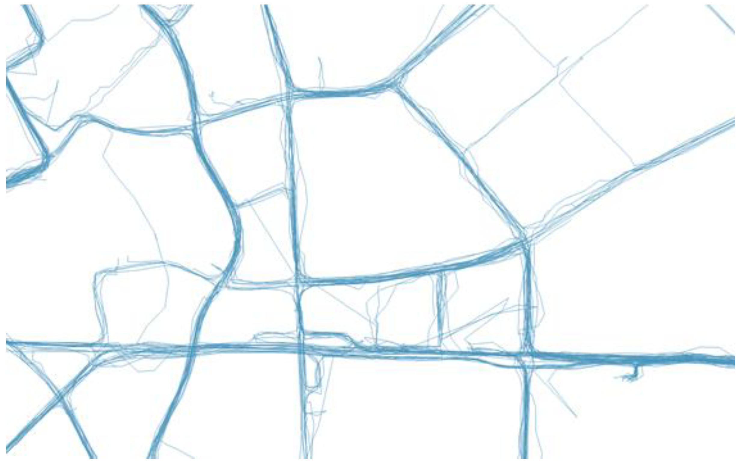
- The trajectory data express the information of road structure. The movement of a typical vehicle is always limited to the existing road network (the vehicle cannot move freely on the plane), so the vehicle trajectory data represent rich road structure information. In Figure 1, many vehicle trajectories are superimposed, roughly delineating the structure of the road network in the area.
- The real-time vehicle trajectory data express the dynamic changes of road status. With the rapid development of the city, urban roads are changing from time to time because of road construction, road maintenance, traffic control, etc. Therefore, high real-time performance is required for the road network extraction algorithm. The vehicle trajectories are determined by the road status which is always changing along with the road transformation. Therefore, it is a unique advantage to utilize the vehicle trajectory data to update the road network.
3. Extraction of Road Network by Incremental Learning Method
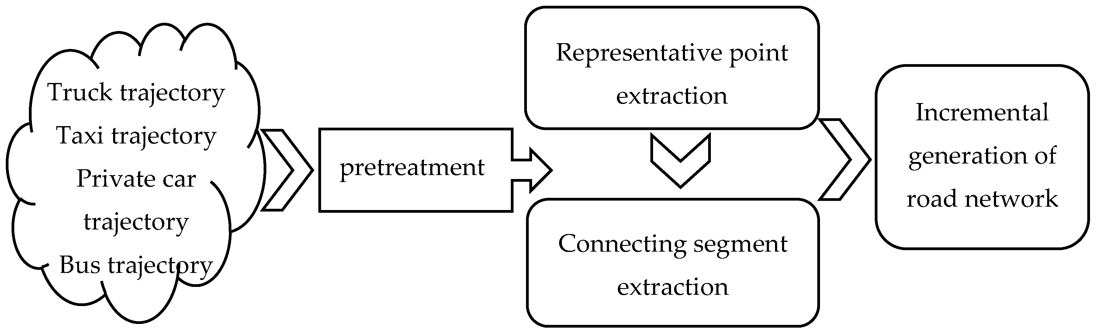
Figure 2 depicts the algorithm flow of incrementally learning from the vehicle trajectory data and building a road network. The algorithm has an input port to continuously receive trajectory data. Whenever a vehicle trajectory is obtained, firstly it will be pre-processed to ensure the correctness of the trajectory data. Then, the position information and timing information is learned from the input trajectory online. Finally, the road network is generated or updated incrementally based on the information.
In the following section, the four steps of the proposed algorithm, including trajectory data preprocessing, representative point extraction, connecting segment extraction and road network incremental generation, are described in detail.
3.1. Preprocessing of Vehicle Trajectory Data
Definition 1.
GPS point. The GPS point herein refers to the coordinate point of the vehicle position measured by the vehicle-mounted GPS device during the running of the vehicle. It is expressed as p = {x, y, t}, where x and y, respectively, correspond to the latitude and longitude of the vehicle location, which is measured by the positioning device, and t indicates the time when the vehicle is in this position.
Due to the limitations of the positioning accuracy and signal strength of the GPS device, there are usually a large number of errors and information missing in the original vehicle trajectory data. Therefore, it is necessary to preprocess the input vehicle trajectory data to repair or remove the abnormal data. Let , be two adjacent GPS points in a trajectory, where , . There are three typical cases on how the errors are introduced:
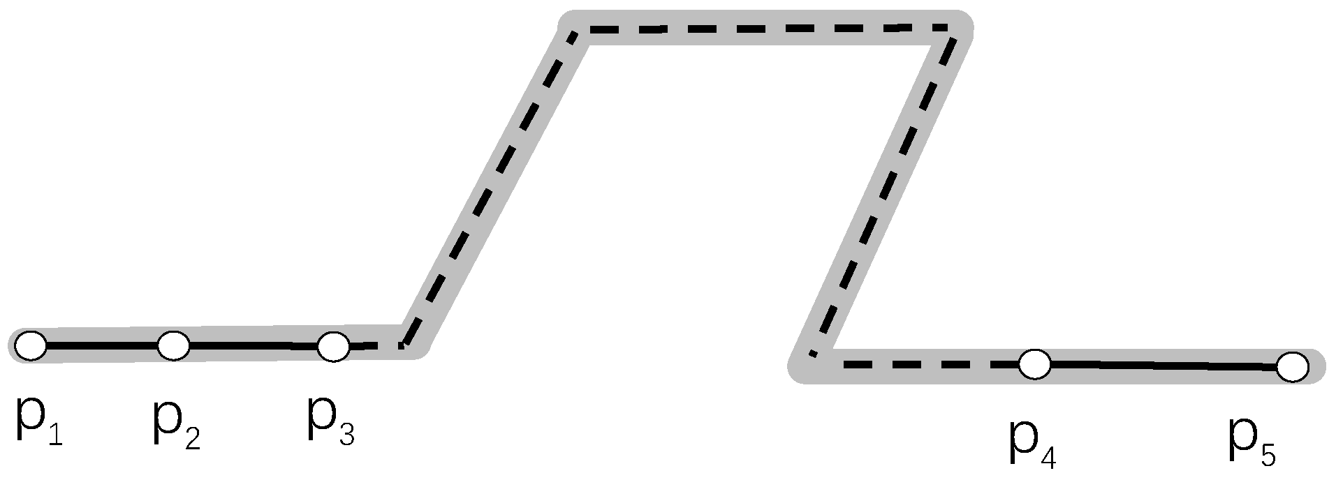
- When a vehicle is driving on the road, the signal of the GPS positioning equipment may be disturbed or interrupted because of the occlusion of trees, high buildings and other objects on both sides of the road, or vehicles entering tunnels, underground parking areas, etc., resulting in the interruption of the vehicle trajectory. Figure 3 depicts an example of such missing points. If p3 and p4 are directly connected, an erroneous trajectory will be formed. This work judges whether there are missing points in trajectory according to the time interval between two adjacent GPS points (), and discards the trajectory of a serious loss [18].
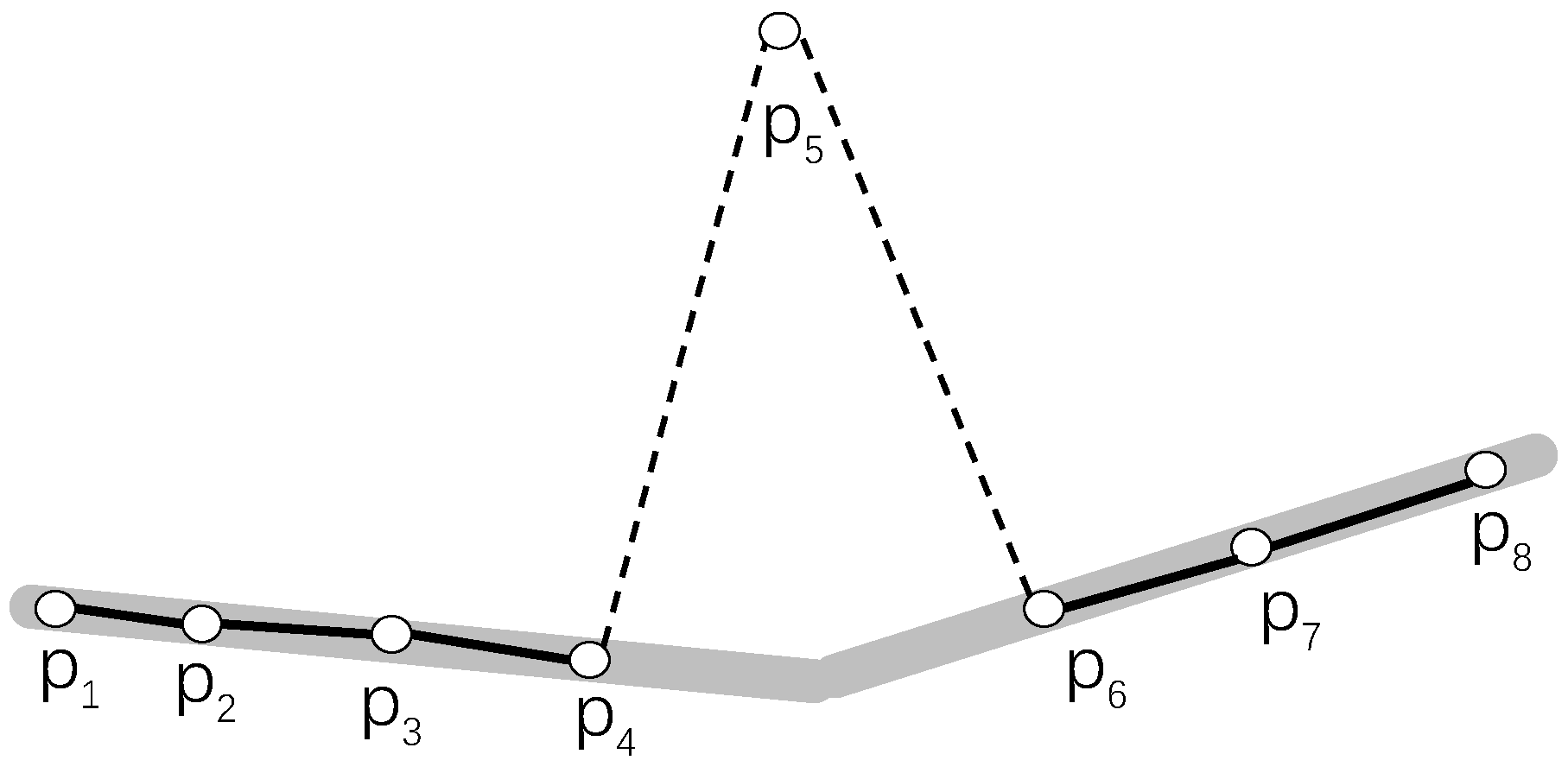
- The GPS device signal interference will additionally cause GPS positioning data to deviate from the actual vehicle driving routes and form noise points, as depicted in Figure 4. Noise points will affect the shape of the trajectories and make it fail to match the actual route. The noise points in the trajectory can be found and removed according to the average speed [18], which can be calculated by the distance and time interval between two adjacent GPS points ().
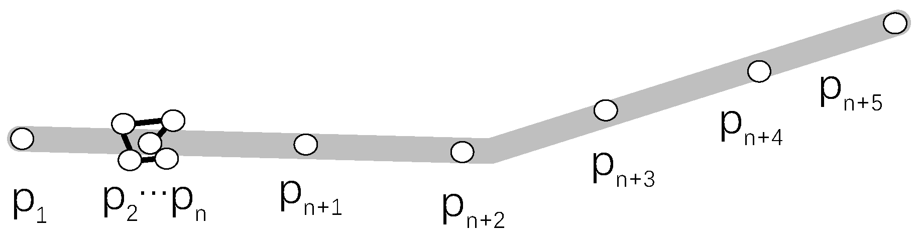
- When the vehicle is stopped, GPS devices may maintain working status. Therefore, there may be many same (similar) positioning points in the trajectory data during a long period of time. Such kind of points are called stationary points [18], as depicted in Figure 5. In the analysis of the road network structure, the stationary points in the vehicle trajectory will generate a large amount of data redundancy. The main feature of the stationary points is that the positions of consecutive GPS points keep still (or the change is small) (). This work uses this feature to find the stationary points in the trajectory and to delete the extra points [18].
3.2. Representative Point Extraction
The pre-processed trajectory has a shape that is close to the actual road. However, due to the GPS positioning accuracy, there is a certain deviation between the actual position and the positioning position of the vehicle, resulting in GPS positioning points scattered on both sides of the road. Therefore, the original vehicle track cannot be directly utilized as the road network segment. It should be noted that the positioning error here is obviously different from the noise point mentioned above. The noise point is a point that is completely irrelevant to the actual position of the vehicle because the GPS signal is disturbed, while the positional deviation caused by the positioning error is relatively smaller, and the position is closer to the actual position of the vehicle. Depending on the accuracy of GPS device, the range of the positioning error is various. In addition, the positioning frequency of different GPS devices is diverse, and the vehicle’s travel speed is varying under different traffic conditions. Therefore, there is a large difference in the distance between two adjacent GPS points. In more complex road sections or in morning and evening peak hours and other congested periods, the distances between adjacent GPS points are relatively smaller due to the slow speed of the vehicle, while the distances are relatively larger in relatively smooth road sections.
Definition 2.
Representative point. The n GPS points contained in a circle with a radius of R meters are represented by a representative point , where , , . , is the position of the point, n is the number of GPS points represented by the representative point, and t is the last update time of the representative point.
On the one hand, due to the error of the GPS positioning device, the measured vehicle position is usually equivalent to the actual position plus random Gaussian noise [19]. By extracting representative points from GPS points, the effects of such errors can be effectively eliminated, and the generated line segments can be closer to the center of the road. On the other hand, due to the different speeds of vehicles on different roads and the different positioning periods of different positioning devices, the interval of the GPS points in the original trajectory is not uniform, but the representative points have a uniform interval because of their fixed representation range. Therefore, representative points are more suitable for representing the road network structure.
Algorithm 1 describes the process of extracting and updating representative points. For each GPS point in the input trajectory, from the set of representative points, the algorithm searches for the nearest representative point with the distance of no greater than r meters (In this paper, the nearest neighbor search is implemented by the K-d tree):
- If there is no representative point to meet the requirements, a new representative point will be added to the set of representative points. The new representative point will be .
- If the representative point is nearest to the point and the distance is less than r meters, the representative point rp is updated to , and the change of rp is synchronized to the set of representative points.
| Algorithm 1 Representative point extraction and updating algorithm |
|
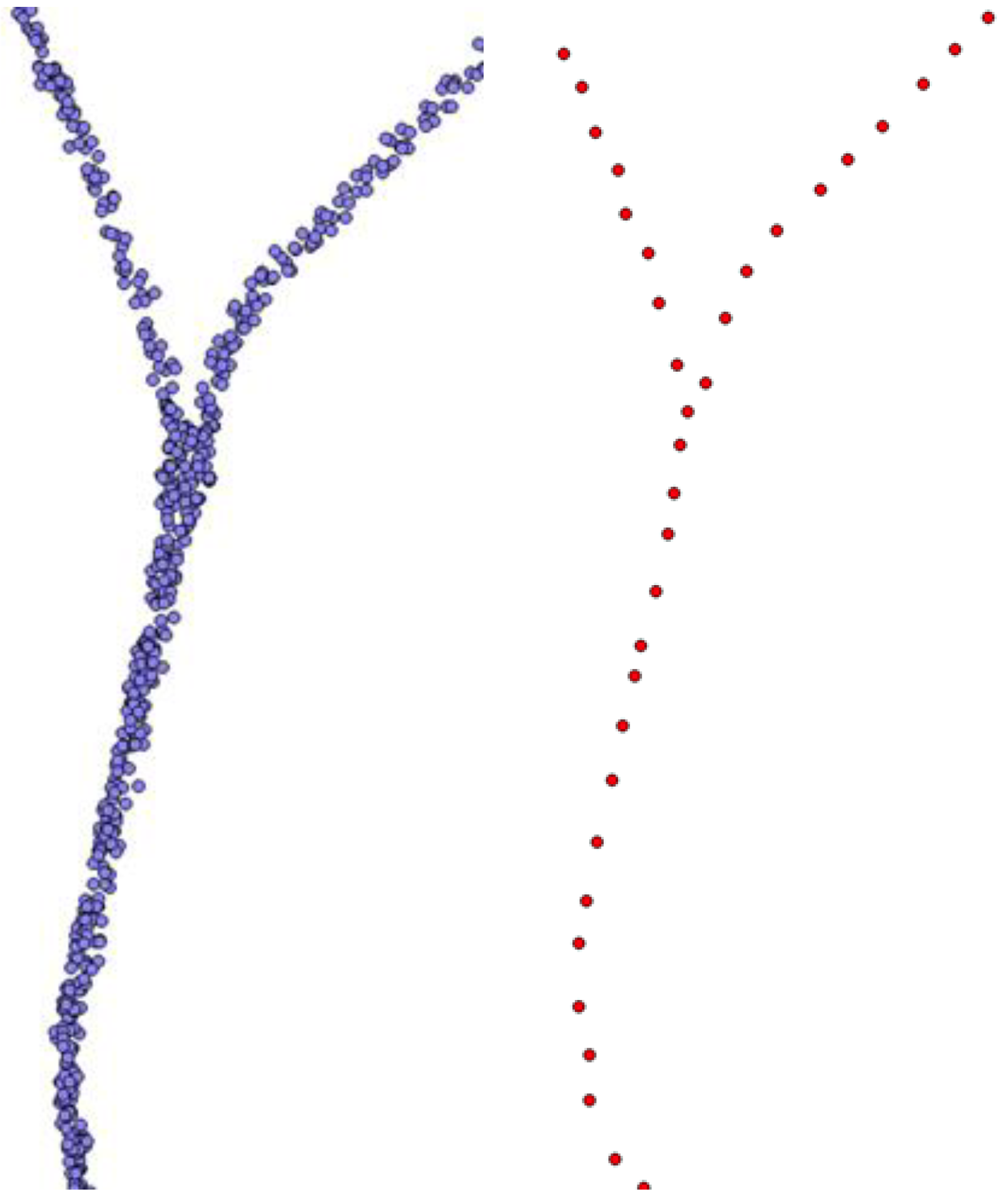
Figure 6 depicts a comparison of the GPS points in multiple trajectories and representative points extracted from this batch of GPS points. It can be seen that the algorithm greatly reduces the data redundancy with an almost uniform distribution of representative points while the shape of roads is preserved.
The update time t in the representative point attribute represents the timeliness of the point. By filtering out representative points that have not been updated for a given time, the accuracy and timeliness of the road network can be guaranteed.
3.3. Connecting Segment Extraction
Extracting representative points from the original trajectory data utilizes position information in the trajectory data. However, the extracted representative points lack the line segments to connect them, and it is impossible to obtain the road connectivity information from their respectively independent representative points. Therefore, it is also necessary to read the timing information in the original GPS trajectory and establish the connection relationship between the representative points.
By using the representative point extraction and update algorithm described in Section 3.2, the trajectory is converted into a set of representative point sequences. The order of the representative points in the sequences corresponds to the timing information in the original trajectory. Therefore, it is possible to use the connecting segment between two adjacent representative points to represent the road between these two representative points.
Definition 3.
Connecting segment. The Connecting segment refers to the line segment connecting two representative points, a and b, denoted as L = {a, b, n}, where n represents the number of occurrences of this connecting segment.
The connecting segment records the topological relationship between the representative points. By setting a threshold value for the number of occurrences of the connecting segment n and filtering out a part of the abnormal connecting segments with relatively few occurrences, the accuracy of the road network can be further improved. However, an excessively high threshold will filter out too many useful connecting segments and cause waste of trajectory data. Therefore, it is necessary to set reasonable values according to the number of input trajectories.
Algorithm 2 describes the process of extracting a connecting segment. Step 1–5 convert GPS points in the trajectory to representative points. Step 6 initializes a set which is used to save the connecting segments in the trajectory to be extracted. Step 7–10 split the trajectory into connecting segments and add them to the set. Finally, in Step 11, the extracted connecting segment set is returned.
| Algorithm 2 Connecting segment extraction algorithm |
|
3.4. Incremental Road Network Generation and Updating
The connecting segment represents the connectivity between the representative points which means there should be a road segment between the two connection points. However, the road conditions in real life are complex and varied. The distance between the two GPS points in the trajectory of the vehicle is different. If the road network is formed directly according to the time sequence of the trajectory, the situation in Figure 7 will occur, which is the connection manners of the representative points on the same road are various, and these connecting segments cannot accurately restore the shape of the actual road because of the longer length. Therefore, it is necessary to further optimize the connection method between the representative points to make them connected sequentially in the order of their locations and form a unique representation.
To find the real road network, a Delaunay triangulation network based on the representative points is created at first. Delaunay triangulation has the following excellent features [20,21]. (i) Uniqueness: No matter where it starts, the result will be consistent. (ii) Empty circle: There is no other point in the range of the circumcircle of any triangle. (iii) Maximum minimum angle: If the diagonals of a convex quadrilateral consisting of any two adjacent triangles are interchangeable, the minimum angle of the six internal angles will no longer increase after interchanging. Based on these three characters and the nature of real road network, almost all physically adjacent representative points along a road will be connected by edges of its Delaunay triangulation network as depicted in Figure 8.
After the Delaunay triangulation network is built, whenever a connecting segment is inputted, e.g., (p1, p5) in Figure 8, instead of adding (p1, p5) to the road network directly, a shortest path between p1 and p5 is searched in the Delaunay network and regarded as a real road segment, which is (p1, p2, p3, p4, p5) in this example. With this step, the various long length connecting segments are divided into multiple sequentially connected segments. The shortest path can be found with classical Dijkstra’s algorithm [22]. For the directed graph without negative weight, this is the fastest single-source-shortest-path algorithm known at present.
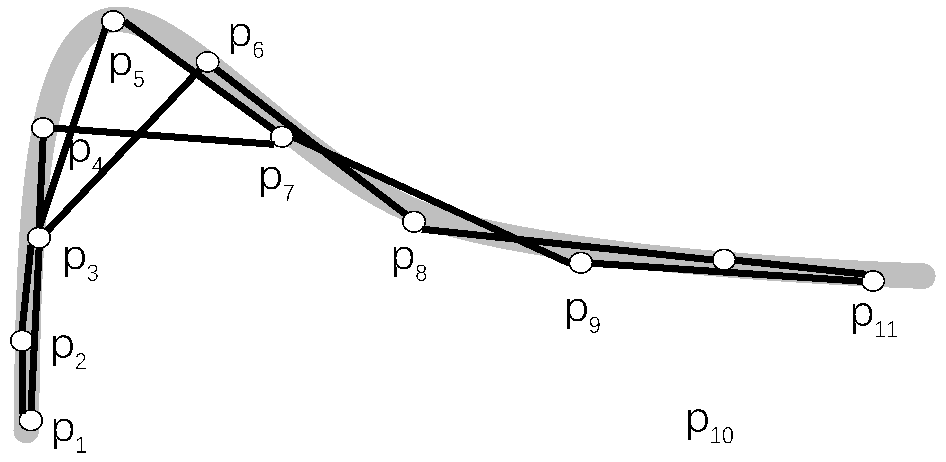
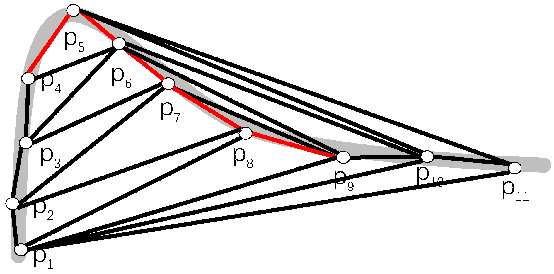
However, using the length of the Delaunay edge directly as the weight of Dijkstra’s algorithm will lead to the interpolation result at the curve not meeting expectations. As depicted in Figure 9, the red line segment in the figure is weighted by the length of the Delaunay edge, the Dijkstra algorithm is used to search for the shortest path from p4 to p7 and p7 to p9. Obviously, due to the neglect of p5 and p8, the resulting shape does not match the shape of the actual road. Generally, in the road generation process, we prefer multiple short lines to a direct long line.
Therefore, a new distance metric is designed as Equation (1). For all Delaunay triangulations, the weight of the Delaunay edge in the mesh is defined as the power of the length of the edge. The weight of Delaunay edge with endpoints a and b is calculated as:
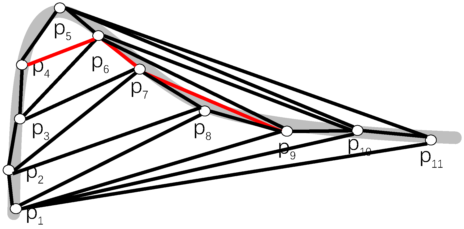
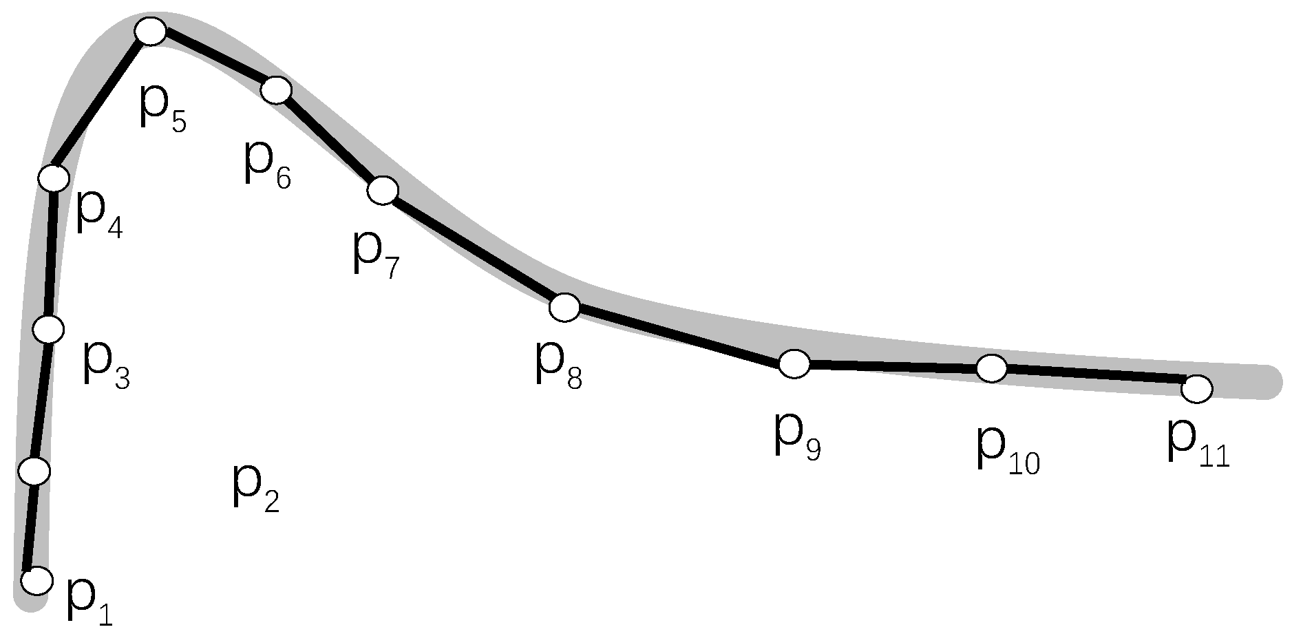
The parameter can be used to control the selection of the interpolation path. When is greater than 1, the path chosen by the algorithm will be biased towards those paths that contain more short segments. The larger is, the more obvious this trend is. Let , the Dijkstra algorithm is applied to search for the shortest path from p4 to p7 and p7 to p9. The result is depicted in the red line in Figure 10. Obviously, the red line segment’s shape conforms to the actual road shape. This result illustrates the feasibility of realizing the interpolation of the connecting segment at the bend by redefining the weight of the Delaunay edge.
According to the above interpolation algorithm, we interpolate all the connecting segments depicted in Figure 7 and get the road network graph as depicted in Figure 11. The representative points in Figure 11 are connected in order along the road. Each connecting segment is mapped to a Delaunay edge. Then, a figure with a height similar to the road shape is obtained.
The above algorithm implements the interpolation of the connecting segments based on the Delaunay triangulation constructed by the representative points. However, as the number of input vehicle trajectories increases, the number and position of the representative points will constantly change. The Delaunay triangulation formed by the representative points will also need to be changed. Benefiting from the regional nature of the Delaunay triangulation (adding, deleting or moving a vertex will only affect the adjacent triangle), when the representative point changes, its corresponding Delaunay triangulation only needs to be locally updated, which greatly reduces the computation time of the algorithm.
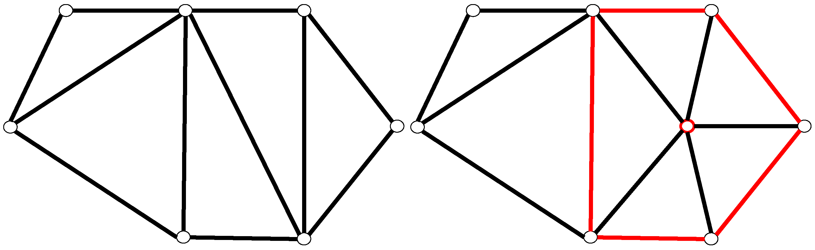
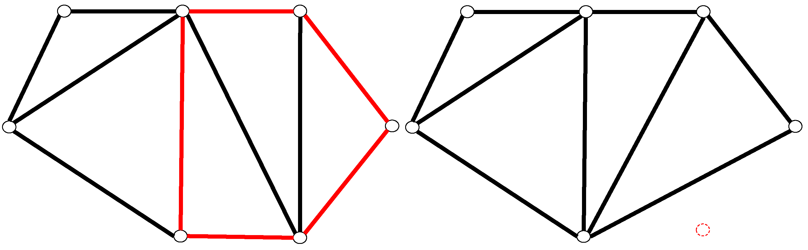
Figure 12 and Figure 13 depict the changes in the Delaunay triangulation caused by the addition and deletion of representative points, respectively [23,24]. Due to the regional of Delaunay triangulation, when adding/deleting a representative point causes the Delaunay triangulation to change, only the part of the connecting segment in the polygon whose structure changes is affected (marked with red line segments). Therefore, whenever the trajectory input changes the structure of the Delaunay triangulation, it is only necessary to re-interpolate the part of the connecting segment, together with the connecting segment extracted from the trajectory, to ensure that the road network through which this trajectory passes is properly updated. Note: The structural changes caused by the location update of the points in the Delaunay triangulation are essential point deletion and point addition processes, which are not discussed.
Algorithm 3 describes the process of road network generation and update. Step 4 determines whether the Delaunay triangulation exists in the first row. If not, Step 5–6 are executed. In Step 5, a Delaunay triangulation is constructed according to the input representative points, and, in Step 6, the Dijkstra algorithm is used to segment the connecting segments in the input trajectory and convert them into shorter Delaunay edges. If there is already a Delaunay triangulation built with representative points, the algorithm executes Step 8–10. In Step 8, the Delaunay triangulation is locally updated according to the newly added (updated) representative points, a new Delaunay triangulation and a set of connecting segments affected by the update triangulation are obtained. Then, in Step 9, the affected connecting segments are deleted from the original set of connecting segments. In Step 10, the new Delaunay triangulation is used to re-segment the affected connecting segments along with the connecting segments in the input trajectory. Finally, in Step 11, a Delaunay triangulation and a new set of connecting segments are returned.
| Algorithm 3 Road network generation and update algorithm |
|
Through the above steps, each connecting segment corresponds to a unique Delaunay edge, and each connecting segment is divided into more short line segments as many as possible while ensuring conformity with the road network. The generated road network graph has unique representative point connection method on the same road, and this connection method is closest to the actual road network shape. With the continuous input of vehicle trajectories, the generated shape of road network will become closer and closer to the actual road network.
4. Experimental Results and Analysis
Experimental platform: the experiment is performed on Intel Core I5-4440 CPU, 12GB memory, Windows 10 operating system, applying Python language to implement the above algorithms, QGIS as the trajectory display platform, and MySQL database to store trajectory data and other experimental data.
The experiment utilizes the all GPS trajectory data of all the trucks of a logistics company driving in Nanning during January 2015. The GPS point in the trajectory consists of the vehicle ID, time, position, and mileage. The sampling time interval of the GPS point is 10 s. A total number of 451,537 GPS points composed 5000 tracks.
Before conducting the experiment, the values of the three parameters and r need to be determined. Parameter (described in Section 3.4) is used to control the interpolation algorithm of the connecting segment in order to ensure that the road network formed at the curve is closer to the shape of the actual road. The larger is the , the more suitable is the interpolation algorithm for generating the graph with the larger corner angle. In practice, to ensure the normal traffic of all vehicles, the angle of the curve is usually not too large, so, in general, is enough to generate the correct road network graphics in most cases.
Parameter (described in Section 3.3) is applied to filter out some abnormal connecting segments in the road network. In general, the number of repeated abnormal connecting segments is much smaller than the normal connecting segments. Too high will cause some normal connecting segments to be filtered, resulting in waste of data. Therefore, the setting of depends on the quality of the input vehicle trajectory. If the preprocessed vehicle trajectory quality is high, the GPS points in the trajectory are evenly spaced and the corresponding GPS points are all on the normal road, then, a smaller can be set. Otherwise, a higher is required to filter abnormal line segments.
Parameter r (described in Section 3.2) corresponds to the representation range of the representative point, which generally depends on the road width and accuracy of the GPS device. According to the road width, parameter r should be at least larger than the widest road to cover every road and should be smaller than the smallest distance of any two adjacent roads to distinguish the two roads. According to the accuracy of the GPS device, parameter r should cover the largest distance error of the GPS. In our experiment data, we observed that the widest road is about 50 m and the distance between two adjacent roads are greater than 50 m in general. The GPS error is 10–50 m. Thus, we set m.
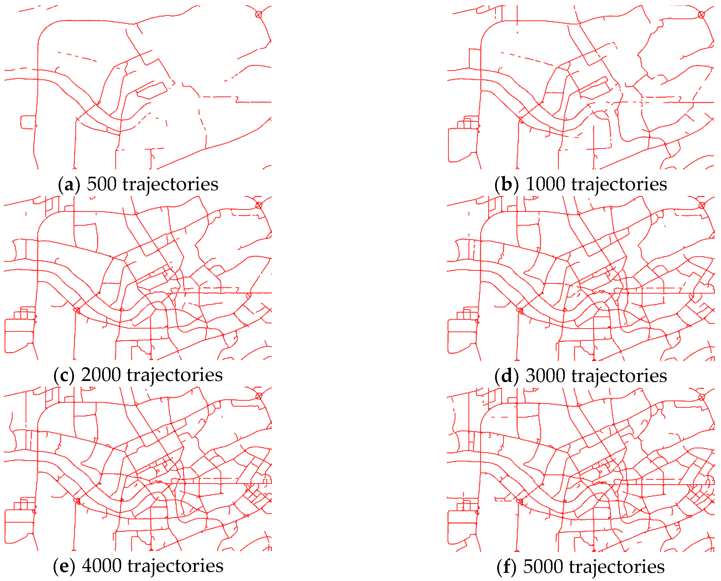
As discussed above, let , , , and the above trajectory data are inputted in turn, the generated road network graphics are intercepted as depicted in Figure 14 when the incremental algorithm proceeds to the 500th, 1000th, 2000th, 3000th, 4000th, and 5000th trajectory.
Comparing the graphs in Figure 14, it can be found that, with the continuous input of the vehicle trajectory, the generated road network becomes more and more complicated, and more and more details are presented. With a careful observation of each picture in Figure 14, it is found that there are many “breakpoints” in the road network generated at the beginning, which is because, when the number of trajectories is small, the number of repeated occurrences of some connecting segments is less than . However, it will be filtered when the road network is being generated and will not be displayed for the time being.
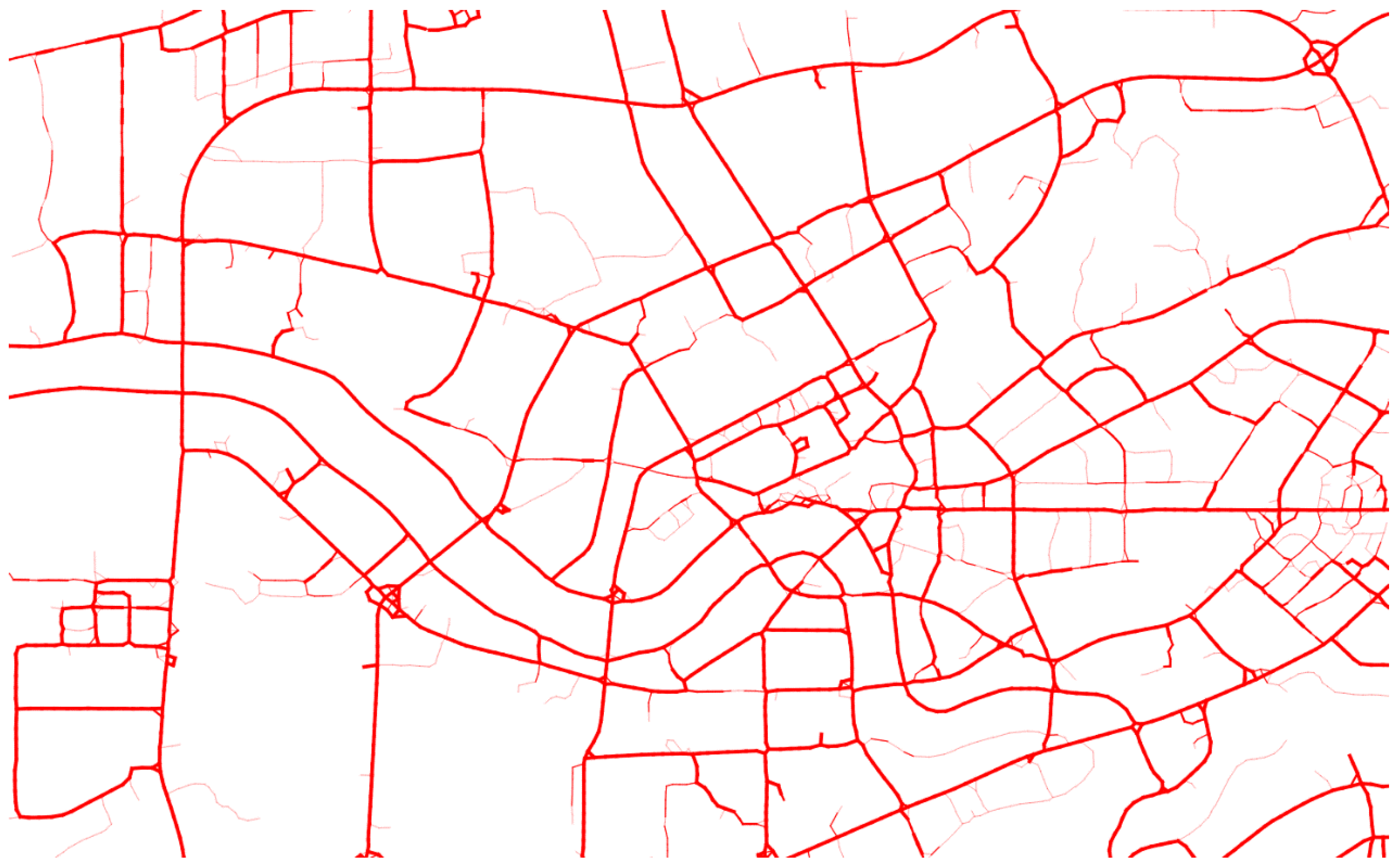
Fewer repeated occurrences of connecting segments does not mean those segments are abnormal. It may be because the number of vehicle trajectories corresponding to the road segment is small. However, in general, the more repeating the line segment is, the less likely it is an abnormal line segment. Therefore, according to the user’s accuracy requirements for the road network, the corresponding can be set. Figure 15 divides the number of repeated occurrences of the connecting segment by the thickness of the line segment, and divides the number of occurrences of the connecting segment into four steps according to 1–3 times, 4–6 times, 7–9 times, and ≥10 times, and draws from thin to coarse together on the same picture. In Figure 15, the influence of on the coverage of the generated road network can be visually seen. The higher is the , the higher is the accuracy of the obtained road network, while the smaller is the coverage range.
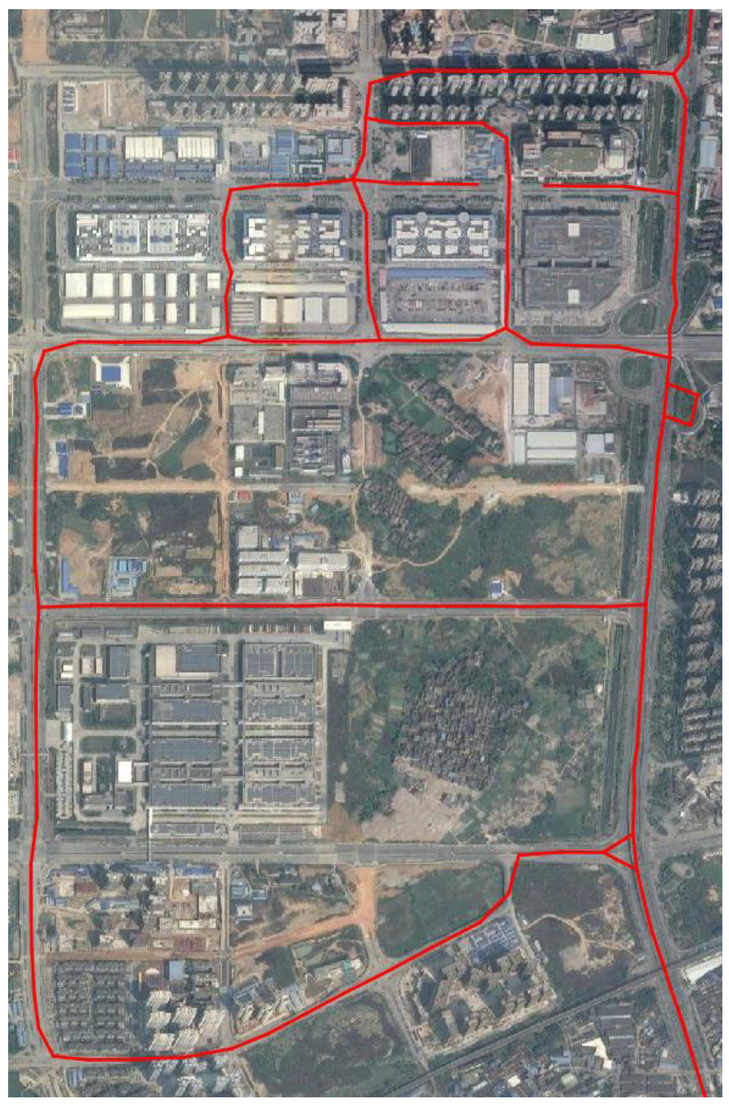
Figure 16 compares the generated road network graphics with the existing street map overlay. In Figure 16, the road network graph generated in this paper is consistent with the actual road network structure, and the line segment of the road network is located at the center of the road with high accuracy. However, some roads on the street map did not generate corresponding road network segments. This is because the experiment only applies the truck trajectories which cannot cover all roads in the area, thus, to generate a more complete road network, a variety of different vehicle trajectory data would be better. In addition, some road segments in the generated road network graphics do not have corresponding roads on the street map as depicted in Figure 16. By referring to the high-definition satellite map in Figure 17, it can be found that these segments have corresponding roads. However, the tradition road network update method is slower, so it has not been updated on the street map at the time of the experiments.
As the city continues to develop and expand, the city’s road information is constantly changing. After a new road in the city is constructed, there will be vehicles passing through this road to form a new trajectory. Through these trajectories, the algorithm can gradually “grow” the graph about this new road on the basis of the original road network.
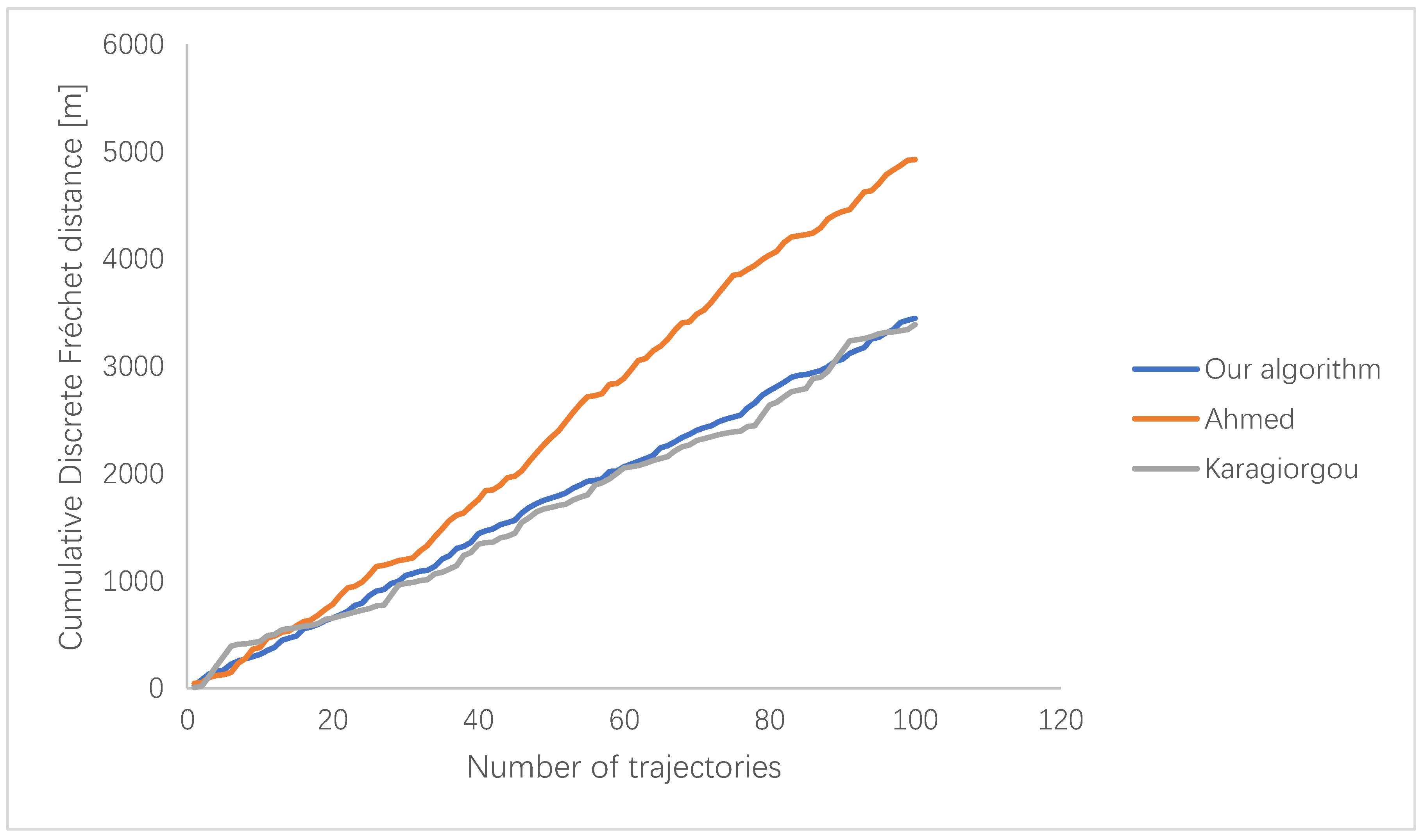
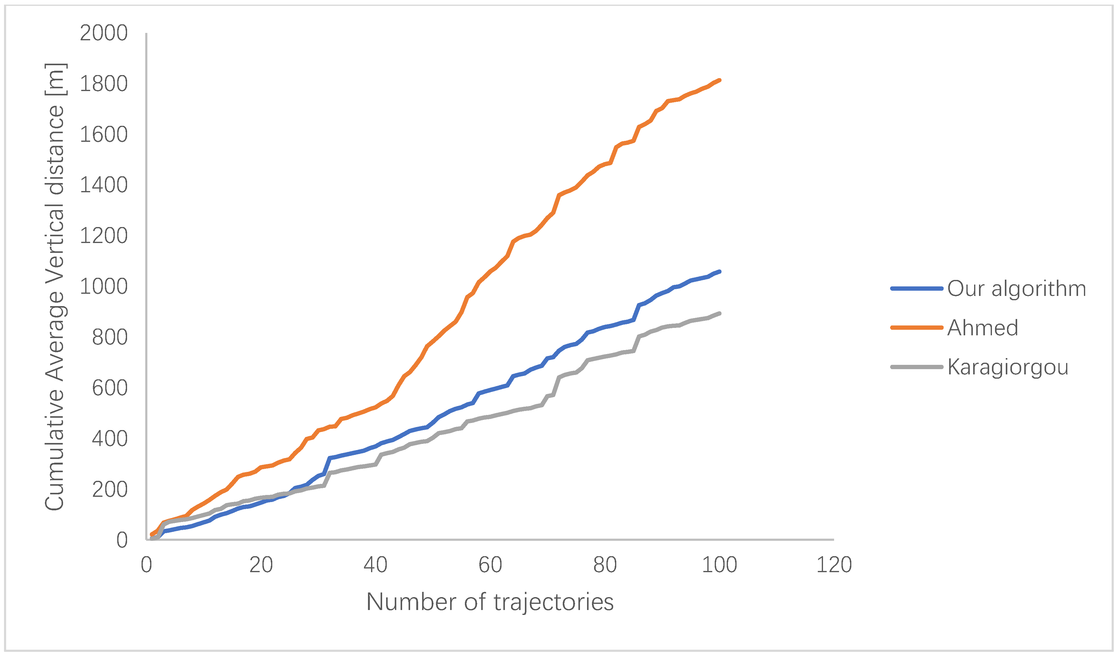
Karagiorgou et al. [16] used random sets of shortest paths to quantitatively measure the quality of the resulting road network. Their evaluation process can be summarized in three steps. In the first step, a ground-truth network is derived using the tracking data as a filter. The second step randomly selects the same set of origin and destination nodes and compute the respective shortest paths in ground-truth network and generated network. Finally, in step three, the Discrete Fréchet distance and the Average Vertical distance are used to compare the shortest paths. We used their method to quantitatively evaluate our algorithm and compared it to Ahmed’s [14] and Karagiorgou’s [16] algorithms, which have public realization on the Internet (https://github.com/pfoser/mapconstruction). Because our dataset has no ground truth, we chose Chicago dataset (provided by Biagioni and Eriksson [25,26], it contains 888 trajectories, and 119,360 GPS points) to compare the accuracy and speed of the three algorithms. We computed a set of 100 random shortest paths with origin and destination nodes uniformly distributed over the maps and compared the paths using the Discrete Fréchet distance and the Average Vertical distance measure. The results are shown in Figure 18 and Figure 19. We also list the execution time of these three algorithms in Table 1. Our algorithm has similar Discrete Fréchet distance but a little bigger Average Vertical distance compared to Karagiorgou’s algorithm which means Karagiorgou’s algorithm has higher accuracy. However, Karagiorgou’s algorithm is about 120 times slower than our method. Ahmed’s algorithm is a little bit faster than ours, as shown in Table 1, but its Discrete Fréchet distance and Average Vertical distance is much bigger than ours. We believe our algorithms has a better tradeoff between efficiency and accuracy.
5. Summary
This paper presents an algorithm for incrementally extracting road network graphics from vehicle trajectory data. Whether it is urban or extra-urban road, as long as there is corresponding vehicle trajectory data, the algorithm can be used to extract the road network. The generated road network has the advantages of timely updating (along with the change of actual traffic information) and high accuracy (the accuracy increases with the increase of the number of input trajectories). It greatly benefits the fields of intelligent transportation and car navigation. The algorithm proposed in this paper overcomes the shortcomings of long period and high cost of traditional road network generation methods. It can use vehicle trajectory data to generate road network at a lower cost and faster speed. The generated road network can change in time with the changes of road network (road repair, diversion, etc.), which is very important for route planning. In addition, the number of connecting segments not only shows its confidence, but also indicates the traffic volume of the section. More connecting segments means greater the traffic volume; this characteristic is also very helpful for urban traffic analysis. The innovations of this paper are as follows: (i) applying an incremental learning algorithm to record the effective information in the input trajectory data, thereby reducing the occupation of storage space and the time of calculation; and (ii) combining Dijkstra algorithm and Delaunay triangulation with the custom distance metric to realize the segmentation of the connecting segment, which makes the shape of the road network more in line with the actual road.
The experiments in this paper used the truck trajectory for testing and analysis. In addition to trucks, passenger car trajectories are also common and easy to collect trajectories. Compared to trucks, passenger cars can be found in residential areas or other narrow roads in addition to the urban main roads and highways. Therefore, the coverage of the passenger car trajectories is wider, and the formed road network is denser. Thus, using passenger car trajectories to generate road network requires higher accuracy of trajectory. We will find ways to get some passenger car trajectories for experiments in future work. Due to the lack of corresponding ground truth for the experimental data used in this paper, we were unable to verify the generated road network. In future work, we will try our best to find the corresponding ground truth to prove how incremental extraction helps improve the accuracy. The method in this paper does not distinguish the direction of vehicle trajectory, so, when there are two lanes in different directions on one road, the method cannot distinguish them. In the future work, we will focus on how to distinguish lanes in different directions and generate a road network with directions. The method described in this paper has certain discrepancies between the shape of the road network generated by the three-dimensional road sections with complicated road shapes such as overpasses and the actual road shape. The experimental parameters of this paper are only suitable for building a two-dimensional road network. Therefore, only the latitude and longitude properties of the vehicle are used and the altitude of the vehicle is discarded. In the future, we will focus on the extraction of the three-dimensional road network shape, and further enhance the application range of this method.
Author Contributions
Data curation and cleaning, B.S.; Methodology, Z.N. and L.X.; Software, Z.N.; Writing—original draft, Z.N.; Writing—review & editing, L.X. and T.X.; Project administration, L.X. and Y.Z.; Funding acquisition, L.X.
Funding
This research was funded by the General Program of National Natural Science Foundation of China, grant number 11772301, and the Project of Natural Science Foundation of Zhejiang Province, China, grant number LY17F020016.
Conflicts of Interest
The authors declare no conflicts of interest.
References
- Cao, L.; Krumm, J. From GPS traces to a routable road map. In Proceedings of the 17th ACM SIGSPATIAL International Conference on Advances in Geographic Information Systems, Seattle, WA, USA, 4–6 November 2009; pp. 3–12. [Google Scholar]
- Hu, J.; Razdan, A.; Femiani, J.C.; Cui, M.; Wonka, P. Road network extraction and intersection detection from aerial images by tracking road footprints. IEEE Trans. Geosci. Remote Sens. 2007, 45, 4144–4157. [Google Scholar] [CrossRef]
- Dal Poz, A.P.; Zanin, R.B.; do Vale, G.M. Automated extraction of road network from medium-and high-resolution images. Pattern Recognit. Image Anal. 2006, 16, 239–248. [Google Scholar] [CrossRef]
- Sghaier, M.O.; Lepage, R. Road extraction from very high resolution remote sensing optical images based on texture analysis and beamlet transform. IEEE J. Sel. Top. Appl. Earth Obs. Remote Sens. 2016, 9, 1946–1958. [Google Scholar] [CrossRef]
- Goodchild, M.F. Citizens as sensors: The world of volunteered geography. GeoJournal 2007, 69, 211–221. [Google Scholar] [CrossRef]
- Qiu, J.; Wang, R. Automatic extraction of road networks from GPS traces. Photogramm. Eng. Remote Sens. 2016, 82, 593–604. [Google Scholar] [CrossRef]
- Niu, Z.; Li, S.; Pousaeid, N. Road extraction using smart phones GPS. In Proceedings of the 2nd International Conference on Computing for Geospatial Research & Applications, Washington, DC, USA, 23–25 May 2011; p. 22. [Google Scholar]
- Li, H.; Kulik, L.; Ramamohanarao, K. Automatic generation and validation of road maps from GPS trajectory data sets. In Proceedings of the 25th ACM International on Conference on Information and Knowledge Management, Indianapolis, IN, USA, 24–28 October 2016; pp. 1523–1532. [Google Scholar]
- Edelkamp, S.; Schrödl, S. Route planning and map inference with global positioning traces. In Computer Science in Perspective; Klein, R., Six, H.-W., Wegner, L., Eds.; Springer: Berlin/Heidelberg, Germany, 2003; pp. 128–151. [Google Scholar]
- Chen, C.; Cheng, Y. Roads digital map generation with multi-track GPS data. In Proceedings of the IEEE International Workshop on Education Technology and Training, 2008 and 2008 International Workshop on Geoscience and Remote Sensing, ETT and GRS 2008, Shanghai, China, 21–22 December 2008; Volume 1, pp. 508–511. [Google Scholar]
- Chen, D.; Guibas, L.J.; Hershberger, J.; Sun, J. Road network reconstruction for organizing paths. In Proceedings of the Twenty-First Annual ACM-SIAM Symposium on Discrete Algorithms, Austin, TX, USA, 17–19 January 2010; Charikar, M., Ed.; Society for Industrial and Applied Mathematics: Philadelphia, PA, USA, 2010; pp. 1309–1320. [Google Scholar]
- Zhang, L.; Thiemann, F.; Sester, M. Integration of GPS traces with road map. In Proceedings of the ACM Third International Workshop on Computational Transportation Science, San Jose, CA, USA, 2 November 2010; pp. 17–22. [Google Scholar]
- Bruntrup, R.; Edelkamp, S.; Jabbar, S.; Scholz, B. Incremental map generation with GPS traces. In Proceedings of the IEEE Intelligent Transportation Systems, Vienna, Austria, 16 September 2005; pp. 574–579. [Google Scholar]
- Ahmed, M.; Wenk, C. Constructing street networks from GPS trajectories. In European Symposium on Algorithms, Proceedings of the 20th Annual European Conference on Algorithms, Ljubljana, Slovenia, 10–12 September 2012; Springer: Berlin/Heidelberg, Germany, 2012; pp. 60–71. [Google Scholar]
- Fathi, A.; Krumm, J. Detecting road intersections from GPS traces. In Geographic Information Science, Proceedings of the 6th International Conference on Geographic Information Science, Zurich, Switzerland, 14–17 September 2010; Fabrikant, S.I., Reichenbacher, T., van Kreveld, M., Schlieder, C., Eds.; Springer: Berlin/Heidelberg, Germany, 2010; pp. 56–69. [Google Scholar]
- Karagiorgou, S.; Pfoser, D. On vehicle tracking data-based road network generation. In Proceedings of the ACM 20th International Conference on Advances in Geographic Information Systems, Redondo Beach, CA, USA, 6–9 November 2012; pp. 89–98. [Google Scholar]
- Xu, J.J.; Zheng, K.; Chi, M.M.; Zhu, Y.Y.; Yu, X.H.; Zhou, X.F. Trajectory big data: Data, applications and techniques. J. Commun. 2015, 36, 97–105. (In Chinese) [Google Scholar]
- Gao, Q.; Zhang, F.L.; Wang, R.J.; Zhou, F. Trajectory big data: A review of key technologies in data processing. RuanJian Xue Bao. J. Softw. 2017, 28, 959–992. (In Chinese) [Google Scholar]
- Zheng, Y.; Zhou, X. (Eds.) Computing with Spatial Trajectories; Springer Science & Business Media: Berlin, Germany, 2011. [Google Scholar]
- Ekpenyong, F.; Palmer-Brown, D.; Brimicombe, A. Extracting road information from recorded GPS data using snap-drift neural network. Neurocomputing 2009, 73, 24–36. [Google Scholar] [CrossRef]
- Lee, D.T.; Schachter, B.J. Two algorithms for constructing a Delaunay triangulation. Int. J. Comput. Inf. Sci. 1980, 9, 219–242. [Google Scholar] [CrossRef]
- Cormen, T.H.; Leiserson, C.E.; Rivest, R.L.; Stein, C. Introduction to Algorithms, 2nd ed.; The Massachusetts Institute of Technology: Cambridge, MA, USA, 2001. [Google Scholar]
- Watson, D.F. Computing the n-dimensional Delaunay tessellation with application to Voronoi polytopes. Comput. J. 1981, 24, 167–172. [Google Scholar] [CrossRef] [Green Version]
- Mostafavi, M.A.; Gold, C.; Dakowicz, M. Delete and insert operations in Voronoi/Delaunay methods and applications. Comput. Geosci. 2003, 29, 523–530. [Google Scholar] [CrossRef]
- Biagioni, J.; Eriksson, J. Inferring road maps from global positioning system traces: Survey and comparative evaluation. Transport. Res. Rec. 2012, 2291, 61–71. [Google Scholar] [CrossRef]
- Biagioni, J.; Eriksson, J. Map inference in the face of noise and disparity. In Proceedings of the ACM 20th International Conference on Advances in Geographic Information Systems, Redondo Beach, CA, USA, 6–9 November 2012; pp. 79–88. [Google Scholar]
Figure 1.
Vehicle trajectories during a certain period of a certain area.

Figure 2.
Road network extraction algorithm flow.

Figure 3.
Missing points in the trajectory.

Figure 4.
Noise points in the trajectory.

Figure 5.
Stationary points in the trajectory.

Figure 6.
Comparison of original GPS points (left) and representative points (right).

Figure 7.
Connect the graphics formed by the representative points according to the track timing.

Figure 8.
Constructing Delaunay Triangulation with representative points.

Figure 9.
Interpolation results with edges as the weight (Red line segment).

Figure 10.
Interpolation result with the weight of the power () of the edge length.

Figure 11.
Interpolation results for all connecting segments.

Figure 12.
Insert a point in Delaunay Triangulation Network.

Figure 13.
Delete a point of Delaunay Triangulation Network.

Figure 14.
Road networks generated by different numbers of trajectories.

Figure 15.
Using line segment thickness to distinguish the number of occurrences of connecting segments.
Figure 15.
Using line segment thickness to distinguish the number of occurrences of connecting segments.

Figure 16.
Comparison between road network and street map.

Figure 17.
Comparison between road network and high-definition satellite map ().

Figure 18.
Cumulative Discrete Fréchet distance.

Figure 19.
Cumulative Average Vertical distance.


Table 1.
Execution time.
| Algorithm Name | Time |
|---|---|
| Our algorithm | 6 min 5 s |
| Ahmed | 4 min 35 s |
| Karagiorgou | 745 min |
© 2018 by the authors. Licensee MDPI, Basel, Switzerland. This article is an open access article distributed under the terms and conditions of the Creative Commons Attribution (CC BY) license (http://creativecommons.org/licenses/by/4.0/).
Share and Cite
MDPI and ACS Style
Ni, Z.; Xie, L.; Xie, T.; Shi, B.; Zheng, Y. Incremental Road Network Generation Based on Vehicle Trajectories. ISPRS Int. J. Geo-Inf. 2018, 7, 382. https://doi.org/10.3390/ijgi7100382
AMA Style
Ni Z, Xie L, Xie T, Shi B, Zheng Y. Incremental Road Network Generation Based on Vehicle Trajectories. ISPRS International Journal of Geo-Information. 2018; 7(10):382. https://doi.org/10.3390/ijgi7100382
Chicago/Turabian StyleNi, Zhongyi, Lijun Xie, Tian Xie, Binhua Shi, and Yao Zheng. 2018. "Incremental Road Network Generation Based on Vehicle Trajectories" ISPRS International Journal of Geo-Information 7, no. 10: 382. https://doi.org/10.3390/ijgi7100382
Note that from the first issue of 2016, this journal uses article numbers instead of page numbers. See further details here.