Comparison of Split Window Algorithms for Retrieving Measurements of Sea Surface Temperature from MODIS Data in Near-Land Coastal Waters


Research Institute for Geo-Hydrological Protection (IRPI), National Research Council (CNR), Perugia 06128, Italy
ISPRS Int. J. Geo-Inf. 2018, 7(1), 30; https://doi.org/10.3390/ijgi7010030
Submission received: 10 November 2017
/
Revised: 9 January 2018
/
Accepted: 12 January 2018
/
Published: 18 January 2018
Abstract
:Split window (SW) methods, which have been successfully used to retrieve measurements of land surface temperature (LST) and sea surface temperature (SST) from MODIS images, were exploited to evaluate the SST data of three sections of Italian coastal waters. For this purpose, sea surface emissivity (SSE) values were estimated by adding the effects of salinity and total suspended particulate matter (SPM) concentrations, sea surface wind speed, and zenith observation angle. The total column atmospheric water vapor contents were retrieved from MODIS data. SST data retrieved from MODIS images using these algorithms were compared with SSTskin measurements evaluated from in situ data. The comparison showed that the algorithms for retrieving LST measurements minimized the error in SST data in near-land coastal waters with respect to the algorithms for retrieving SST measurements: a method for retrieving LST measurements highlighted the smallest root-mean-square deviation (RMSD) value (0.48 K) and values of maximum bias and standard deviation (σ) equal to −3.45 K and 0.41 K; the current operation algorithm for retrieving LST data highlighted the smallest values of maximum bias and σ (−1.37 K and 0.35 K) and an RMSD value of 0.66 K; and the current operation algorithm for retrieving global measurements of SST showed values of RMSD, maximum bias, and σ equal to 0.68 K, −1.90 K, and 0.40 K, respectively.
1. Introduction
Sea surface temperature (SST) plays a key role in life and processes in coastal waters [1,2,3,4,5,6,7,8,9,10,11,12]. Monitoring water quality is one of the most pressing requirements for ensuring the sustainability of these valuable and vulnerable habitats [2]. Nowadays, SST measurements of coastal waters retrieved from remote images have a wide variety of applications such as: the analysis of temperature influence over benthic organisms [1,3]; the assessment of potential aquaculture sites [4]; the detection of ground water discharge [5]; the hydrographic characterization of nearshore waters [6]; the monitoring of river plumes [7], thermal plume contaminations [8], and upwelling phenomena [9]; quantifying complex thermal environments on coral reefs [10,11]; and the study of the interactions between residual circulation, tidal mixing, and fresh influence [12]. Many of these applications have stringent accuracy requirements [1,3,4,8,9,10,11,12].
Nevertheless, errors in SST measurements retrieved from remote images have been reported by several papers [1,3,8,9,10,11]. Moreover, the differences between the in situ and satellite measurements of coastal sea temperature have also been evaluated by other authors [13,14,15], where this error can be as large as 6 °C [15]. All of these papers specifically analyzed SST data retrieved from advanced very high–resolution radiometer (AVHRR) and/or moderate resolution imaging spectroradiometer (MODIS) images using the operation split window (SW) algorithms [1,3,8,9,10,13,14,15]. Several factors can lead to errors in the SST data of near-land coastal waters retrieved from AVHRR and MODIS data with the operational algorithms for retrieving global SST data. The main factor is atmospheric correction, as it was developed for oceanographic applications [16,17,18]. The variations in total column atmospheric water vapor (W) content and in sea surface emissivity (SSE) values are considered negligible for retrieving global SST measurements [16,17,18,19].
The SSE value, in the thermal infrared region, is a function of total suspended particulate matter (SPM) and salinity concentrations, and the zenith observation angle, and is affected by sea surface roughness, which is a function of sea surface wind speed [20,21,22,23,24,25,26,27,28,29,30,31,32,33]. Therefore, not only the variations in W content and SSE value, but also in salinity and SPM concentrations, and sea surface wind speed, are considered negligible for retrieving global SST measurements by the operational SW algorithms of AVHRR and MODIS data, whereas the variability is a very important feature of coastal waters [34].
Moreover, the sea temperature of the pixels close to the coastal line along the scan direction is “mixed” with the land temperature [35], and the retrieving of land surface temperature (LST) measurements from satellite data takes into consideration the variations in land surface emissivity (LSE) and W values [36,37,38,39].
A variety of other SW methods were developed to optimize SST measurements such as the water vapor sea surface temperature algorithm, which includes W content as proposed by Emery et al. [40]; and the method proposed by Niclòs et al. [41], which also incorporates the SSE value, as authors considered the variation in SSE value comparable to the variation in emissivity of other land surfaces.
The paper compares the SST measurements retrieved from MODIS images with SW algorithms to identify the technique which minimizes the errors in SST data of near-land coastal waters. For this purpose, some SW techniques, which have been extensively tested and their coefficients retrieved from a robust dataset, were chosen from the algorithms for retrieving LST and SST measurements from MODIS images [16,17,18,37,38,39,41]. Their results were compared with the SSTskin values, which were estimated from in situ data. The SSE values included in the SW algorithms were estimated with the effects of salinity and SPM concentrations, sea surface wind speed, and zenith observation angle. The results highlighted that the best SW methods were the algorithms for retrieving LST data, which included the W and SSE values.
2. Materials
2.1. Study Area
The study area comprised three sections of Italian coastal waters (Figure 1a): the Manfredonia Gulf, Taranto Gulf, and the area close to Lesina Lagoon [42].
The Gulf of Manfredonia is a large and shallow gulf located in the western part of the southern Adriatic Sea (Figure 1a–c). The Gargano Promontory, i.e., the most prominent coastal bulge of the entire Adriatic, forms the northern border of the gulf and the estuary of the Ofanto River forms its southern border (Figure 1b). The gulf is named after the town of Manfredonia. The seafloor morphology is characterized by the significant increase in bathymetric gradient from the 30 m isobath to the coastline (Figure 1c), which is due to the sediment transported by the north Adriatic current [43]. The literature indicates that the coastal marine ecosystems of the Manfredonia Gulf are influenced by agricultural, industrial, and urban activities [44,45]. Fifteen measurement locations, situated at a distance of about 4 km from the coastline and between bathymetric lines of 10 and 15 m, were selected for describing these waters (Figure 1b,c). Sampling at these locations was carried out over four days and some were monitored several times. Each water column was characterized by features completely different from features of other water columns that were monitored in the same position during different days. In total, 39 different water columns were analyzed and, among these, 31 locations were observed within ±2 h with respect to MODIS overpasses [13].
The Taranto Gulf is a large square shaped gulf, i.e., 140 by 140 km, which is located in the northwestern part of the Ionian Sea (Figure 1a,d,e). The gulf is named after the town of Taranto. The seafloor morphology is characterized by the Taranto Valley, i.e., the foreland basin of the southern Italian orogenic, which crosses the Gulf of Taranto from the northwest to southeast [46]. The coastal marine ecosystems have been altered by iron and steel factories (i.e., Ilva is the most important steel production plant in Europe), petroleum refineries, and the intensive maritime traffic [47,48]. Since their environment impacts are great, the Taranto province was officially classified as an “Area of High Environmental Risk” by the national government (Italian Law n. 349/1986), and later included in the 14 “Sites of National Interest” (Italian Law n. 426/1998). The environmental remediation of this site has been identified as a national priority (Ministerial Decree n. 468/2002). Seven measurement locations situated at different distances from the coastline (i.e., from 2 to 12 km) and at different depths (i.e., from 23 to 303 m) were chosen to analyze these waters (Figure 1d,e). All these locations were monitored three times over four days and each water column was characterized by features completely different from features of other water columns which were monitored in the same position during different days. In total, 21 different water columns were analyzed and of these, 19 locations were observed within ±2 h with respect to MODIS overpasses [13].
Coastal waters close to Lesina Lagoon are situated north of the promontory of Gargano in the western part of the southern Adriatic Sea (Figure 1a,f,g). The seafloor morphology is characterized by the progressive increase of the forest dip in this coastal area. Cattaneo et al. [49] argued that the Gargano Promontory, which is very prominent toward the Adriatic Sea, acts as an obstacle to a sediment dispersal system as it changes the direction and velocity of the western Adriatic coastal current. Lesina Lagoon is situated north of the promontory of Gargano (Figure 1f,g) and is about 22 km long, with a total area of about 51 km2. The lagoon is characterized by shallow water, i.e., from 0.75 to 1.5 m, and a limited sea-lagoon exchange. Human intervention in the Lesina Lagoon such as an accumulation shelf of nutrients, introduction of opportunistic species, protection of sea-lagoon exchange, and commercial activities of fishing and aquaculture, has influenced the quality of coastal and lagoon environments [50]. Six measurement locations situated at distance of about 10 km from the coastline and around a bathymetric line of 20 m were selected for describing the waters close to Lesina Lagoon (Figure 1f,g). Six observations were monitored within ±2 h with respect to the MODIS overpass [13].
2.2. In Situ and Satellite Data
A cruise undertaken to characterize these coastal areas was carried out aboard the ship Dallaporta, which belongs to the Italian National Research Council (CNR) [42]. The location of each measurement observation was chosen in accordance with Mueller et al. [34] as per the protocol and knowledge of these areas of study. Sea temperature measurements of each water column were acquired with three multi-parametric platforms [13]. Data were processed in accordance with UNESCO standards [51].
Since the infrared radiometer on board the satellite acquires the brightness temperature at the surface skin layer of the water column (SSTskin), the measurements of sea temperature acquired with the three multi-parametric platforms were exploited to evaluate the SSTskin values. For this purpose, the model for retrieving diurnal SSTskin data (which was proposed by Webster et al. [52]) was applied (Table 1) and the resultant values of SSTskin were validated using values obtained with a model for retrieving diurnal SSTskin measurements (as proposed by Fairall et al. [53]). These diurnal methods were selected as they were extensively tested with in situ measurements under light-to-moderate wind conditions and have been confirmed by several authors [54,55,56,57].
Water samples collected at each location were analyzed in the laboratory to calculate the SPM concentration in accordance with the protocols laid down Mueller et al. [58] and Pegau et al. [59]. All observed waters were classified as coastal waters in accordance with the protocol described by Mueller et al. [34], as their concentrations of SPM were more than 0.5 mg/L (Table 1).
Nine images from the MODIS sensor on board the Aqua satellite were acquired under clear sky conditions during the oceanographic cruise (Table 1). The MODIS data (i.e., MODIS Level 1B data set, MYD021KM, which contains calibrated and geolocated radiances at-aperture for all 36 MODIS spectral bands at 1km resolution) were obtained from NASA’s Distributed Active Archive Centers.
3. Methods
3.1. Operational Algorithms for Retrieving Global Data of Sea Surface Temperature (SST) from Moderate Resolution Imaging Spectroradiometer (MODIS) Data
Brown et al. [16] introduced the first operational algorithm for retrieving SST measurements of from MODIS bands 31 and 32, which has the following form:
where T31 and T32 are the brightness temperature at satellite level of MODIS bands 31 and 32 in °C, respectively; Tsfc is an estimate of surface temperature in °C; θ is the satellite zenith angle; and c1, c2, c3, and c4 are constant coefficients. The authors [16] provided two distinct sets of coefficients: one was retrieved from a global dataset of 1200 quality controlled radiosondes, and another was derived from European Center Medium Weather Forecast (ECMWF) assimilation model marine atmospheres.
Collection 5 introduced new coefficients of the operational algorithm (Equation (1)), which were estimated for each month of any year from training data collected in 2004 [18]. Throughout this paper, SST measurements (named SST1(radiosonde based), SST1(ECMWF based), and SST1(collection 5)) were used to identify the data obtained with Equation (1) using the coefficients derived from radiosondes and the ECMWF assimilation model, and the coefficients of collection 5, respectively.
Collection 6, which was proposed by Kilpatrick et al. [17], introduced new coefficients and added three correction terms to the operation algorithm, i.e., a term related to the mirror side correction (mirror-side) and two terms related to zenith angle correction (θ). SST measurements were obtained with the following equation:
The coefficients of collection 6 were estimated using a generalized linear model, which was run multiple times to create 72 sets of coefficients corresponding to 12 months multiplied by six latitude bands [17]. Throughout this paper, SST measurements obtained using the coefficients and the method proposed by [17] were identified as SST2(collection 6) data.
3.2. Algorithms for Retrieving SST Data from MODIS Data
The MODIS team developed and modified only not-linear SW algorithms for retrieving SST measurements from MODIS data [60], whereas Sobrino et al. [37] proposed two linear SW algorithms and a linear quadratic SW technique for retrieving SST data from MODIS bands 31 and 32. Moreover, Sobrino et al. [37] introduced two terms which depend on the W value in a linear SW method. The algorithms assume the following forms:
where T31 and T32 are the brightness temperature at satellite level of MODIS bands 31 and 32 in K, respectively; W is the total amount of the atmospheric water vapor content in g/cm2; and a0, a1, a2, and a3 are the coefficients estimated from a set of 61 radiosonde observations and tested from a different set of 183 radiosonde observations. Therefore, the authors simulated MODIS data with the MODerate resolution atmospheric TRANsmission (MODTRAN) radiative transfer program and estimated a total error using both set radiosonde observations [37]. Throughout this paper, the SST measurements estimated with Equations (3)–(5) were identified as SST3, SST4, and SST5 data.
Niclòs et al. [41] considered not only the W content, but also the SSE value as fundamental variables to retrieve accurate SST measurements, and incorporated separate terms for W and SSE. The algorithm assumes the following form:
where T31 and T32 are the brightness temperature at satellite level of MODIS bands 31 and 32 in K, respectively; W is total atmospheric water vapor content in g/cm2; SSE31 and SSE32 are the sea surface emissivity of MODIS bands 31 and 32, respectively; and a1, a2, b1, b2, c1, c2, α0, α1, α2, β0, β1, and β2 are constant coefficients provided by [41]. The SAFREE radio-sounding database was exploited to develop the algorithm [61]. The SST measurements retrieved from the MODIS images were validated with in situ data [41]. Throughout this paper, the SST measurements obtained using method the proposed by [41] were identified as SST6 data.
3.3. Current Operational Algorithm for Retrieving Land Surface Temperature (LST) Data from MODIS Data
The authors of the current operational method for retrieving LST measurements [39] proposed estimating the LST values with a generalized SW algorithm [38], if the LSE values are known. Therefore, the LST measurements were evaluated with the following equation:
where T31 and T32 are the brightness temperature at satellite level of MODIS bands 31 and 32 in K, respectively; LSE31 and LSE32 are land surface emissivity of MODIS bands 31 and 32, respectively; A1, A2, A3, B1, B2, B3, and C are the coefficients which depend on column water vapor (cm), surface air temperature (K), and zenith observation angle values [38]. Throughout this paper, the LST measurements obtained using the method proposed by Wan and Dozier [38] were identified as LST1 data.
3.4. Algorithms for Retrieving LST Data from MODIS Data
Sobrino et al. [37] also proposed three models for estimating LST measurements using MODIS bands 31 and 32. The LST measurements are given by the following three equations:
where T31 and T32 are the brightness temperature at satellite level of MODIS bands 31 and 32 in K, respectively; W is the total atmospheric water vapor content in g/cm2; LSE31 and LSE32 are land surface emissivity of MODIS bands 31 and 32, respectively; and a1 to a14 are constant coefficients. As above-mentioned, the authors obtained the coefficients of these algorithms through 61 radiosonde observations, tested the methods with 183 radiosonde observations, and simulated MODIS data with the MODTRAN radiative transfer program. Therefore, they estimated error using both sets of radiosonde observations, and compared the retrieved values of LST with in situ measurements [37]. Throughout this paper, the LST measurements obtained using the method proposed by [37] with Equations (8)–(10) were identified as LST2, LST3, and LST4 data, respectively.
3.5. Estimation of Input Data
Since the brightness temperatures in MODIS bands 31 and 32 and zenith observation angles were derived from MODIS data, the SSE values in MODIS bands 31 and 32 and the W contents are required to retrieve SST measurements from MODIS images using the Equations (4), (6), and (8)–(10).
As above-mentioned, the variation in SSE value is due to the variation in salinity (S) and SPM concentrations, and in sea surface wind speed (U) and zenith observation angle (θ); the previous papers have evaluated these four effects on SSE values [20,21,22,23,24,25,26,27,28,29,30,31,32,33].
For this purpose, the emissivity values of the pure water in MODIS bands 31 and 32 were calculated by the model described by Masuda et al. [23], as these values have been confirmed by several authors [24,28,29,30,33].
The effect of S concentration on SSE values in MODIS bands 31 and 32 was obtained by the Newman et al. [25] model. This model was chosen because the authors investigated SSE behavior with respect to the salinity concentration using in situ data and their results, in this spectral region, were confirmed by SSE values of the most adopted model [21]. Therefore, the S effect on SSE values in MODIS bands 31 and 32 of these coastal waters was estimated from measured concentrations of salinity.
Wen-Yao et al. [31] and Wei et al. [32] retrieved SSE behaviors with respect to SPM concentrations from measurements of thermal radiometers at 8–14 μm in the laboratory. They agreed that the SSE value decreased with an increase in the SPM concentrations that were included in the water samples [31,32]. Therefore, the SPM effect on SSE values in MODIS bands 31 and 32 of these coastal waters was estimated from in situ data using the equation proposed by [31].
Since MODIS acquisitions over all stations on 14 August 2011 were performed with zenith observation angles greater than 50°, and the SSE values tabulated with these angles by the Masuda et al. [23] model have not been confirmed by some authors [22,26,27,30], the effects of U and θ on SSE values in MODIS bands 31 and 32 were obtained with the equations proposed by Niclòs and Caselles [26]. Therefore, these values were retrieved from sea surface wind speeds measured during the cruise and the zenith observation angle of MODIS data. The results were validated with SSE data calculated by Masuda et al. [23]. The root-mean-square deviation (RMSD) values between the resultant data in MODIS bands 31 and 32 and SSE values calculated with the model in [23] were equal to 0.008 and 0.009, respectively. In accordance with the previous papers [22,26,27,30] that did not confirm the SSE values tabulated with angles greater than 50° by Masuda et al. [23], the RMSD values of MODIS bands 31 and 32 acquired on 14 August 2011 were the greatest, i.e., 0.020 and 0.017, respectively.
4. Results and Discussion
SSTskin data were compared with SST1(radiosonde based), SST1(ECMWF based), SST1(collection 5), and SST2(collection 6) measurements retrieved from MODIS bands 31 and 32 with the operational algorithms for retrieving the global data of SST proposed by [16,17,18] (Table 2).
The SSTskin data were compared with the SST3, SST4, SST5, and SST6 measurements retrieved from MODIS bands 31 and 32 with the algorithms for retrieving SST data proposed by Sobrino et al. [37] and Niclòs et al. [41] (Table 3).
The SSTskin data were compared the LST1, LST2, LST3, and LST4 measurements retrieved from MODIS bands 31 and 32 with the current operation algorithm for retrieving LST measurements [38] and with the three algorithms for retrieving LST measurements proposed by [37] (Table 4).
The analysis of error in SST1(radiosonde based), SST1(ECMWF based), SST1(collection 5), SST2(collection 6), SST3, SST4, SST5, SST6, LST1, LST2, LST3, and LST4 measurements showed that the biases were both warm and cold. The bias is, specifically, equal to the SST data retrieved from satellite images minus the ones measured in situ. The biases in the SST1(radiosonde based) and SST1(ECMWF based) measurements were cold in all monitored locations. The biases in the LST4 measurements were warm, except for the data of the locations monitored on 12 and 14 August 2011. Therefore, the SST1(radiosonde based) and SST1(ECMWF based) measurements always underestimated the SST data of these coastal waters, and the LST4 measurements overestimated these data. The other data of SST showed both warm and cold biases in the locations monitored during the same day. The RMDS values were exploited to identify the methods which minimized the error in SST measurements in these coastal waters.
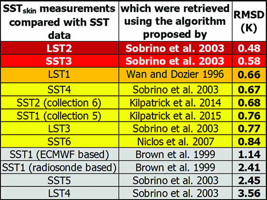
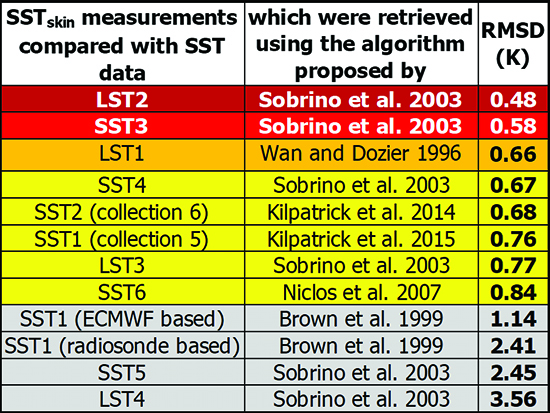
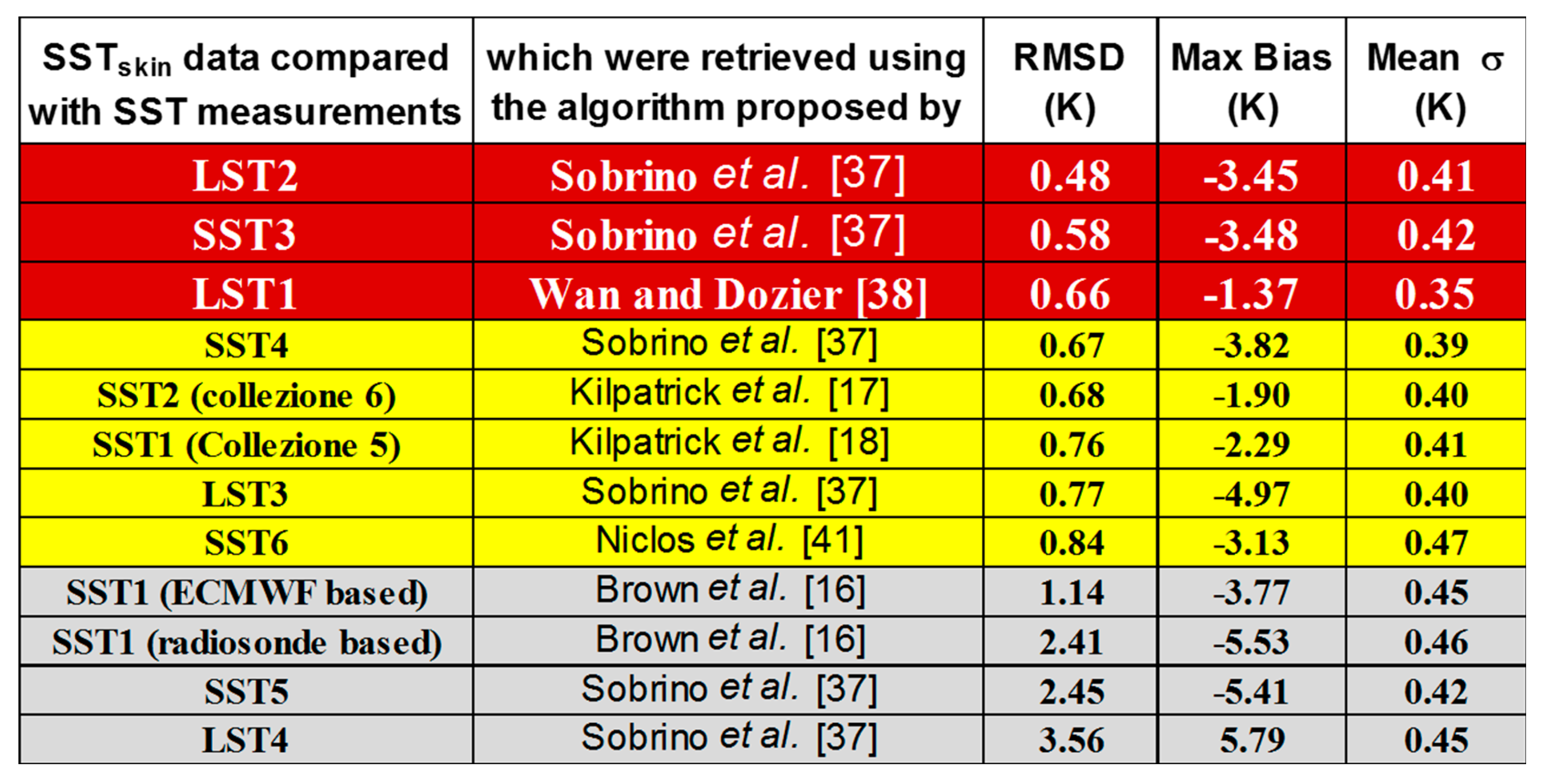
LST2 measurements, which were obtained with the algorithm for retrieving LST data from MODIS images proposed by Sobrino et al. [37], showed the smallest RMSD value, i.e., 0.48 K, and a maximum bias equal to −3.45 K and σ value equal to 0.41 K (Figure 2). LST1 measurements, which were calculated with the current operational algorithm for retrieving LST data from MODIS images [38], showed an RMSD value greater than the one from the LST2 data and was slightly smaller than the one from the SST2(collection 6) data, which were calculated with the current operational algorithm for retrieving SST data from MODIS images [17], i.e., 0.66 K (Figure 2). However, the LST1 measurements highlighted the smallest values of the maximum bias and σ, i.e., −1.37 K and 0.35 K, respectively (Figure 2). Both methods were successfully applied to retrieve the LST data and include the SSE values in their equations. The method described by Sobrino et al. [37] also included W content, whereas coefficients of the Wan and Dozier [38] algorithm were dependent on water vapor content. It is important to underline that water vapor contents exploited to identify the coefficients of the algorithm [38] were acquired with AERONET instruments, whereas the W contents included in retrieval of LST2 measurements were estimated from MODIS images. These values were validated with AERONET data (R2 is equal to 0.717 [13]).
Moreover, the SST3 measurements, which were obtained with the linear SW algorithm for retrieving SST data from MODIS images proposed by Sobrino et al. [37], showed a RMDS value greater than the one from the LST2 data and smaller than the ones from the LST1 and SST2(collection 6) data, i.e., 0.58 K (Figure 2). However, the SST3 measurements highlighted maximum bias and σ values greater than the ones from LST1 and SST2(collection 6) data, i.e., −3.48 K and 0.42 K, respectively (Figure 2). SS4 measurements obtained with the linear SW algorithm for retrieving SST data from MODIS images proposed by Sobrino et al. [37], showed an RMDS value slightly greater than the one from LST1 data, and slightly smaller than the one from SST2(collection 6) data, i.e., 0.67 K (Figure 2). However, the SST4 measurements highlighted a maximum bias greater than the one from the LST1 and SST2(collection 6) data, i.e., −3.82 K, and σ value greater than the one from the LST1 data and smaller than the ones from the LST2 and SST2(collection 6) data, i.e., 0.39 K, (Figure 2). Both methods were the linear SW algorithms successfully applied to retrieve SST data, and the SST4 measurements were evaluated including total atmospheric water vapor content.
As above-mentioned, the LST1 measurements highlighted the smallest value of σ, i.e., 0.35 K (Figure 2). The LST2, SST3, SST4, SST2(collection 6), SST2(collection 5), LST3, and SST5 data showed comparable values of σ from 0.42 K to 0.39 K (Figure 2). Therefore, the reduction of the error in the SST data of LST2, SST3, SST4, SST2(collection 6), SST2(collection 5), and LST3 measurements can be considered uniform.
The comparison of RMDS values highlighted that LST2, SST3, LST1, and SST4 data reduced the error in SST measurements in these coastal waters with respect to SST2(collection 6) data, which were calculated with the current operational algorithm for retrieving global data of SST from MODIS images [17]. Moreover, σ values of LST1 and SST4 data were smaller than the one from SST2(collection 6) measurements, i.e., 0.35 K, 0.39 K, and 0.40 K, respectively; and the maximum bias of LST1 data was smaller than the one from SST2(collection 6) measurements, i.e., −1.37 K and −1.90 K, respectively. It should be noted that the operation algorithms do not perform well in coastal situations since they were developed to produce global measurement of SST and the atmospheric correction algorithms were optimized for oceanic conditions [16,17,18,19].
It is interesting to note that the current operation algorithms for retrieving LST and SST data from MODIS bands 31 and 32 highlighted the smallest values of the maximum bias, –1.37 K and –1.90 K, respectively.
The comparisons between the SSTskin data and SST1(radiosonde based), SST1(ECMWF based), SST1(collection 5), and SST1(collection 6) measurements obtained with the operation algorithms for retrieving SST data from MODIS bands 31 and 32, highlighted that changes in coefficients and algorithms improved the accuracy of SST data in these coastal waters. The RMSD values reduced from 2.41 to 0.68 K, the maximum biases decreased from −5.53 to −1.90 K, and values of σ reduced from 0.46 to 0.40 K (Figure 2).
5. Conclusions
SSTskin measurements of coastal waters of the Manfredonia Gulf, Taranto Gulf, and the area close to Lesina Lagoon were compared with SST measurements retrieved from MODIS images. The retrieval of SST data was performed with three sets of SW algorithms: (i) not-linear SST methods (i.e., Equations (1) and (2)) developed and modified by an international team of scientists employed to produce global SST measurements from MODIS data; (ii) four well-tested algorithms for retrieving SST data from MODIS images (i.e., Equations (3)–(6)) proposed by [37,41]. Sobrino et al. [37] introduced two linear SW techniques, one of these with terms dependent on W content (Equation (4)), and a linear quadratic algorithm (Equation (5)). Niclòs et al. [41] proposed a quadratic regression that included W and SSE values (Equation (6)); and (iii) four algorithms for retrieving LST data from MODIS images (Equations (7)–(10)) where W and LSE values were taken into consideration. The international team of scientists employed to produce accurate LST measurements proposed Equation (7). Sobrino et al. [37] introduced Equations (8)–(10) to retrieve LST measurements from MODIS data.
The comparison with the SSTskin evaluated from in situ data highlighted that the algorithm for retrieving LST data from MODIS images proposed by Sobrino et al. [37] and the current operative algorithm for retrieving LST data from MODIS images proposed by Wan and Dozier [38] both minimized the error in the SST measurements of these coastal waters with respect to the current operative algorithm for retrieving global data of SST from MODIS images proposed by Kilpatrick et al. [17].
Therefore, the results demonstrate that SW algorithms for retrieving LST measurements that include W and SSE values can improve the accuracy of SST measurements in near-land coastal waters. Furthermore, the variation in W and SSE values of near-land coastal waters can be considered comparable to the variation of other land surfaces.
Future work should aim to exploit the variations in W and SSE values for further reducing the error in SST measurements in near-land coastal waters.
Acknowledgments
This research was supported by the Italian National Research Council. The author thanks the Principal Investigators and their staff for establishing and maintaining the six AERONET sites used in this investigation. The author would like to thank Sean Bailey, Otis Brown, Peter J. Minnett, and Katherine Kilpatrick for their valuable comments and suggestions and their useful corrections which improved the quality of this manuscript. The author is particularly grateful to Zhengming Wan.
Conflicts of Interest
The author declares no conflict of interest
References
- Blanchette, C.A.; Miner Melis, C.; Raimondi, P.T.; Lohse, D.; Heady, K.E.; Broitman, B.R. Biogeographical patterns of rocky intertidal communities along the Pacific coast of North America. J. Biogeogr. 2008, 35, 1593–1607. [Google Scholar] [CrossRef]
- Ahuja, S. Monitoring Water Quality: Pollution Assessment, Analysis, and Remediation; Elsevier: Waltham, MA, USA, 2013; pp. 1–379. [Google Scholar]
- Smale, D.A.; Wernberg, T. Satellite-derived SST data as a proxy for water temperature in nearshore benthic ecology. Mar. Ecol. Prog. Ser. 2009, 387, 27–37. [Google Scholar] [CrossRef]
- Valentini, E.; Filipponi, F.; Nguyen Xuan, A.; Passarelli, F.M.; Taramelli, A. Earth Observation for Maritime Spatial Planning: Measuring, Observing and Modeling Marine Environment to Assess Potential Aquaculture Sites. Sustainability 2016, 8, 519. [Google Scholar] [CrossRef]
- McCaul, M.; Barland, J.; Cleary, J.; Cahalane, C.; McCarthy, T.; Diamond, D. Combining Remote Temperature Sensing with in-Situ Sensing to Track Marine/Freshwater Mixing Dynamics. Sensors 2016, 16, 1402. [Google Scholar] [CrossRef] [PubMed]
- Narváez, D.A.; Poulin, E.; Leiva, G.; Hernández, E.; Castilla, J.C.; Navarrete, S.A. Seasonal and spatial variation of nearshore hydrographic conditions in central Chile. Cont. Shelf Res. 2004, 24, 279–292. [Google Scholar] [CrossRef]
- De Boer, G.J.; Pietrzak, J.D.; Winterwerp, J.C. SST observations of upwelling induced by tidal straining in the Rhine ROFI. Cont. Shelf Res. 2009, 29, 263–277. [Google Scholar] [CrossRef]
- Tang, D.; Kester, D.R.; Wang, Z.; Lian, J.; Kawamura, H. AVHRR satellite remote sensing and shipboard measurements of the thermal plume from the Daya Bay, nuclear power station, China. Remote Sens. Environ. 2003, 84, 506–515. [Google Scholar] [CrossRef]
- Dufois, F.; Penven, P.; Whittle, C.P.; Veitch, J. On the warm nearshore bias in Pathfinder monthly SST products over Eastern Boundary Upwelling Systems. Ocean Model. 2012, 47, 113–118. [Google Scholar] [CrossRef]
- Castillo, K.D.; Lima, F.P. Comparison of in situ and satellite-derived (MODIS-Aqua/Terra) methods for assessing temperatures on coral reefs. Limnol. Oceanogr. Methods 2010, 8, 107–117. [Google Scholar] [CrossRef]
- Leichter, J.J.; Helmuth, B.; Fischer, A.M. Variation beneath the surface: Quantifying complex thermal environments on coral reefs in the Caribbean, Bahamas and Florida. J. Mar. Res. 2006, 64, 563–588. [Google Scholar] [CrossRef]
- Thomas, A.; Byrne, D.; Weatherbee, R. Coastal sea surface temperature variability from Landsat infrared data. Remote Sens. Environ. 2002, 81, 262–272. [Google Scholar] [CrossRef]
- Cavalli, R.M. Retrieval of Sea Surface Temperature from MODIS Data in Coastal Waters. Sustainability 2017, 9, 2032. [Google Scholar] [CrossRef]
- Pearce, A.; Faskel, F.; Hyndes, G. Nearshore sea temperature variability off Rottnest Island (Western Australia) derived from satellite data. Int. J. Remote Sens. 2006, 27, 2503–2518. [Google Scholar] [CrossRef]
- Smit, A.J.; Roberts, M.; Anderson, R.J.; Dufois, F.; Dudley, S.F.; Bornman, T.G.; Bolton, J.J. A Coastal Seawater Temperature Dataset for Biogeographical Studies: Large Biases between In Situ and Remotely-Sensed Data Sets around the Coast of South Africa. PLoS ONE 2013, 8, e81944. [Google Scholar] [CrossRef] [PubMed] [Green Version]
- Brown, O.B.; Minnett, P.J.; Evans, R.; Kearns, E.; Kilpatrick, K.; Kumar, A.; Sikorski, R.; Závody, A. MODIS Infrared Sea Surface Temperature Algorithm Algorithm Theoretical Basis Document; Version 2.0; University of Miami: Miami, FL, USA, 1999; pp. 1–91. [Google Scholar]
- Kilpatrick, K.; Podesta, G.; Walsh, S.; Evans, R.; Minnett, P. Implementation of Version 6 AQUA and TERRA SST Processing; White Paper; University of Miami: Coral Gables, FL, USA, 2014. [Google Scholar]
- Kilpatrick, K.A.; Podestá, G.; Walsh, S.; Williams, E.; Halliwell, V.; Szczodrak, M.; Brown, O.B.; Minnett, P.J.; Evans, R. A decade of sea surface temperature from MODIS. Remote Sens. Environ. 2015, 165, 27–41. [Google Scholar] [CrossRef]
- Szczodrak, M.; Minnett, P.J.; Evans, R.H. The effects of anomalous atmospheres on the accuracy of infrared sea-surface temperature retrievals: Dry air layer intrusions over the tropical ocean. Remote Sens. Environ. 2014, 140, 450–465. [Google Scholar] [CrossRef]
- Fiedler, L.; Bakan, S. Interferometric measurements of sea surface temperature and emissivity. Deutsch. Hydrogr. Z. 1997, 49, 357–365. [Google Scholar] [CrossRef]
- Friedman, D. Infrared characteristics of ocean water (1.5–15 μ). Appl. Opt. 1969, 8, 2073–2078. [Google Scholar] [CrossRef] [PubMed]
- Konda, M.; Imasato, N.; Nishi, K.; Toda, T. Measurement of the sea surface emissivity. J. Oceanogr. 1994, 50, 17–30. [Google Scholar] [CrossRef]
- Masuda, K.; Takashima, T.; Takayama, Y. Emissivity of pure and sea waters for the model sea surface in the infrared window regions. Remote Sens. Environ. 1988, 24, 313–329. [Google Scholar] [CrossRef]
- Masuda, K. Influence of wind direction on the infrared sea surface emissivity model including multiple reflection effect. Meteorol. Geophys. 2012, 63, 1–13. [Google Scholar] [CrossRef]
- Newman, S.M.; Smith, J.A.; Glew, M.D.; Rogers, S.M.; Taylor, J.P. Temperature and salinity dependence of sea surface emissivity in the thermal infrared. Q. J. R. Meteorol. Soc. 2005, 131, 2539–2557. [Google Scholar] [CrossRef]
- Niclòs, R.; Caselles, V. Angular variation of the sea surface emissivity. In Recent Research Development in Thermal Remote Sensing; Research Signpost: Thiruvananthapuram, Indian, 2005; pp. 37–65. [Google Scholar]
- Niclòs, R.; Caselles, V.; Coll, C.; Valor, E.; Rubto, E. Autonomous Measurements of Sea Surface Temperature Using In Situ Thermal Infrared Data. J. Atmos. Ocean. Technol. 2004, 21, 683–692. [Google Scholar] [CrossRef]
- Niclòs, R.; Valor, E.; Caselles, V.; Coll, C.; Sánchez, J.M. In situ angular measurements of thermal infrared sea surface emissivity—Validation of models. Remote Sens. Environ. 2005, 94, 83–93. [Google Scholar] [CrossRef]
- Salisbury, J.W. Emissivity of terrestrial materials in the 8–14 μm atmospheric window. Remote Sens. Environ. 1992, 42, 83–106. [Google Scholar] [CrossRef]
- Watts, P.D.; Allen, M.R.; Nightingale, T.J. Wind speed effects on sea surface emission and reflection for the along track scanning radiometer. J. Atmos. Ocean. Technol. 1996, 13, 126–141. [Google Scholar] [CrossRef]
- Wen-Yao, L.; Field, R.T.; Gantt, R.G.; Klemas, V. Measurement of the surface emissivity of turbid waters. Remote Sens. Environ. 1987, 21, 97–109. [Google Scholar] [CrossRef]
- Wei, J.A.; Wang, D.; Gong, F.; He, X.; Bai, Y. The Influence of Increasing Water Turbidity on Sea Surface Emissivity. IEEE Trans. Geosci. Remote Sens. 2017, 55, 3501–3515. [Google Scholar] [CrossRef]
- Wu, X.; Smith, W.L. Emissivity of rough sea surface for 8–13 μm: Modeling and verification. Appl. Opt. 1997, 36, 2609–2619. [Google Scholar] [CrossRef] [PubMed]
- Mueller, J.L.; Austin, R.W.; Morel, A.; Fargion, G.S.; McClain, C.R. Ocean Optics Protocols for Satellite Ocean Color Sensor Validation, Revision 4, Volume I: Introduction, Background and Conventions; NASA Technical Memorandum 2003-21621; NASA Goddard Space Flight Center: Greenbelt, MD, USA, 2003; pp. 1–56.
- Wolfe, R.E.; Roy, D.P.; Vermote, E. MODIS land data storage, gridding, and compositing methodology: Level 2 grid. IEEE Trans. Geosci. Remote Sens. 1998, 36, 1324–1338. [Google Scholar] [CrossRef]
- Becker, F.; Li, Z.L. Towards a local split window method over land surfaces. Remote Sens. 1990, 11, 369–393. [Google Scholar] [CrossRef]
- Sobrino, J.A.; El Kharraz, J.; Li, Z.L. Surface temperature and water vapour retrieval from MODIS data. Int. J. Remote Sens. 2003, 24, 5161–5182. [Google Scholar] [CrossRef]
- Wan, Z.M.; Dozier, J. A generalized split-window algorithm for retrieving land surface temperature from space. IEEE Trans. Geosci. Remote Sens. 1996, 34, 892–905. [Google Scholar]
- Wan, Z. MODIS Land-Surface Temperature Algorithm Theoretical Basis Document (LST ATBD); Version 3.3; University of California: Santa Barbara, CA, USA, 1999. [Google Scholar]
- Emery, W.J.; Yu, Y.; Wick, G.A.; Schluessel, P.; Reynolds, R.W. Correcting infrared satellite estimates of sea surface temperature for atmospheric water vapor attenuation. J. Geophys. Res. Oceans 1994, 99, 5219–5236. [Google Scholar] [CrossRef]
- Niclòs, R.; Caselles, V.; Coll, C.; Valor, E. Determination of sea surface temperature at large observation angles using an angular and emissivity-dependent split-window equation. Remote Sens. Environ. 2007, 111, 107–121. [Google Scholar] [CrossRef]
- Cavalli, R.M.; Betti, M.; Campanelli, A.; Di Cicco, A.; Guglietta, D.; Penna, P.; Piermattei, V. A methodology to assess the accuracy with which remote data characterize a specific surface, as a Function of Full Width at Half Maximum (FWHM): Application to three Italian coastal waters. Sensors 2014, 14, 1155–1183. [Google Scholar] [CrossRef] [PubMed]
- Cattaneo, A.; Correggiari, A.; Langone, L.; Trincardi, F. The late-Holocene Gargano subaqueous delta. Adriatic shelf: Sediment pathways and supply fluctuations. Mar. Geol. 2003, 193, 61–91. [Google Scholar] [CrossRef]
- Monticelli, L.S.; Caruso, G.; Decembrini, F.; Caroppo, C.; Fiesoletti, F. Role of prokaryotic biomasses and activities in carbon and phosphorus cycles at a coastal. thermohaline front and in offshore waters (Gulf of Manfredonia. Southern Adriatic Sea). Microb. Ecol. 2014, 67, 501–519. [Google Scholar] [CrossRef] [PubMed]
- Spagnoli, F.; Dell’Anno, A.; De Marco, A.; Dinelli, E.; Fabiano, M.; Gadaleta, M.V.; Iannig, C.; Loiaconoc, F.; Maninia, M.; Mongelli, G.; et al. Biogeochemistry, grain size and mineralogy of the central and southern Adriatic Sea sediments: A review. Chem. Ecol. 2010, 26 (Suppl. 1), 19–44. [Google Scholar] [CrossRef] [Green Version]
- Rebesco, M.; Neagu, R.C.; Cuppari, A.; Muto, F.; Accettella, D.; Dominici, R.; Caburlotto, A. Morphobathymetric analysis and evidence of submarine mass movements in the western Gulf of Taranto (Calabria margin. Ionian Sea). Int. J. Earth Sci. 2009, 98, 791–805. [Google Scholar] [CrossRef]
- Buccolieri, A.; Buccolieri, G.; Cardellicchio, N.; Dell’Atti, A.; Di Leo, A.; Maci, A. Heavy metals in marine sediments of Taranto Gulf (Ionian Sea. southern Italy). Mar. Chem. 2006, 99, 227–235. [Google Scholar] [CrossRef]
- Cardellicchio, N.; Buccolieri, A.; Di Leo, A.; Giandomenico, S.; Spada, L. Levels of metals in reared mussels from Taranto Gulf (Ionian Sea. Southern Italy). Food Chem. 2008, 107, 890–896. [Google Scholar] [CrossRef]
- Cattaneo, A.; Trincardi, F.; Asioli, A.; Correggiari, A. The Western Adriatic shelf clinoform: Energy-limited bottomset. Cont. Shelf Res. 2007, 27, 506–525. [Google Scholar] [CrossRef]
- Roselli, L.; Fabbrocini, A.; Manzo, C.; D’Adamo, R. Hydrological heterogeneity, nutrient dynamics and water quality of a non-tidal lentic eco system (Lesina Lagoon, Italy). Estuar. Coast. Shelf Sci. 2009, 84, 539–552. [Google Scholar] [CrossRef]
- Crease, J.; Dauphinee, T.; Grose, P.L.; Lewis, E.L.; Fofonoff, N.P.; Plakhin, E.A.; Striggow, K.; Zenk, W. The Acquisition, Calibration and Analysis of CTD Data; UNESCO Technical Papers in Marine Sciences: Paris, France, 1988; Volume 54, pp. 1–105. [Google Scholar]
- Webster, P.J.; Clayson, C.A.; Curry, J.A. Clouds, radiation, and the diurnal cycle of sea surface temperature in the tropical western Pacific. J. Clim. 1996, 9, 1712–1730. [Google Scholar] [CrossRef]
- Fairall, C.W.; Bradley, E.F.; Hare, J.E.; Grachev, A.A.; Edson, J.B. Bulk parameterization of air–sea fluxes: Updates and verification for the COARE algorithm. J. Clim. 2003, 16, 571–591. [Google Scholar] [CrossRef]
- Donlon, C.J.; Keogh, S.J.; Baldwin, D.J.; Robinson, I.S.; Ridley, I.; Sheasby, T.; Barton, I.J.; Bradley, E.F.; Nightingale, T.J.; Emery, W. Solid-State Radiometer Measurements of Sea Surface Skin Temperature. J. Atmos. Ocean. Technol. 1998, 15, 775–787. [Google Scholar] [CrossRef]
- Fairall, C.W.; Bradley, E.F.; Godfrey, J.S.; Wick, G.A.; Edson, J.B.; Young, G.S. Cool-skin and warm-layer effects on sea surface temperature. J. Geophys. Res. Oceans 1996, 101, 1295–1308. [Google Scholar] [CrossRef]
- Kawai, Y.; Wada, A. Diurnal sea surface temperature variation and its impact on the atmosphere and ocean: A review. J. Oceanogr. 2007, 63, 721–744. [Google Scholar] [CrossRef]
- Gentemann, C.L.; Minnett, P.J.; Ward, B. Profiles of ocean surface heating (POSH): A new model of upper ocean diurnal warming. J. Geophys. Res. Oceans 2009, 114, C07017. [Google Scholar] [CrossRef]
- Mueller, J.L.; McClain, G.; Bidigare, R.; Trees, C.; Balch, W.; Dore, J.; Drapeau, D.; Karl, D.; Van, L. Ocean Optics Protocols for Satellite Ocean Color Sensor Validation, Revision 5, Volume V: Biogeochemical and Bio-Optical Measurements and Data Analysis Protocols; NASA Technical Memorandum 2003-21621; NASA Goddard Space Flight Center: Greenbelt, MD, USA, 2003; pp. 1–36.
- Pegau, S.; Zaneveld, J.R.V.; Mitchell, B.G.; Mueller, J.L.; Kahru, M.; Wieland, J.; Stramska, M. Ocean Optics Protocols For Satellite Ocean Color Sensor Validation, Revision 4, Volume IV: Inherent Optical Properties: Instruments, Characterizations, Field Measurements and Data Analysis Protocols; NASA Technical Memorandum 2003-211621; NASA Goddard Space Flight Center: Greenbelt, MD, USA, 2003; pp. 1–76.
- Walton, C.C. A review of differential absorption algorithms utilized at NOAA for measuring sea surface temperature with satellite radiometers. Remote Sens. Environ. 2016, 187, 434–446. [Google Scholar] [CrossRef]
- François, C.; Brisson, A.; Le Borgne, P.; Marsouin, A. Definition of a radiosounding database for sea surface brightness temperature simulations: Application to sea surface temperature retrieval algorithm determination. Remote Sens. Environ. 2002, 81, 309–326. [Google Scholar] [CrossRef]
Figure 1.
Study area: (a) study area locations (the red, green, and cyan shapes delimit coastal waters of the Manfredonia Gulf, Taranto Gulf, and the area close to Lesina Lagoon, respectively); (b) the measurement locations of coastal waters of the Manfredonia Gulf; (c) seafloor morphology of the Manfredonia Gulf; (d) measurement locations of coastal waters of the Taranto Gulf; (e) seafloor morphology of the Taranto Gulf; (f) measurement locations of coastal waters close to Lesina Lagoon; and (g) seafloor morphology of coastal waters close to Lesina Lagoon.
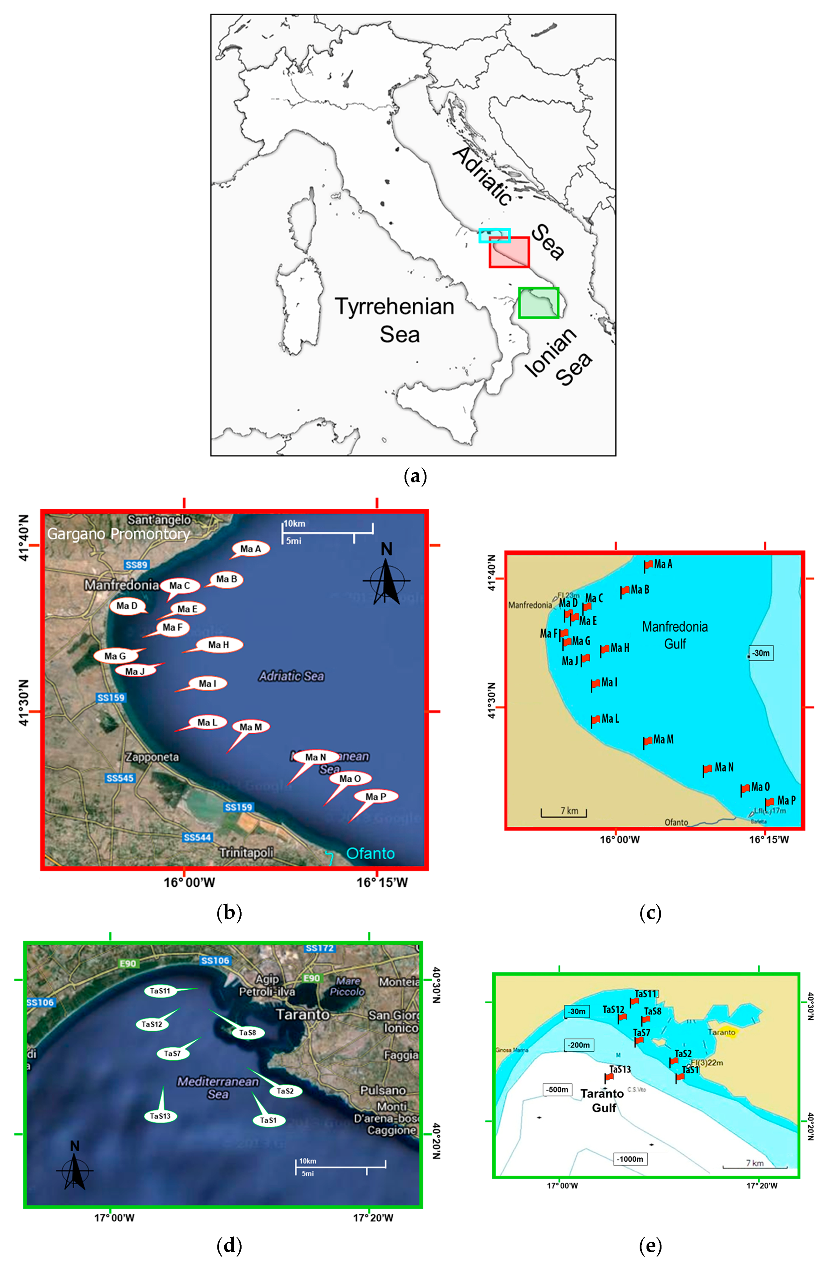
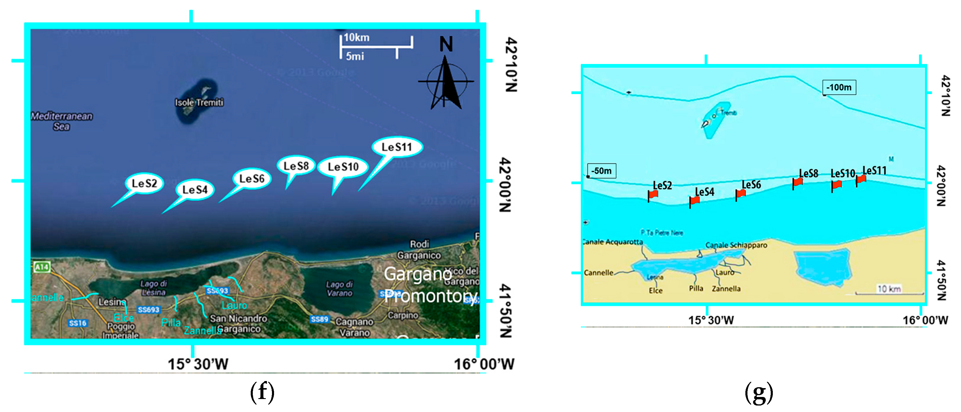
Figure 2.
The ranking of split window (SW) techniques for retrieving land surface temperature (LST) and sea surface temperature (SST) measurements from MODIS images based on root-mean-square deviation (RMDS) values between SSTskin data and SST1(radiosonde based), SST1(ECMWF based), SST1(collection 5), SST2(collection 6), SST3, SST4, SST5, SST6, LST1, LST2, LST3, and LST4 measurements.


Table 1.
Date and start time of the moderate resolution imaging spectroradiometer (MODIS) overpasses, number of observations monitored within ±2 h with respect to MODIS overpasses, means, and standard deviations (σ) of SPM and salinity concentrations, and SSTskin measurements.
Table 1.
Date and start time of the moderate resolution imaging spectroradiometer (MODIS) overpasses, number of observations monitored within ±2 h with respect to MODIS overpasses, means, and standard deviations (σ) of SPM and salinity concentrations, and SSTskin measurements.
| Coastal Waters of the Manfredonia Gulf | ||||||
| Date | Start Time (UTC) | Number of Locations | SPM (mg/L) | Salinity (g/L) | SSTskin (K) | |
| 08/08/2011 | 11:45 | 5 | Mean | 3.01 | 38.22 | 301.10 |
| σ | 1.82 | 0.06 | 0.69 | |||
| 09/08/2011 | 12:25 | 7 | Mean | 3.16 | 38.17 | 301.22 |
| σ | 0.75 | 0.04 | 0.55 | |||
| 12/08/2011 | 11:20 | 8 | Mean | 5.42 | 38.33 | 299.79 |
| σ | 2.24 | 0.07 | 0.38 | |||
| 24/08/2011 | 11:40 | 11 | Mean | 7.44 | 38.41 | 301.86 |
| σ | 0.86 | 0.04 | 0.51 | |||
| Coastal Waters of the Taranto Gulf | ||||||
| Date | Start Time (UTC) | Number of Locations | SPM (mg/L) | Salinity (g/L) | SSTskin (K) | |
| 13/08/2011 | 12:00 | 5 | Mean | 2.36 | 38.31 | 299.47 |
| σ | 0.58 | 0.01 | 0.34 | |||
| 14/08/2011 | 12:45 | 6 | Mean | 1.93 | 38.29 | 300.25 |
| σ | 0.63 | 0.04 | 0.42 | |||
| 15/08/2011 | 11:50 | 6 | Mean | 2.37 | 38.30 | 299.81 |
| σ | 0.56 | 0.06 | 0.42 | |||
| 16/08/2011 | 12:30 | 2 | Mean | 1.69 | 38.23 | 299.99 |
| σ | 0.11 | 0.01 | 0.26 | |||
| Coastal Waters of the Area Close to Lesina Lagoon | ||||||
| Date | Start Time (UTC) | Number of Locations | SPM (mg/L) | Salinity (g/L) | SSTskin (K) | |
| 07/08/2011 | 12:40 | 6 | Mean | 1.50 | 37.86 | 300.12 |
| σ | 0.41 | 0.08 | 0.21 | |||
Table 2.
Values of root-mean-square deviation (RMSD), bias, and σ between SSTskin data and SST1(radiosonde based), SST1(ECMWF based), and SST1(collection 5) measurements.
Table 2.
Values of root-mean-square deviation (RMSD), bias, and σ between SSTskin data and SST1(radiosonde based), SST1(ECMWF based), and SST1(collection 5) measurements.
| Date Start Time | SST1(radiosonde based) (K) | SST1(ECMWF based) (K) | SST1(collection 5) (K) | SST2(collection 6) (K) | |
|---|---|---|---|---|---|
| Coastal Waters of the Manfredonia Gulf | |||||
| 08/08/2011 11:45 UTC | Bias | −2.19 ** | −0.78 ** | −0.28 # | 0.25 # |
| σ | 0.33 | 0.35 | 0.67 | 0.65 | |
| RMSD | 2.21 | 0.84 | 0.67 | 0.65 | |
| 09/08/2011 12:25 UTC | Bias | −2.57 ** | −0.93 ** | −0.19 # | 0.27 # |
| σ | 0.94 | 0.97 | 0.91 | 0.95 | |
| RMSD | 2.71 | 1.30 | 0.88 | 0.93 | |
| 12/08/2011 11:20 UTC | Bias | −4.19 ** | −1.16 ** | 0.64 * | 1.02 * |
| σ | 0.30 | 0.27 | 0.30 | 0.31 | |
| RMSD | 4.20 | 1.18 | 0.70 | 1.06 | |
| 24/08/2011 11:40 UTC | Bias | −1.26 ** | −0.76 ** | 0.66 * | 0.30 * |
| σ | 0.30 | 0.31 | 0.34 | 0.32 | |
| RMSD | 1.30 | 0.82 | 0.74 | 0.43 | |
| Coastal Waters of the Taranto Gulf | |||||
| 13/08/2011 12:00 UTC | Bias | −2.46 ** | −1.42 ** | −0.84 ** | −0.59 ** |
| σ | 0.15 | 0.13 | 0.12 | 0.12 | |
| RMSD | 2.47 | 1.42 | 0.85 | 0.60 | |
| 14/08/2011 12:45 UTC | Bias | −3.12 ** | −1.37 ** | 0.83 * | 0.61 * |
| σ | 1.16 | 1.10 | 0.23 | 0.22 | |
| RMSD | 3.30 | 1.70 | 0.85 | 0.65 | |
| 15/08/2011 11:50 UTC | Bias | −2.12 ** | −1.02 ** | −0.74 ** | −0.48 ** |
| σ | 0.37 | 0.35 | 0.32 | 0.31 | |
| RMSD | 2.15 | 1.07 | 0.80 | 0.56 | |
| 16/08/2011 12:30 UTC | Bias | −1.59 ** | −0.82 ** | 0.46 * | 0.41 * |
| σ | 0.03 | 0.06 | 0.11 | 0.11 | |
| RMSD | 1.59 | 0.82 | 0.47 | 0.42 | |
| Coastal Waters of the Area Close to Lesina Lagoon | |||||
| 07/08/2011 12:40 UTC | Bias | −1.46 ** | −1.11 ** | 0.57 # | 0.52 # |
| σ | 0.27 | 0.28 | 0.47 | 0.44 | |
| RMSD | 1.48 | 1.14 | 0.71 | 0.66 | |
* all values of bias are warm, i.e., SST data retrieved from satellite images are greater than ones measured in situ; ** all values of bias are cold; # bias values are both warm and cold.
Table 3.
Values of RMSD, bias, and σ between SSTskin data and SST3, SST4, SST5, and SST6 measurements.
Table 3.
Values of RMSD, bias, and σ between SSTskin data and SST3, SST4, SST5, and SST6 measurements.
| Date Start Time | SST3 (K) | SST4 (K) | SST5 (K) | SST6 (K) | |
|---|---|---|---|---|---|
| Coastal Waters of the Manfredonia Gulf | |||||
| 08/08/2011 11:45 UTC | Bias | −0.36 # | 0.48 # | 0.63 * | −0.72 # |
| σ | 0.39 | 0.41 | 0.47 | 0.43 | |
| RMSD | 0.51 | 0.61 | 0.76 | 0.82 | |
| 09/08/2011 12:25 UTC | Bias | −0.49 # | 0.43 # | 4.21 * | −0.72 # |
| σ | 0.99 | 1.01 | 1.09 | 1.09 | |
| RMSD | 1.05 | 1.04 | 9.67 | 1.26 | |
| 12/08/2011 11:20 UTC | Bias | −0.35 # | −0.50 # | −1.91 ** | −0.79 # |
| σ | 0.29 | 0.30 | 0.27 | 0.52 | |
| RMSD | 0.45 | 0.58 | 1.92 | 0.93 | |
| 24/08/2011 11:40 UTC | Bias | −0.34 # | −0.55 # | −0.73 ** | −0.69 ** |
| σ | 0.32 | 0.31 | 0.31 | 0.31 | |
| RMSD | 0.46 | 0.63 | 0.79 | 0.75 | |
| Coastal Waters of the Taranto Gulf | |||||
| 13/08/2011 12:00 UTC | Bias | −0.27 ** | −0.43 ** | −1.45 ** | −1.03 ** |
| σ | 0.12 | 0.13 | 0.13 | 0.12 | |
| RMSD | 0.29 | 0.44 | 1.45 | 1.03 | |
| 14/08/2011 12:45 UTC | Bias | −1.06 ** | −0.99 ** | −2.60 ** | −0.54 ** |
| σ | 0.25 | 0.25 | 0.41 | 0.25 | |
| RMSD | 1.09 | 1.01 | 2.63 | 0.59 | |
| 15/08/2011 11:50 UTC | Bias | −0.14 # | −0.31 # | −0.94 ** | −0.72 ** |
| σ | 0.31 | 0.30 | 0.33 | 0.32 | |
| RMSD | 0.32 | 0.42 | 0.99 | 0.78 | |
| 16/08/2011 12:30 UTC | Bias | −0.60 ** | −0.59 ** | −1.55 ** | −0.51 ** |
| σ | 0.16 | 0.12 | 0.05 | 0.07 | |
| RMSD | 0.61 | 0.60 | 1.55 | 0.52 | |
| Coastal Waters of the Area Close to Lesina Lagoon | |||||
| 07/08/2011 12:40 UTC | Bias | −0.27 # | 0.40 # | −1.56 ** | −0.49 # |
| σ | 0.41 | 0.45 | 0.48 | 0.48 | |
| RMSD | 0.46 | 0.57 | 1.62 | 0.66 | |
* all values of bias are warm; ** all values of bias are cold; # bias values are both warm and cold.
Table 4.
Values of RMSD, bias, and σ between SSTskin data and LST1, LST2, LST3, and LST4 measurements.
Table 4.
Values of RMSD, bias, and σ between SSTskin data and LST1, LST2, LST3, and LST4 measurements.
| Date Start Time | LST1 (K) | LST2 (K) | LST3 (K) | LST4 (K) | |
|---|---|---|---|---|---|
| Coastal Waters of the Manfredonia Gulf | |||||
| 08/08/2011 11:45 UTC | Bias | −0.70 ** | −0.36 # | −0.89 # | 5.25 * |
| σ | 0.29 | 0.44 | 0.35 | 0.37 | |
| RMSD | 0.75 | 0.54 | 0.94 | 5.26 | |
| 09/08/2011 12:25 UTC | Bias | −0.11 # | −0.29 # | −2.43 ** | 4.76 * |
| σ | 0.76 | 0.99 | 1.14 | 0.46 | |
| RMSD | 0.75 | 0.93 | 2.95 | 9.36 | |
| 12/08/2011 11:20 UTC | Bias | −0.91 ** | −0.04 # | −0.06 # | 1.12 # |
| σ | 0.27 | 0.40 | 0.30 | 1.02 | |
| RMSD | 0.94 | 0.38 | 0.30 | 1.48 | |
| 24/08/2011 11:40 UTC | Bias | −0.65 ** | −0.30 # | 0.00 # | 2.89 * |
| σ | 0.31 | 0.31 | 0.31 | 0.32 | |
| RMSD | 0.72 | 0.42 | 0.30 | 2.90 | |
| Coastal Waters of the Taranto Gulf | |||||
| 13/08/2011 12:00 UTC | Bias | −0.69 ** | −0.16 ** | −0.12 ** | 2.29 * |
| σ | 0.12 | 0.13 | 0.12 | 0.13 | |
| RMSD | 0.64 | 0.20 | 0.16 | 2.29 | |
| 14/08/2011 12:45 UTC | Bias | −0.34 # | −0.60 ** | −1.20 ** | 1.97 # |
| σ | 0.36 | 0.31 | 0.33 | 0.24 | |
| RMSD | 0.47 | 0.66 | 1.24 | 1.98 | |
| 15/08/2011 11:50 UTC | Bias | −0.55 # | −0.04 # | −0.04 # | 3.10 * |
| σ | 0.33 | 0.30 | 0.32 | 0.30 | |
| RMSD | 0.63 | 0.28 | 0.30 | 3.12 | |
| 16/08/2011 12:30 UTC | Bias | −0.47 # | −0.33 ** | −0.13 | 2.17 * |
| σ | 0.21 | 0.13 | 0.08 | 0.05 | |
| RMSD | 0.49 | 0.34 | 0.15 | 2.17 | |
| Coastal Waters of the Area Close to Lesina Lagoon | |||||
| 07/08/2011 12:40 UTC | Bias | −0.19 # | −0.05 # | −0.13 # | 2.06* |
| σ | 0.39 | 0.44 | 0.32 | 0.73 | |
| RMSD | 0.40 | 0.41 | 0.32 | 2.17 | |
* all values of bias are warm; ** all values of bias are cold; # bias values are both warm and cold.
© 2018 by the author. Licensee MDPI, Basel, Switzerland. This article is an open access article distributed under the terms and conditions of the Creative Commons Attribution (CC BY) license (http://creativecommons.org/licenses/by/4.0/).
Share and Cite
MDPI and ACS Style
Cavalli, R.M. Comparison of Split Window Algorithms for Retrieving Measurements of Sea Surface Temperature from MODIS Data in Near-Land Coastal Waters. ISPRS Int. J. Geo-Inf. 2018, 7, 30. https://doi.org/10.3390/ijgi7010030
AMA Style
Cavalli RM. Comparison of Split Window Algorithms for Retrieving Measurements of Sea Surface Temperature from MODIS Data in Near-Land Coastal Waters. ISPRS International Journal of Geo-Information. 2018; 7(1):30. https://doi.org/10.3390/ijgi7010030
Chicago/Turabian StyleCavalli, Rosa Maria. 2018. "Comparison of Split Window Algorithms for Retrieving Measurements of Sea Surface Temperature from MODIS Data in Near-Land Coastal Waters" ISPRS International Journal of Geo-Information 7, no. 1: 30. https://doi.org/10.3390/ijgi7010030
Note that from the first issue of 2016, this journal uses article numbers instead of page numbers. See further details here.