Identifying and Analyzing the Prevalent Regions of a Co-Location Pattern Using Polygons Clustering Approach

Abstract

Given a co-location pattern consisting of spatial features, the prevalent region mining process identifies local areas in which these features are co-located with a high probability. Many approaches have been proposed for co-location mining due to its key role in public safety, social-economic development and environmental management. However, traditionally, most of the solutions focus on itemsets mining and results outputting in a textual format, which fail to adequately treat all the spatial nature of the underlying entities and processes. In this paper, we propose a new co-location analysis approach to find the prevalent regions of a pattern. The approach combines kernel density estimation and polygons clustering techniques to specifically consider the correlation, heterogeneity and contextual information existing within complex spatial interactions. A kernel density estimation surface is created for each feature and subsequently the generated multiple surfaces are combined into a final surface with cell attribute representing the pattern prevalence measure value. Polygons consisting of cells are then extracted according to the predefined threshold. Through adding appended environmental data to the polygons, an outcome of similar groups is achieved using polygons clustering approach. The effectiveness of our approach is evaluated using Points-of-Interest datasets in Shenzhen, China.

1. Introduction

Spatial co-location pattern mining has two main purposes: (1) extracting subsets of spatial features often located together in geographic proximity [1,2,3,4,5,6]; and (2) identifying the prevalent regions of a pattern in which the features are co-located with a high probability [7,8]. This paper focuses on the second issue. It is essential to have a comprehensive and easy understanding of geographical relations, particularly under the context of the explosion of spatial data collected by sensors, location based services and scientific simulation [9,10]. Application domains of co-location patterns include environmental management, transportation, public safety, business and urban studies [6,11,12,13]. For example, the correlation between epidemic disease and stagnant water sources can be revealed by co-location mining. The connectivity relationship between terrestrial and coastal ecosystems is also interesting in terms of their co-location patterns.

Essentially, spatial co-location mining belongs to the domain of association rule mining [14,15]. It improves the transaction based approaches by incorporating the concept of spatial proximity. In the past decades, although many techniques have been proposed to extract frequent co-location patterns, most of them fail to adequately treat all the spatial nature of the underlying entities. The evaluation of spatial patterns is a difficult data analysis problem that exhibits properties of location, heterogeneity and contextual dependency. For example, rather than explicit relations stored in transaction database, spatial interactions are usually implicit in spatial database and their strength degrades in reverse proportion to distance, as stated by the Tobler’s first law of geography [16]. In addition, much useful information is hidden at the global scale, showing spatial heterogeneity across the study region [7,8,17,18]. The emphases of existing co-location mining approaches however are to materializing transactions for extracting frequent itemsets and outputting results in a textual format [4,19]. In this respect, although global relations among spatial features can be identified with traditional approaches, they may miss some valuable information at a local scale. It is necessary to identify the prevalent regions of the pattern of interest. Furthermore, classifications of prevalent regions of a pattern are generally based on the available data related to the co-location pattern itself (i.e., spatial interactions). This could limit the scope of understanding of the causes of a pattern because its prevalent regions often depend on the environmental or contextual factors (see Section 2.4).

In many cases, it is important to delimitate the prevalent regions of a co-location pattern and classify these regions by considering both factors of the location and environment. For example, chemistry contaminated water often causes human disease (e.g., breast cancer) in their nearby regions with high probability. However, due to numerous locations with human disease in the whole study region, e.g., a state, we cannot identify that human disease is strongly co-located with chemistry contaminated water using the standard global measures. For example, the global participation index PI(P) is defined as [4]:

$$\mathrm{PI}\left(P\right)={\min }_{f_i\in P}\left\{\frac{\left|\mathrm{I}\left(P,fi\right)\right|}{\left|\mathrm{I}\left(fi\right)\right|}\right\}$$

(1)

where P is the co-location pattern of interest containing feature types {f₁, f₂, …, f_k}, |I(P, f_i)| denotes the number of distinct objects of f_i in co-location instances of pattern P, and |I(f_i)| denotes the total number of objects of f_i. Pattern {chemistry contaminated water, human disease}, which could be prevalent and valuable in some local areas, tends to be diluted due to its insufficient global measure value. In spatial statistics, many useful indicators are adopted to measure pairwise co-location patterns [20,21,22]. However, it is not easy to extend these methods to handle a case with more than two variables.

As another example, different types of urban services are usually co-located in specific urban districts. Their agglomeration mechanism in local areas may be caused by their own dependency relationship or by the environmental factors such as governmental inference and local accessibility advantage. No research in the literature identifies prevalent regions for a pattern and goes on to cluster the regions based on location-based and contextual variables. Therefore, it is necessary to explore new approaches to analyze the prevalent regions of a co-location pattern with contextual information. The clustering of spatial polygons can be a key role in this issue. Expressing prevalent regions as polygons and analyzing the similarity between different polygons make the information easily understood and directly usable by domain experts, especially for the issues evolving spatial heterogeneity [23].

In general, the challenges of identifying and analyzing the prevalent regions of a co-location pattern lay in two aspects.

• Spatial heterogeneous characteristics of a co-location pattern are often neglected in previous methods [3,4,24]. They extracted co-location itemsets by measuring the prevalence of co-occurrence of spatial features in the whole study region. It is believed that many geographic processes and relations have spatial extent and should be represented by polygons in spatial database (e.g., pollution hotspots and mixed urban functional areas) [25,26]. In this paper, we propose to use kernel density estimation (KDE) to find the prevalent regions (or polygons) of a co-location pattern. Instead of using KDE for extracting frequent itemsets [27], we show that delimitating the prevalent regions of a co-location pattern can also be achieved using KDE. KDE is useful in our context as it can facilitate the representation of a co-location pattern by tessellating the study region into continuous basic units with prevalence attribute.
• In the real world, a subset of spatial features may be only prevalent in some local areas. These regions and the associated patterns are often influenced by different factors, e.g., spatial interactions and environmental variables. Existing approaches focus on the co-location scoping or the prevalent regions identifying [7,8], lacking of further support of classifying these regions to find the shared common cause(s) between them. In this paper, we investigate the contextual variables in order to develop a comprehensive understanding of the pattern at work. We propose a polygon-based clustering approach. The approach is an extension of the point-based clustering solution. It first generates polygons from multiple point datasets using KDE techniques. Then, it employs a density-based clustering algorithm with polygonal dissimilarity function to cluster the polygons which correspond to the prevalent regions of the pattern of interest. Although Flouvat et al. [2] also introduced a point-based clustering approach to summarize co-locations, their approach is based only on the location-based variable. The polygonal dissimilarity function used in our approach incorporates both location-based and contextual variables to measure the distance between prevalent regions.

The rest of this paper is organized as follows. Section 2 introduces our framework, including the techniques of KDE and polygons clustering for scoping a co-location pattern. Section 3 evaluates our approach with case studies on the dependency of urban services in Shenzhen city, China. Section 4 concludes our work and suggests future directions.

2. Polygons Clustering and Analysis for Mining Co-Location Patterns

This section firstly introduces our framework in Section 2.1. Section 2.2 and Section 2.3 then explain in detail the major procedures of the framework.

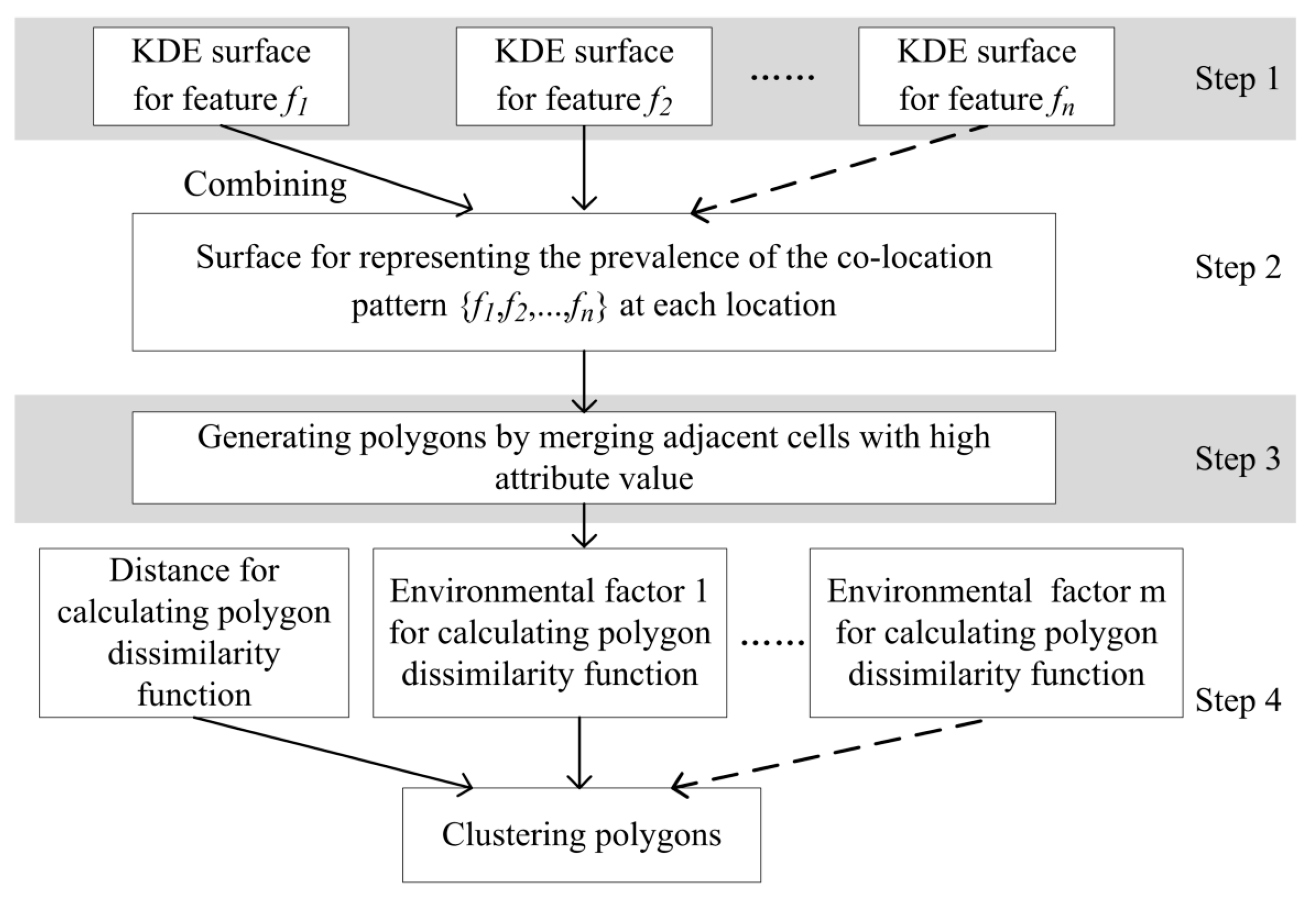
2.1. Framework

The proposed framework consists of four steps (Figure 1). It employs KDE and polygons clustering techniques to identify and analyze prevalent regions of a co-location pattern from multiple point datasets:

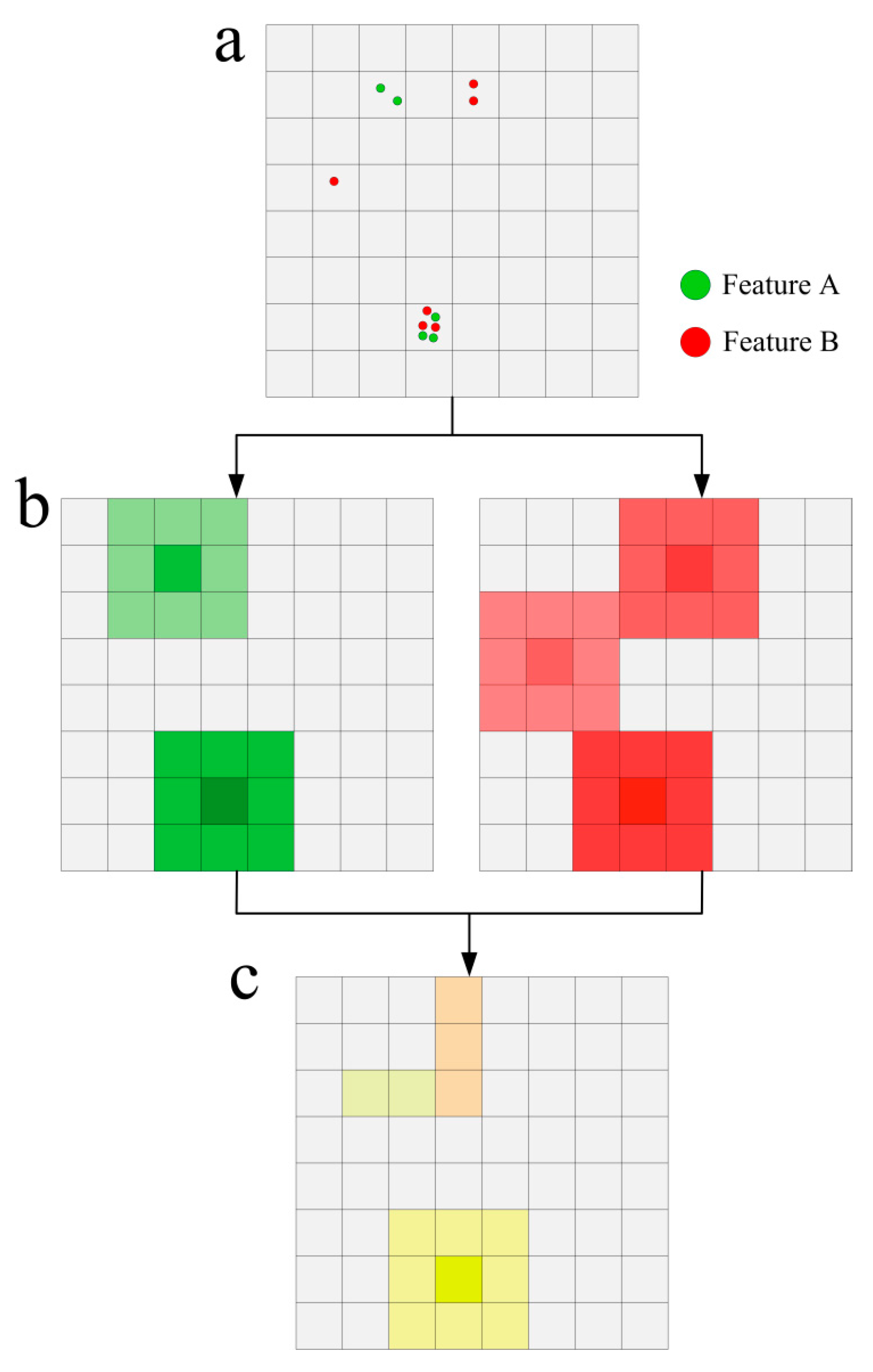
Step 1.

Generate a KDE surface for each feature evolving in the given pattern {f₁, f₂, …, f_k} (Section 2.2). After this step, multiple grids with density attribute are achieved for representing the intensity distribution of events.

Step 2.

Combine multiple KDE surfaces into a final surface with prevalence attribute, which represents the prevalence or strength of the pattern at different locations (Section 2.3). In this step, the local prevalence measure is implemented.

Step 3.

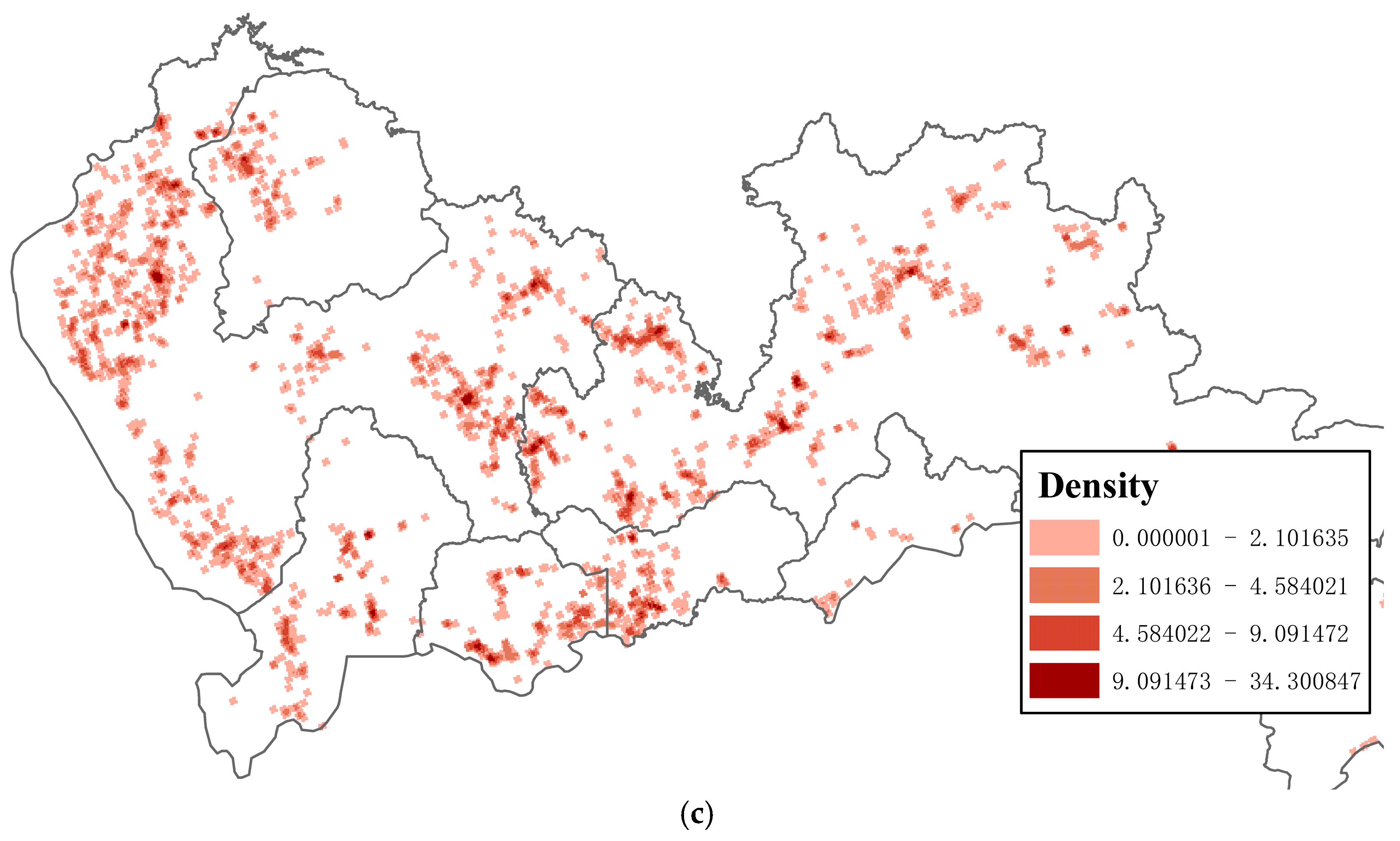
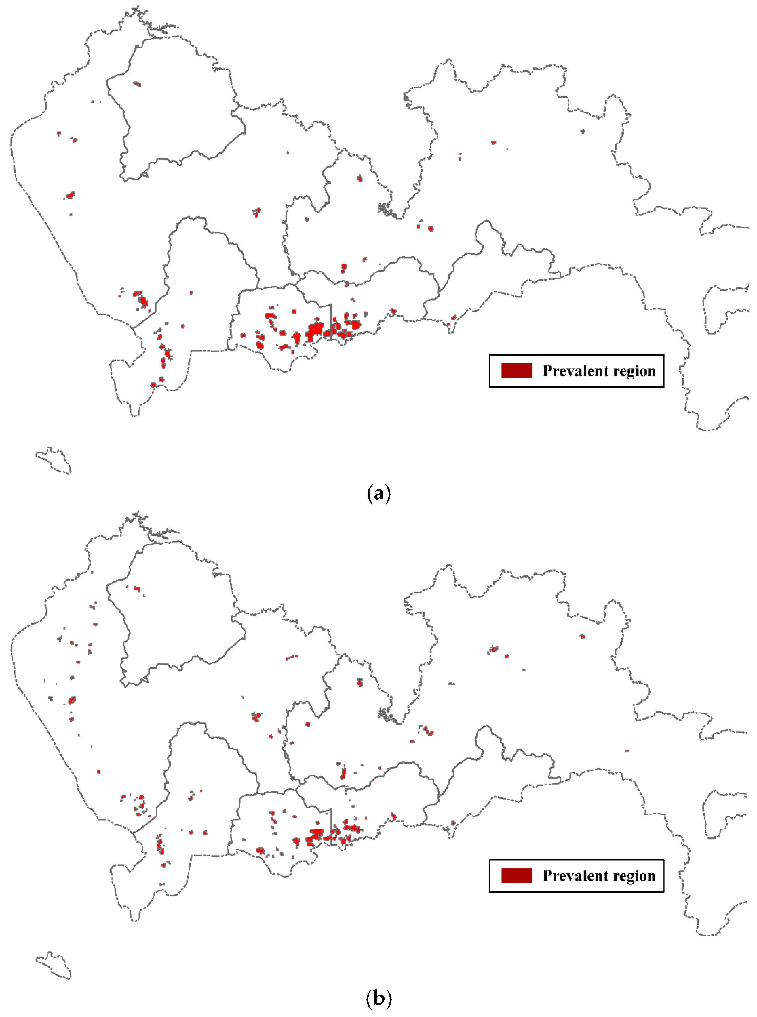
Generate polygons from the prevalence surface by merging adjacent cells with attribute value equal to or larger than the predefined threshold (Section 2.3).

Step 4.

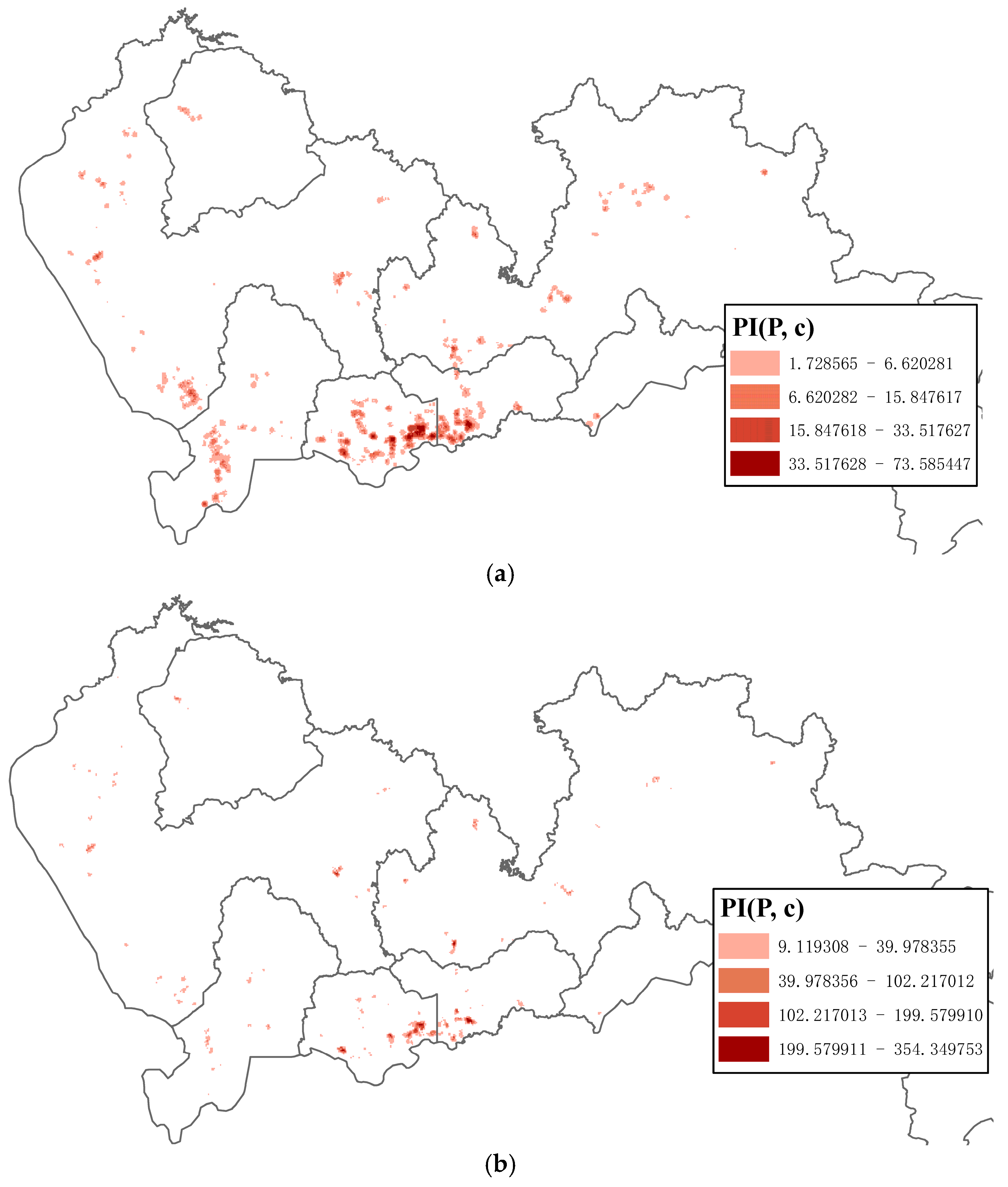
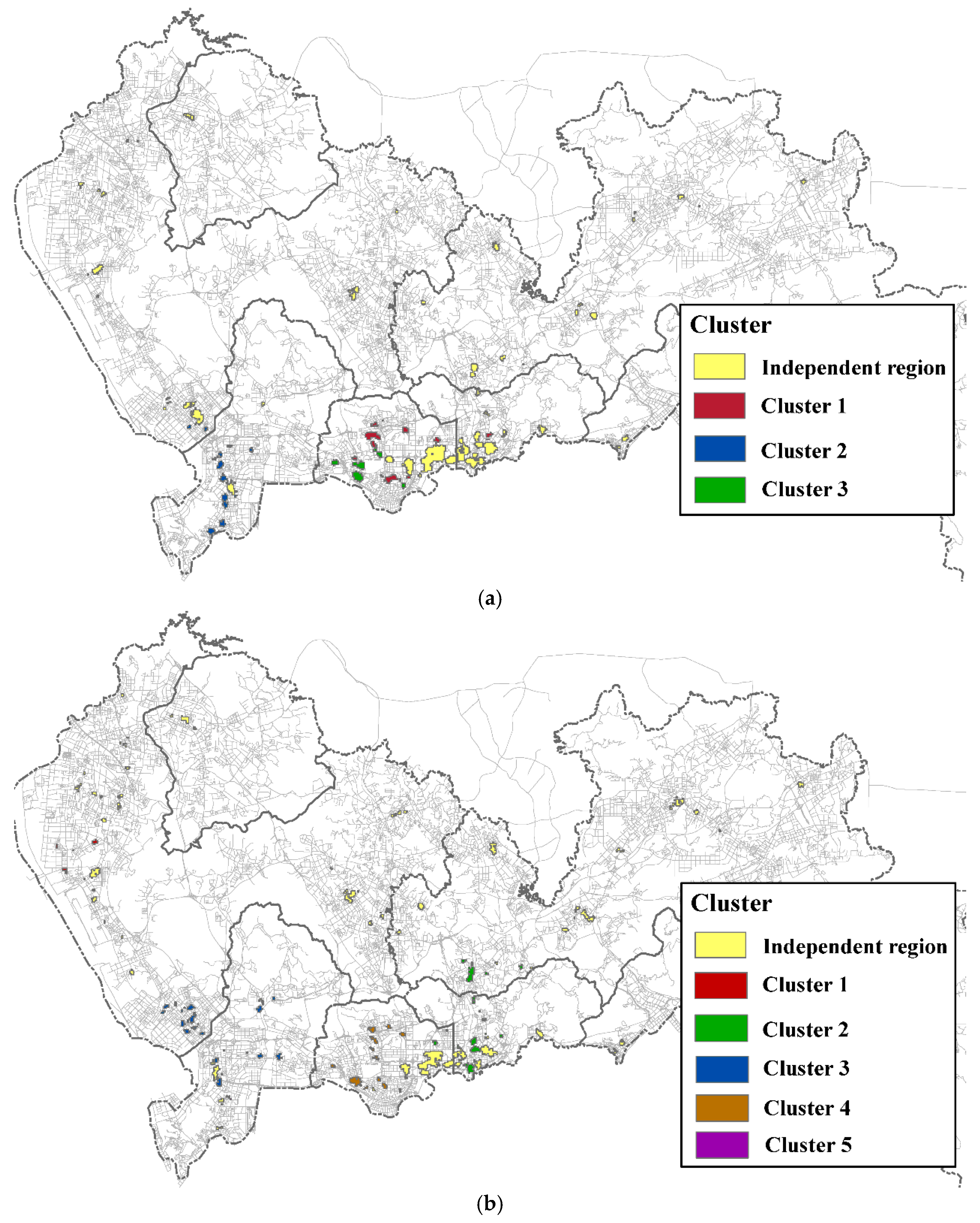
Measure pair-wise similarity between the polygons by considering both the location-based and contextual variables, and subsequently employing a density-based clustering algorithm to cluster the polygons to create a classification of prevalent regions (Section 2.4).

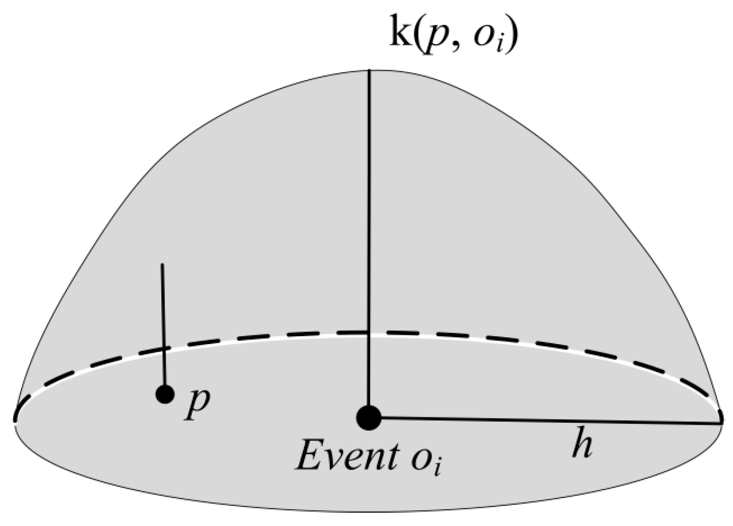
2.2. Generating KDE Surfaces for Point Features

There are two common methods to estimate the spatial density of events across space, namely quadrat counting and KDE. The quadrat counting method divides the entire region into a certain number of cells and counts separately the number of events that fall within each cell to calculate the individual cell density values. Selection of the quadrat size affects the resulting density surface. The counting method does not consider the spatial relationships across the selected quadrat boundaries, and thus it may underestimate the intensity of event distributions if the quadrat size is decreased. It may also disregard some detailed information if the quadrat size is large. The reasons of choosing KDE method for co-location analysis exist in: (1) KDE method can model the spread of influence of an event by defining an area around the event where there is an increased possibility for an event to occur; and (2) KDE method can use arbitrary and homogenous spatial unit for the entire region which makes surfaces combination and ultimately polygons clustering possible [28,29,30,31].

Specifically, rather than considering the count of events within individual cells, the KDE method places a circular neighborhood around each event point and then applies a mathematical function (i.e., a kernel function) that goes from the highest at the position of the event point to the lowest at the bandwidth boundaries. Figure 2 presents an illustration where the kernel value k(p, o_i) decreases with the increase of distance from the ith observation point o to the measuring location p. If the measuring location falls within the neighborhood of multiple observation points, KDE method sums these individual kernel values for that measuring location. Kernel density at location p is estimated as:

$$g\left(p\right)=\frac{1}{n{h}^2}{\displaystyle \sum }_{i=1}^n\mathrm{k}\left(p,o_i\right)$$

(2)

where n is the number of event points, and h is the bandwidth or distance decay threshold.

The kernel function k(p, o_i) can take different forms such as Gaussian, Quartic, Conic, etc. It is widely recognized that the choice of kernel function does not influence density estimation results significantly [29,31]. In this respect, this study use Quartic function, one of the most common kernel functions, for our case study. In addition, the effect of using KDE for point datasets is to produce a smooth and continuous surface. The size of bandwidth can affect the resulting density surface. For example the larger the bandwidth the smoother the surface will be. The literature review presents that the choice of bandwidth is somewhat subjective [28,29,31]. The final choice should be adjusted according to the condition of experimental datasets. We will explain in detail our settings in Section 3.2.

2.3. Combining KDE Surfaces and Identifying Prevalent Regions of a Pattern

Step 1 generates multiple surfaces whereby the grid cell attribute represents the intensity of events of different types. These grid surfaces provide the basis for evaluating the probability that different features co-occur within individual cells. To be part of a prevalent region of a co-location pattern, a grid cell has to have a high event density level on all the surfaces evolved. In this way, the results are the prevalent regions where the pattern prevalence is at its most intense.

Figure 3 shows the combining process of multiple KDE surfaces. Firstly, the grid cells which have a high density attribute value for all the features are selected (see the green and red coloring cells in Figure 3b). Then, a high prevalence measure value is calculated for the selected cells on the final surface (see the yellow coloring cells in Figure 3c), by implementing the local measure PI(P, c) as following:

$$\mathrm{PI}\left(P,c\right)={\displaystyle \prod }_{f\in P}g\left(c\right)$$

(3)

where P and c are the co-location pattern and the cell under investigation, respectively. The prevalence measure is calculated as the product of event density estimations of different features. Based on this measure, a prevalent location (or cell) is expected to have a high probability PI(P, c) of the pattern occurring within the cell.

After creating the prevalence surface, it is possible to select all the prevalent cells for the pattern of interest by specifying a prevalence measure threshold. Prevalent regions are formed by the merging of neighboring cells. A prevalent region could consist of one single cell or multiple cells. Only the cells that share one side can be merged together. With iterative merging, each prevalent cell would be part of a prevalent region, and all the prevalent regions are stored in spatial database as polygons. Most of the previous co-location mining approaches present results in a textual format or non-spatial representation [3,4,24,32]. As a comparison, the main objectives of this research are to maintain the location related information of original data, and establish a basis for the further analysis of the causes of pattern with environmental variables (see Section 2.4).

2.4. Polygon Dissimilarity Function and Clustering

In this section, we propose a spatial clustering method to classify multiple polygons that have hidden relations both in location-based and environmental aspects. As demonstrated in Section 2.3, the input polygons for clustering algorithm are created on the surface of co-location prevalence measure. Therefore, in order to extract similar groups from polygon dataset, the potential cause(s) that spatial features co-occur within a local area should be firstly identified. Specifically, the reasons that a co-location pattern occurs in different regions mainly lie in two aspects: (1) spatial interactions are usually influenced by the geometric distance between objects, and thus the pattern existing within near regions are more possible to be due to common cause(s) than those within farther regions; and (2) in different regions, a pattern is usually formed due to different environmental factors, not just to the co-located features themselves. For example, as shown in Figure 4, urban facilities may be located together to achieve benefits from the agglomeration effects of services (the lower-left block in Figure 4) [33]. This local pattern is due to the spatial interactions between the features themselves. It should be noted that environmental factors such as street network accessibility or government involvement also have a large influence on the selection of facility sites (the upper-right block in Figure 4). Urban environment is a special compact space in which many embedded facilities are constrained to the spatial alignment of street network for reducing transport cost [5,6]. In this respect, co-location pattern between facilities existing within different regions may be due to their own characteristics or to the constraint of street network accessibility. We need to discriminate the “real” prevalent regions influenced by the underlying spatial features from the others influenced by environmental conditions.

Therefore, this section proposes a polygon dissimilarity function that integrates the location-based and environmental variables to accurately classify the prevalent regions of a pattern of interest. The details are as follows:

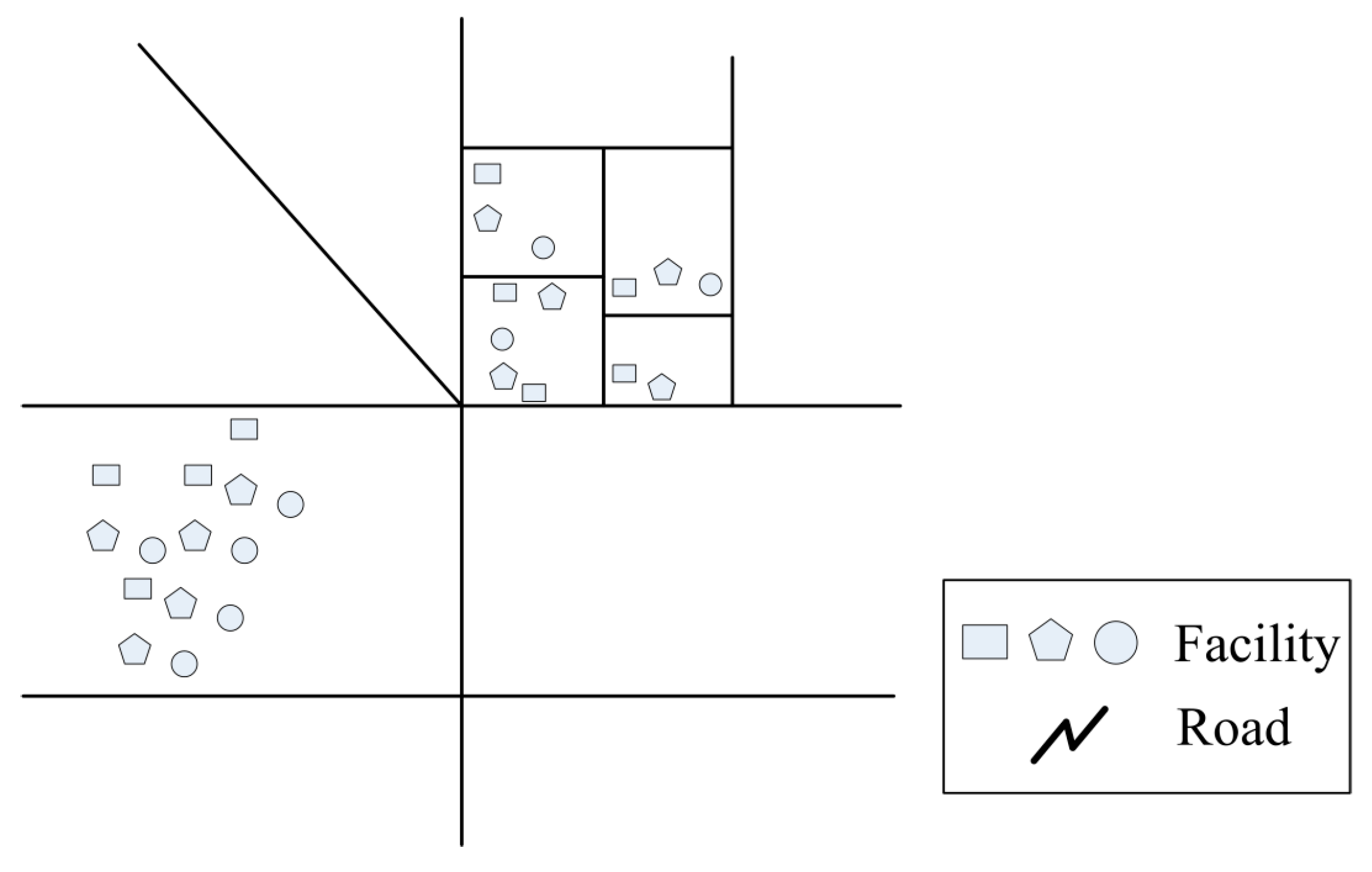
(a)

First, the distance between polygons can be measured by different functions including centroid, separation, min-max, and Hausdorff distance functions [25,26]. Among them, Hausdorff distance is defined as the maximum distance of a point in one set to the nearest point in the other set. Hausdorff distance is appropriate for measuring spatial relations between two polygons due to its adaptability to concave polygons [25]. In this respect, we choose the Hausdorff distance function for our method to accurately measure the geometric distance between two prevalent regions. The mathematical formalization of the Hausdorff distance for two given point sets A and B is defined as

$${\mathrm{D}}_{\mathrm{H}}\left(A,B\right)=\max \left\{{\max }_{a\in A}\left\{{\min }_{b\in B}\mathrm{d}\left(a,b\right)\right\},{\max }_{b\in B}\left\{{\min }_{a\in A}\mathrm{d}\left(a,b\right)\right\}\right\}$$

(4)

where d(a, b) is usually taken as the Euclidean distance between points a and b. For simplicity, we use all the vertices on the polygon boundaries to estimate the Hausdorff distance between two polygons.

(b)

Second, domain experts usually intend to identify a group of regions from spatial database which are not only similar in their spatial locations, but also share one or several common environmental variable(s). Dissimilarity function based on this condition is different from generic functions used by previous clustering methods [34]. To comprehensively understand co-location patterns across different regions, we cluster all the prevalent polygons by considering their environmental variables related to the pattern, e.g., the underlying street network accessibility and the government facility density. Given two polygons A and B and their associated environmental variables {v_A1, v_A2, …, v_An} and {v_B1, v_B2, …, v_Bn}, we can measure their contextual distance using the standard Euclidean distance function as following.

$${\mathrm{D}}_{\mathrm{C}}\left(A,B\right)=\sqrt{{\displaystyle \sum }_{i=1}^n{\left(v_{Ai}-v_{Bi}\right)}^2}$$

(5)

where all the environmental attributes v_Ai and v_Bi are normalized for integration. Furthermore, we can also assign different weights to the various variables according to the interest of domains. Our study chooses equal weights for simplicity.

Based on the above distance functions, we use a weighted sum of the Hausdorff distance and the contextual distance to define polygon dissimilarity function as following.

$${\mathrm{D}}_{\mathrm{Polygon}}\left(A,B\right)=w_H{\mathrm{D}}_H\left(A,B\right)+w_C{\mathrm{D}}_C\left(A,B\right)$$

(6)

where $w_H$ and $w_C$ are the weights associated with the Hausdorff distance and the contextual distance, respectively, and $w_H$ + $w_C$ = 1 ($w_H>0 \mathrm{and} w_C>0$). The two weights should be adjusted according to the contributions of location-based and environmental variables for a prevalent region. Based on the polygon dissimilarity function, we can measure the degree of similarity between any two prevalent regions with respect to the pattern of interest. The proposed method stores the result with a dissimilarity matrix; if there is k polygons, the size of matrix would be k × k. In this way, standard spatial clustering algorithms (e.g., density-based clustering, partitional clustering, etc.) can be used with this matrix for classifying prevalent regions. We choose DBSCAN (Density-Based Spatial Clustering of Applications with Noise) algorithm as it does not need to predefine the number of clusters and is able to discover clusters of arbitrary shapes [33]. Actually, other improved clustering and co-clustering methods can also be used in our framework [35,36,37]. This occurs because the key component of the proposed framework is the calculation of polygon dissimilarity matrix, and it does not restrict the following subtask using other improved clustering algorithms (e.g., the Shared Nearest Neighbor algorithm and HOCCLUS2 biclustering algorithm). In addition, the use of a generic clustering algorithm (e.g., DBSCAN algorithm) enables users to more easily re-implement the proposed framework.

Our approach extends traditional ones by introducing polygons clustering algorithm. Thus, the performance of the proposed algorithm largely depends on the computational complexity in polygons clustering. Computing the dissimilarity matrix needs to measure the pair-wise dissimilarity between all the polygons with respect to the concerned variables. Thus, its computational complexity will be O(k × k × n), where k is the number of prevalent regions and n the total number of location-based and environmental variables. In addition, the computational complexity of DBSCAN algorithm is O(k log k) [33]. Based on the above, the polygons clustering algorithm has the complexity of O(k × k × n) + O(k log k), which is higher than the traditional algorithms that do not need to cluster the prevalent regions. The traditional algorithms only focus on the step related to the delimitating of prevalent regions, and lack attention to the analysis of the similarity between the prevalent regions. Therefore, although the proposed algorithm costs more time, it can find more in-depth information by generating and clustering the prevalent regions.

3. Experiments

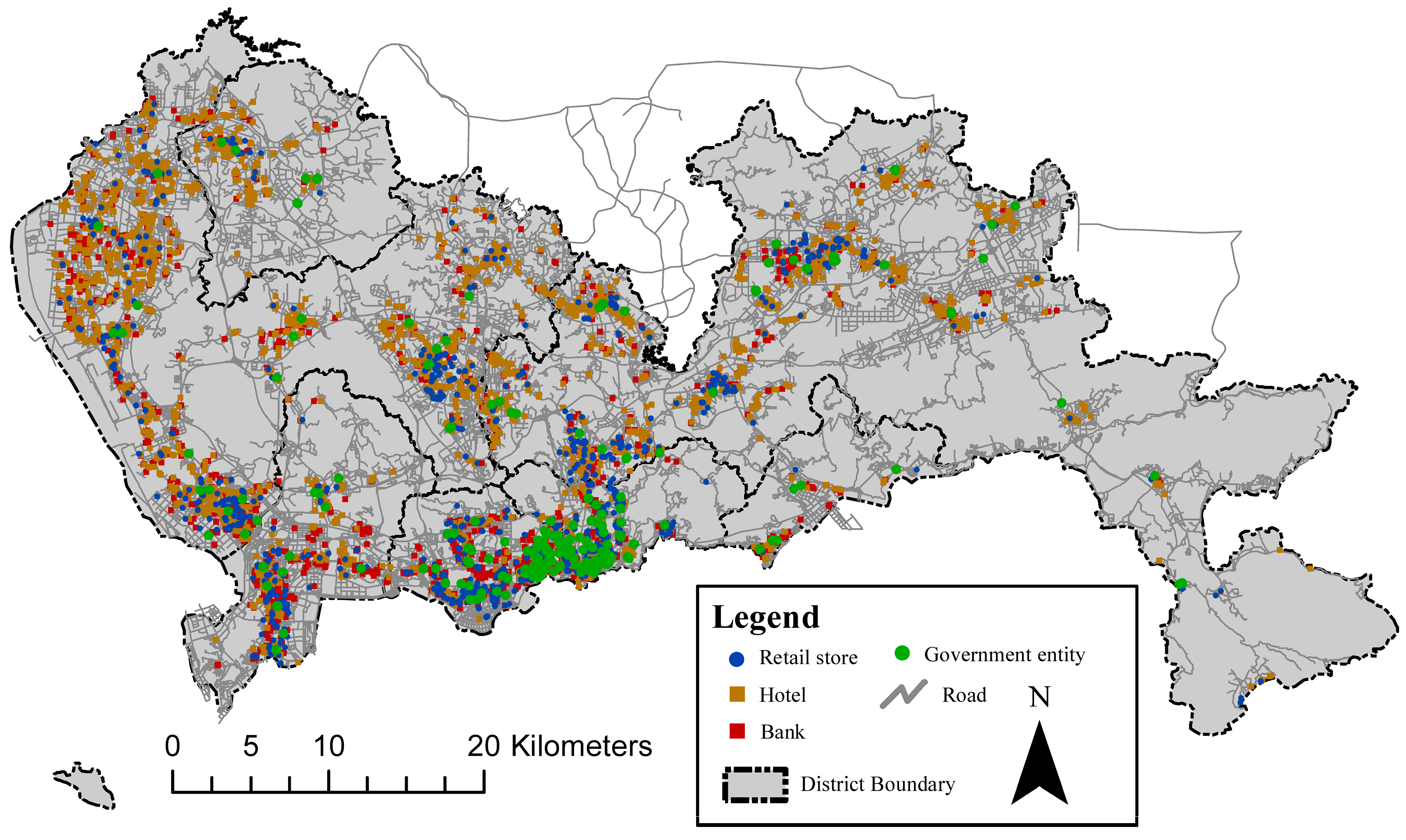
3.1. Data

In order to evaluate our method, we used urban facility points-of-interest (POIs) of Shenzhen, China, for scoping co-location patterns and clustering their prevalent regions with additional environmental datasets of street network and government entities (Figure 5). There are three POI features participating in the co-location mining, including bank, hotel and retail store. Features bank, hotel and retail store have 1654, 3128 and 888 points, respectively. The reason that we chose urban facility datasets is due to their implications in regional structure of urban services and functions. For example, facilities bank, hotel and retail store correspond to the financial function, accommodation function and retail function of an urban system, respectively. Spatial interactions between contiguous urban services exist within specific regions, e.g., central business district. Therefore, identifying their prevalent regions can help urban planners and managers comprehensively understand the urban system and formulate reasonable policy to improve the urban environment.

As presented in Section 2.4, the proposed method takes into account the environmental factors that could influence the prevalence of a co-location pattern in local regions. In this respect, our experiments used two additional datasets including the street network dataset and the government entity POIs dataset. Specifically, the spatial density of street network within individual prevalent regions was used to indicate the accessibility of the corresponding region, and the density of government entity POIs was used to indicate how much the local co-location pattern is affected by the governmental inference. The street network consists of 37,932 network segments, and the number of government entity POIs is 394.

3.2. Setting

We divided the Shenzhen area into a 750 × 367 grid with 100-m cell size. Since the study city covers an approximate area of 2752 km², the cell granularity is fine enough to capture the local information of the experimental datasets. Based on the grid, the KDE function (Equation (2)) is computed for each feature using a bandwidth of 300 m. As discussed in Section 2.2, there is no universal rule for determining the bandwidth of KDE, and thus this case study chose the bandwidth according to the suggestions of scholars [38,39], i.e., a 100–300 m bandwidth is appropriate for analyzing spatial interactions at the neighborhood scale. Our study region covers the whole metropolitan area of Shenzhen, and thus we chose the maximum parameter (i.e., 300-m bandwidth) in the interval. Furthermore, we also used a larger parameter (i.e., 600 m) to comprehensively evaluate the proposed method (see Section 3.4). The prevalence threshold for creating prevalent polygons is set to 5, which is about equal to the tail value boundary of the entire prevalence surface using two positive standard deviations. For the polygon dissimilarity function, both the weight factors were set to 0.5 for balancing the contributions of location-based variable and environmental variable. DBSCAN clustering algorithm requires two parameters, i.e., the radius ε and the minimum number of polygons minPolys, to form a dense cluster [34]. In our experiments, ε and minPolys were set to 0.06 and 5, respectively. Furthermore, we also used different parameter settings to examine the effectiveness of the proposed approach.

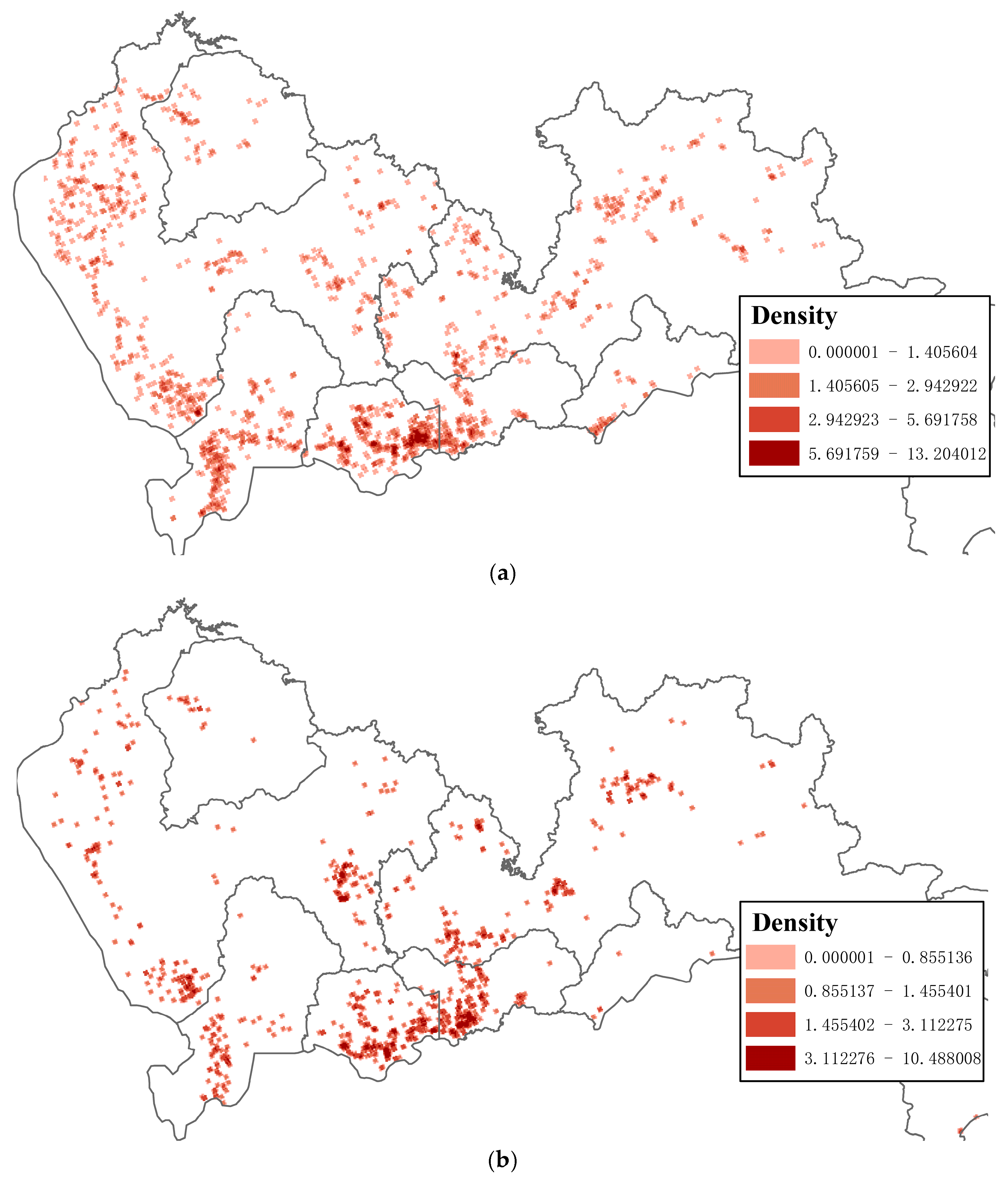
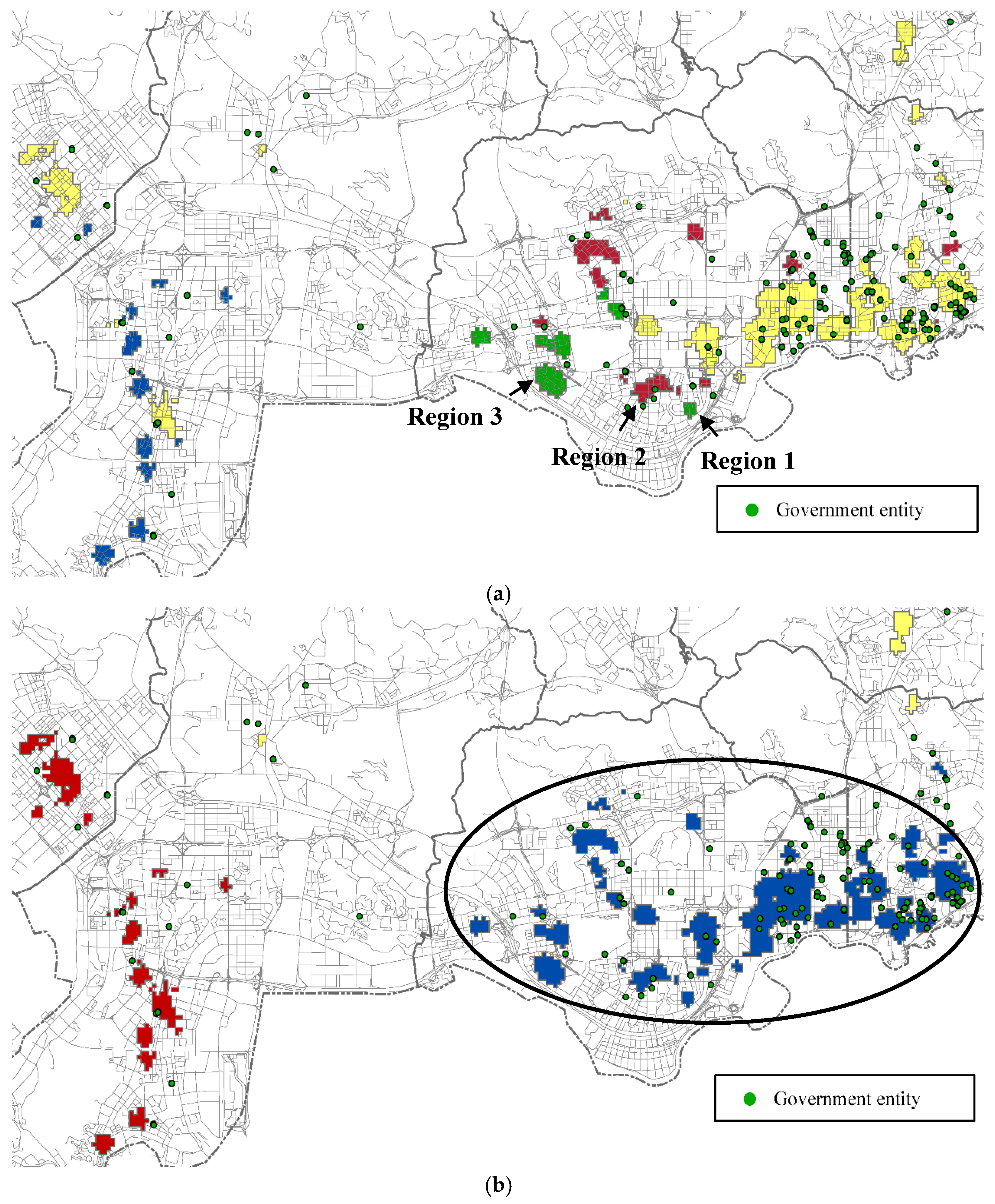
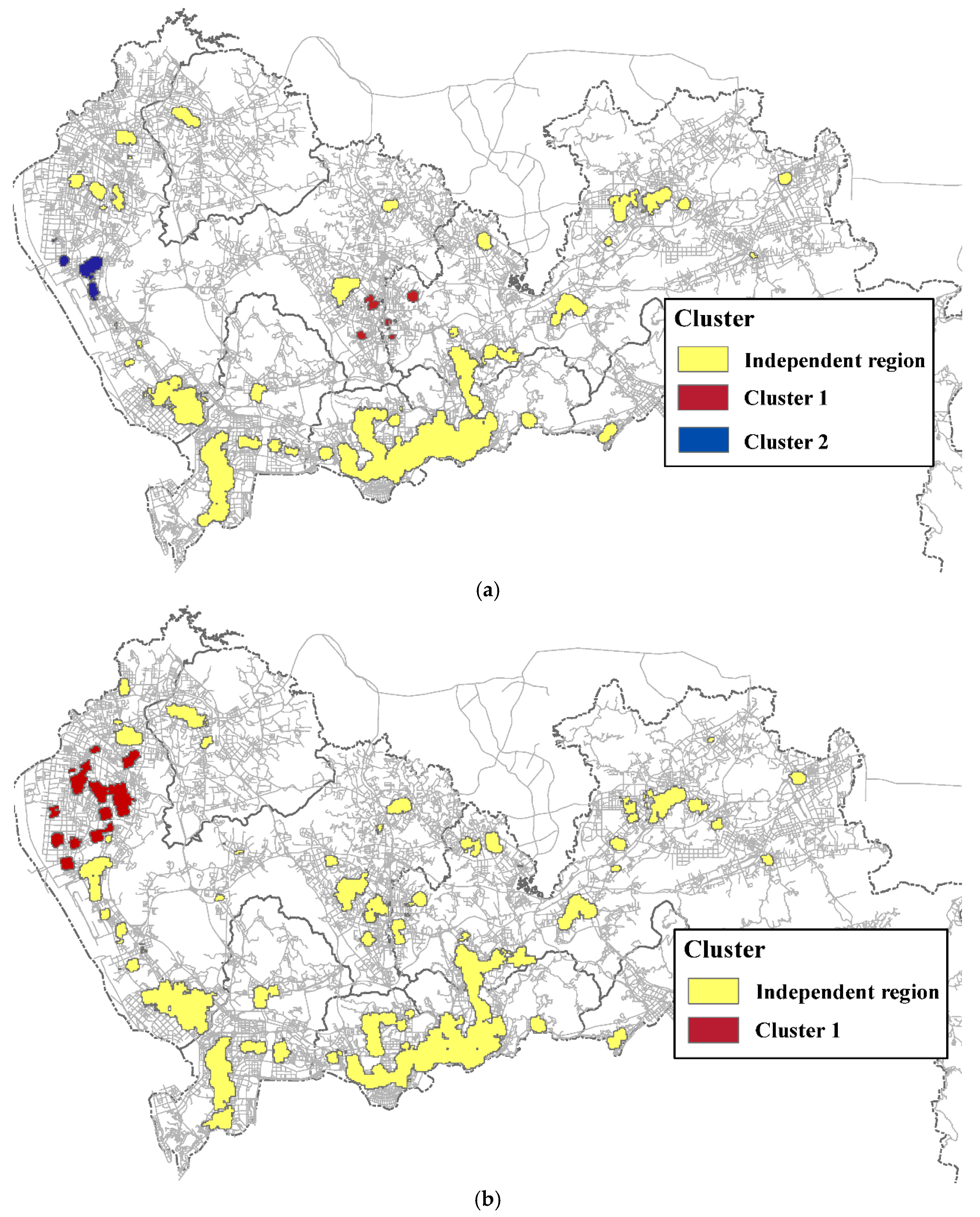
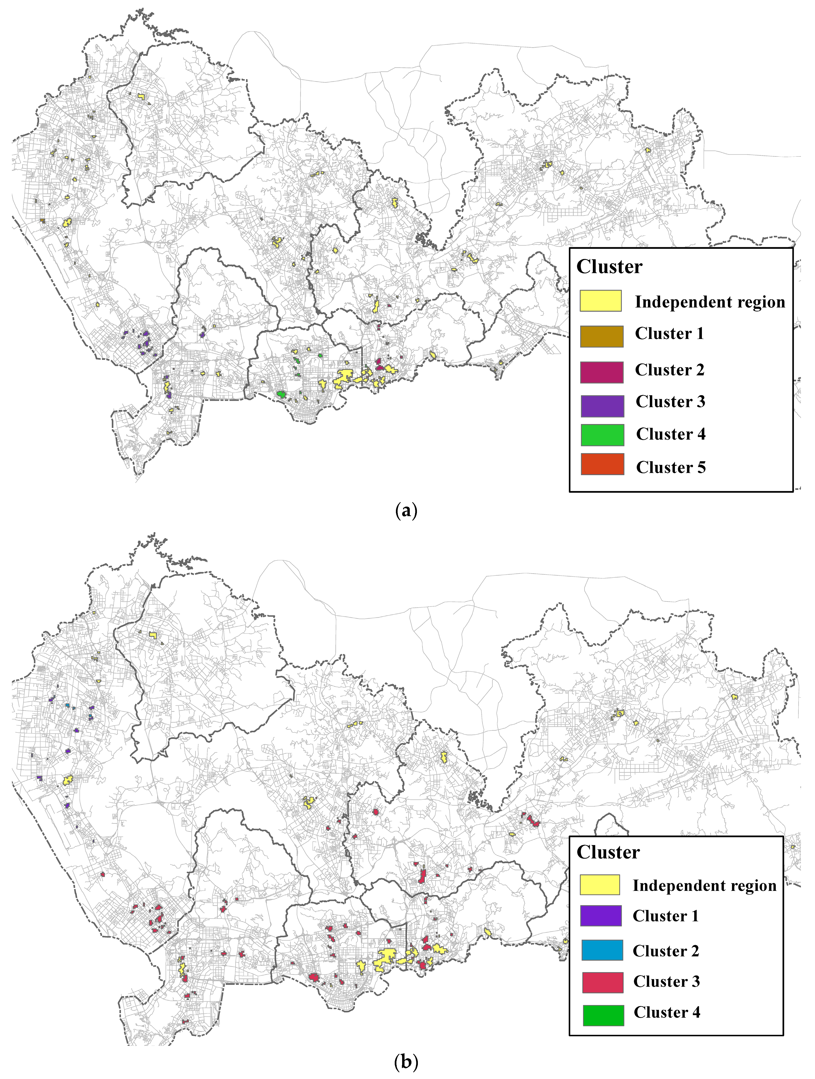
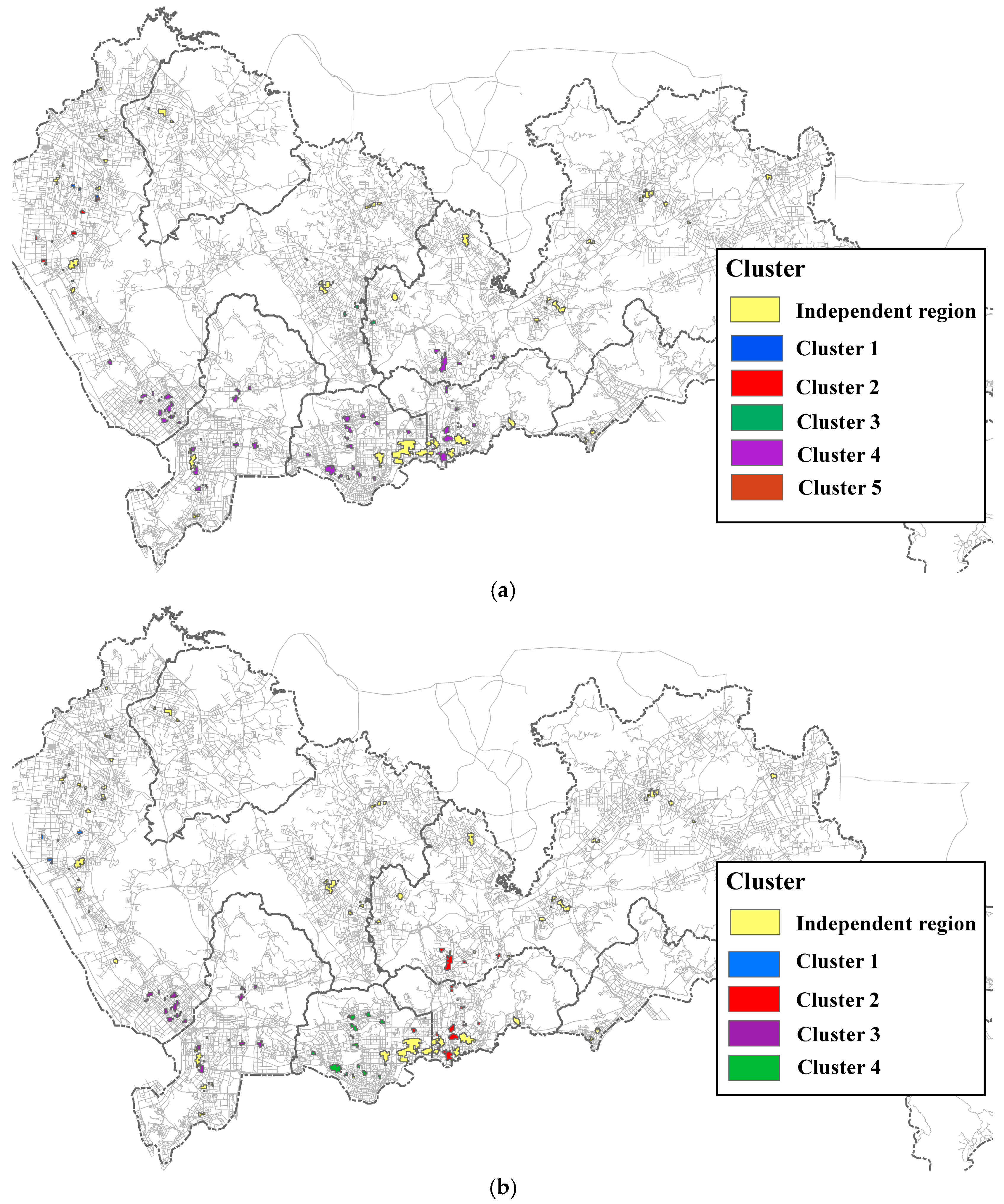
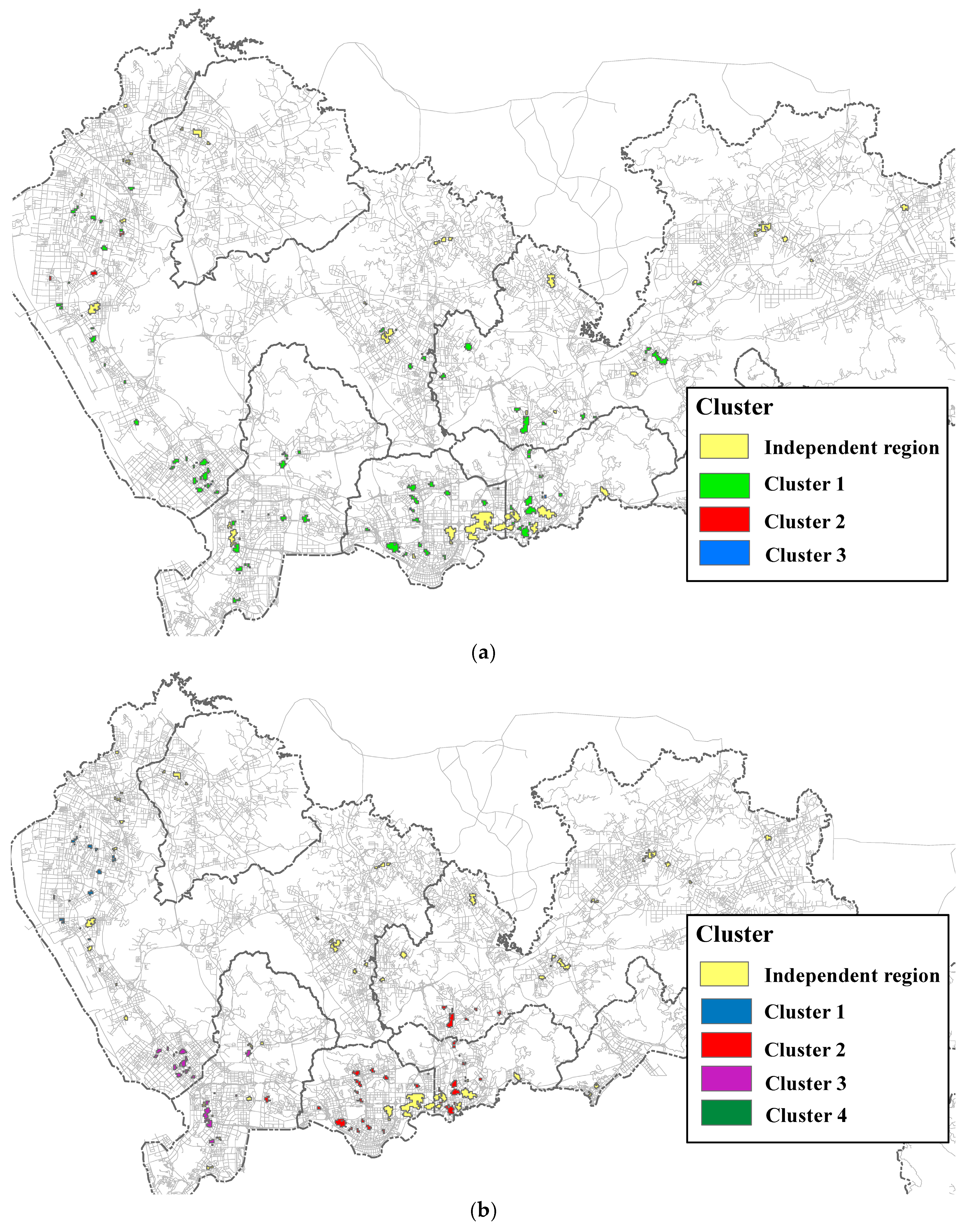
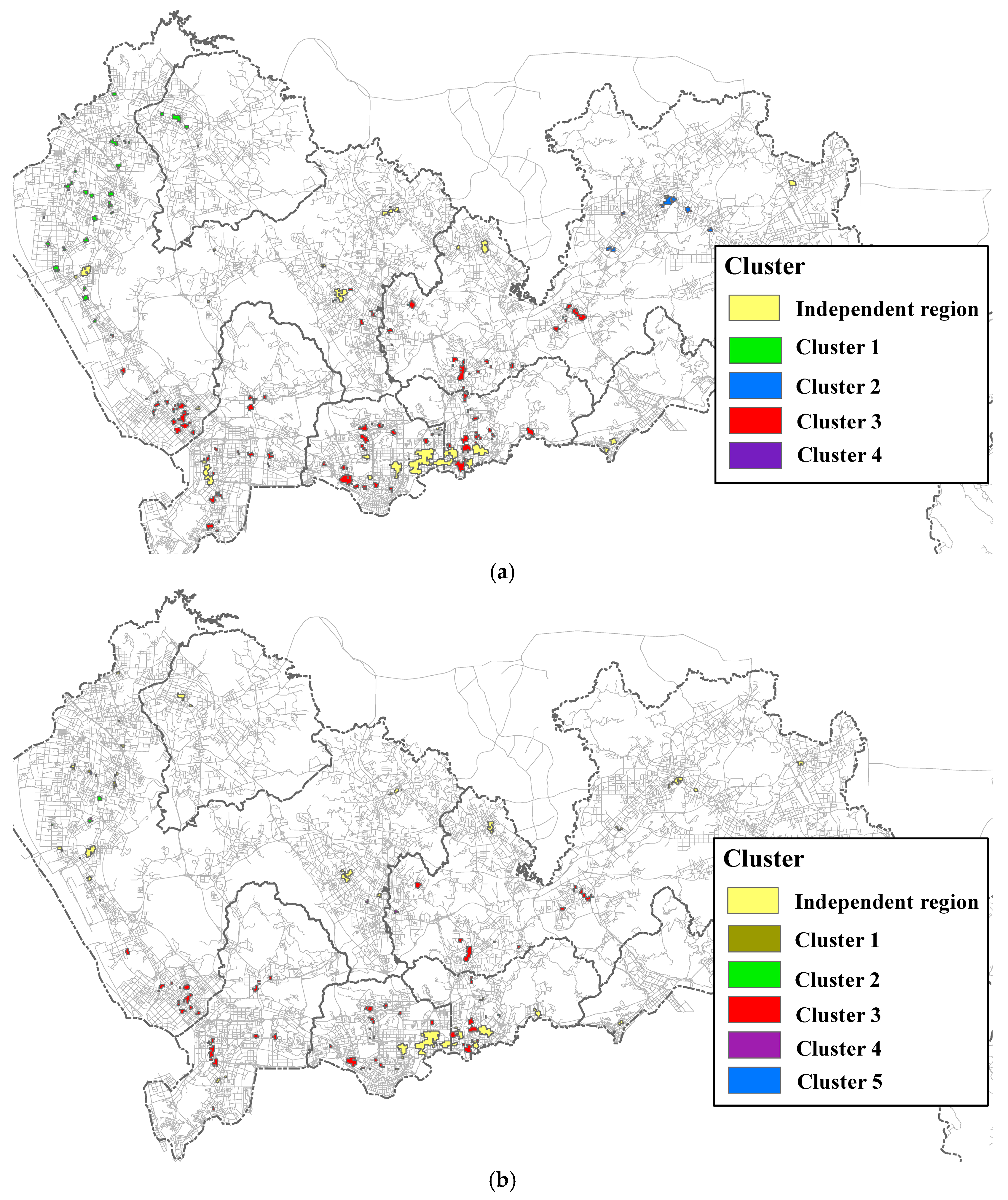
3.3. Results and Analysis

Generally, by representing the intensity distributions of POIs using KDE surfaces, one can identify simple and intuitive spatial patterns of individual urban services in the study region, e.g., “hot spots” and “cold spots”. As shown in Figure 6, the spatial distributions of Shenzhen’s financial, accommodation and retail services are largely consistent across most districts. Some regions exhibit a co-location pattern with different prevalence level. For example, the western region in Shenzhen has a high density value of financial services but a low density value of retail services. Therefore, to provide some interesting association information, we further created two co-location prevalence surfaces from the KDE surfaces using the prevalence measure PI(P, c) as defined in Equation (3). The combined surfaces with respect to the size-2 pattern {bank, retail store} and the size-3 pattern {bank, retail store, hotel} are presented in Figure 7.

As shown in Figure 7, the surfaces present the spatial variations of prevalence of the two patterns. Specifically, by identifying the surface peaks in Figure 7a, facilities bank and retail store are frequently co-located within the southern, southwestern and northwestern regions. In addition, the surface peaks in Figure 7b indicate that facilities bank, retail store and hotel have a strong dependency relationship in the southern region of Shenzhen. The area of the surface peaks in Figure 7b is shrunk compared to those in Figure 7a.

Next, we generated prevalent polygons from the prevalence surfaces in which the prevalence measure value is above a certain threshold (i.e., 5). As presented in Figure 8, these polygons represent prevalent regions of the pattern in which all the urban services evolved are concentrated above a certain level. The numbers of the polygons in Figure 8a,b are 20 and 30, respectively. In this way, it is intuitive to capture the range and extent of the patterns of interest. Under the research background of this study, further analysis can be done to help urban managers implement the policy zoning of urban system.

Furthermore, we calculated the dissimilarity function between all the pairs of the polygons. There are two types of dissimilarity functions for our case: i.e., the simple function based solely on the Hausdorff distance and the hybrid function based on both the Hausdorff distance and the contextual distance. The contextual distance is based on the factor that contextual environment has an important role in the formation of co-location patterns in local areas. For our case study, the contextual distance is measured using the street network accessibility and the government facility density. More specifically, the street network accessibility in each region is calculated by dividing the total length of the street segments fallen within the region by the area of the polygon. The government facility density in each region is calculated by dividing the total number of the government facility POIs fallen within the region by the area of the polygon. Based on the two indicators, we then integrated the hybrid dissimilarity function into the standard DBSCAN algorithm. As shown in Figure 9, the final clustering results can be utilized to summarize what characteristics the prevalent regions in the same groups share.

We further implemented the DBSCAN algorithm based on the simple dissimilarity function to demonstrate the effectiveness of our approach. Specifically, as presented in a zoom-in portion of the results using the simple dissimilarity function and the hybrid dissimilarity function (Figure 10), we can find that the clusters vary greatly with different functions. For example, polygons highlighted by the circle in Figure 10b are clustered as the same group due to their near locations, while by incorporating the contextual factors most of them are identified as belonging to different groups (Figure 10a). The clustering result as shown in Figure 10b comes from the simple awareness of the common cause(s) existing between near regions or patterns. However, the accessibility constraint and governmental inference usually have a great influence in promoting the co-location of urban services in local regions, even if these regions are distributed in distant places. For example, as presented in Figure 10a, although Region 2 is closer to Region 1 than Region 3, our approach identifies Regions 1 and 3 as belonging to the same cluster (i.e., Cluster 3) and Region 2 as belonging to Cluster 1. Therefore, the proposed method, which considers the location-based and contextual variables, is very helpful for domain experts to identify the causes that result in the spatial heterogeneity of a co-location pattern.

3.4. Effects of Parameter

In the next experiment, we evaluated the effectiveness of the proposed approach with a larger parameter (i.e., 600-m bandwidth). Other parameters are the same as in the previous experiments. Since a larger bandwidth will produce a smoother KDE surface for individual features, the combined prevalence surface with respect to the pattern of interest could achieve an increasing smooth characteristic with the increase of bandwidth. In this respect, the prevalent regions identified with a larger bandwidth are more wide-ranging, and the clustering algorithm creates a larger agglomeration with the merging of neighboring polygons (Figure 11).

Secondly, we evaluated the effect of different radiuses in the DBSCAN algorithm. As shown in Figure 12, with the increase in radius, a neighborhood area becomes larger and the number of clusters decreases. The size of clusters also increases with increase of the radius. We can observe that the polygons in Shenzhen’s southern area are merged into a single cluster in Figure 12b. Thus, the parameter of radius should be carefully designed according to the spatial scale of applications. For example, the district-level planning could choose a larger radius and the subdistrict-level planning could choose a smaller parameter.

Then, we compared the effect of the minimum number of polygons in the DBSCAN algorithm. The increase of minimum number of polygons makes the ε-neighborhood harder to be “dense” and decreases the number of core polygons (or clusters). As shown in Figure 13, polygons tend to form small-sized clusters with increase of the minimum number of polygons.

Next, we evaluated the effect of the weight of distances in the algorithm. When the weight $w_C$ is larger than $w_H$, the contribution of environmental variables is larger than that of location-based variable (please see Equation (6)). As shown in Figure 14a, most of the polygons in the city are grouped into a single cluster, even though some polygons are distributed in remote regions. This occurs because a small weight of $w_H$ can weaken the effect of the location-based variable in polygons clustering, and most of the polygons in the city have a similar environmental variable. In contrast, when the weight $w_C$ is smaller than $w_H$, nearby polygons are more likely to form a cluster (Figure 14b).

In addition, we examined the influence of different prevalence thresholds (PI) on the final result. As shown in Figure 15, the increase of PI threshold makes prevalent regions less and increases the number of clusters. The larger PI threshold leads to a higher concentration of features. Thus, the delimitated areas by a higher threshold could better express the pattern’s prevalence.

Finally, although our experiments only considered two contextual variables in the polygons clustering approach, any other variables (e.g., population density) associated with urban service patterns can also be integrated into the polygon dissimilarity function to provide a more comprehensive tool for domain experts. The choice of contextual variables should be adjusted according to the interest of domain experts.

4. Conclusions and Outlook

Traditional spatial co-location pattern mining approaches are useful to identify universal spatial relations existing in the whole study region by outputting the results in a textual format. This paper has proposed a novel approach for identifying and classifying the prevalent regions of a co-location pattern with a particular focus on the spatial heterogeneity property of spatial interactions. The main contributions of this paper are summarized as follows.

(1)

Firstly, this paper proposed a new polygon clustering framework for delimitating and classifying the prevalent regions of a co-location pattern.

(2)

Secondly, Polygons generated by combining multiple KDE surfaces give the prevalent regions of the pattern of interest, which may be pruned in traditional approaches because of its low prevalence measure value at the global scale. In this way, we can capture some valuable information hidden within a local area.

(3)

Thirdly, the addition of environmental datasets provides us a more comprehensive means of classifying the prevalent regions not only from geometric distance perspective but also from contextual perspective. A polygon dissimilarity function based on Hausdorff distance and contextual distance is integrated into the clustering algorithm to identify similar prevalent regions of a pattern that may be formed by several common cause(s). In this way, we can identify whether a local co-location pattern is formed by the features themselves or by their contextual environments (e.g., accessibility).

The proposed approach was applied to the analysis of co-location patterns of urban services. We could delimitate the prevalent regions of the patterns of urban services, and extract the groups of these regions by considering location-based and contextual factors that are usually ignored by existing approaches. The key idea of our study is to expand the existing framework to investigate interesting regions in which multiple features are frequently co-located due to their own spatial interactions or the environmental factors. Our method is an alternative from the co-location mining with rare features [40] to resolve pattern loss.

The study offers several interesting areas for further research. For example, as shown in Figure 3, we can define and represent the combining process of KDE surfaces using the RGB color model where red stands for feature B, green stands for feature A. In this way, each cell is assigned a triple (red-value, green-value, blue-value) according to the density estimation of events of different features within the cell. For example, in Figure 3, the cells with high density values of feature A and feature B get a high yellow value according to the RGB model theory of “Red + Blue = Yellow”. Finally, with the increasing collection of large volumes of spatial datasets, our future work will test the proposed approach under different domain applications. For example, it is interesting to investigate the reasons that ecological species are frequently co-located within several local areas, instead of the entire region.

References

- Bogorny, V.; Kuijpers, B.; Alvares, L. Reducing uninteresting spatial association rules in geographic databases using background knowledge: A summary of results. Int. J. Geogr. Inf. Sci. 2008, 22, 361–386. [Google Scholar] [CrossRef]
- Flouvat, F.; Van Soc, J.F.N.; Desmier, E.; Selmaoui-Folcher, N. Domain-driven co-location mining. GeoInformatica 2015, 19, 147–183. [Google Scholar] [CrossRef]
- Shekhar, S.; Huang, Y. Discovering spatial co-location patterns: A summary of results. In Proceedings of the 7th International Symposium, SSTD 2001, Redondo Beach, CA, USA, 12–15 July 2001. [Google Scholar]
- Huang, Y.; Shekhar, S.; Xiong, H. Discovering colocation patterns from spatial data sets: A general approach. IEEE Trans. Knowl. Data Eng. 2004, 16, 1472–1485. [Google Scholar] [CrossRef]
- Yu, W. Spatial co-location pattern mining for location-based services in road networks. Expert Syst. Appl. 2016, 46, 324–335. [Google Scholar] [CrossRef]
- Yu, W.; Ai, T.; He, Y.; Shao, S. Spatial co-location pattern mining of facility points-of-interest improved by network neighborhood and distance decay effects. Int. J. Geogr. Inf. Sci. 2017, 31, 280–296. [Google Scholar] [CrossRef]
- Ding, W.; Eick, C.F.; Yuan, X.; Wang, J.; Nicot, J.P. On regional association rule scoping. In Proceedings of the International Workshop on Spatial and Spatio-Temporal Data Mining, Omaha, NE, USA, 28–31 October 2007. [Google Scholar]
- Ding, W.; Eick, C.F.; Yuan, X.; Wang, J.; Nicot, J.P. A framework for regional association rule mining and scoping in spatial datasets. GeoInformatica 2011, 15, 1–28. [Google Scholar] [CrossRef]
- Mennis, J.L.; Guo, D. Spatial data mining and geographic knowledge discovery—An introduction. Comput. Environ. Urban Syst. 2009, 33, 403–408. [Google Scholar] [CrossRef]
- Shekhar, S.; Chawla, S. Spatial Databases: A Tour; Prentice Hall: Upper Saddle River, NJ, USA, 2003. [Google Scholar]
- Akbari, M.; Samadzadegan, F.; Weibel, R. A generic regional spatio-temporal co-occurrence pattern mining model: A case study for air pollution. J. Geogr. Syst. 2015, 17, 249–274. [Google Scholar] [CrossRef]
- Li, J.; Adilmagambetov, A.; Jabbar, M.S.M.; Zaïane, O.R.; Osornio-Vargas, A.; Wine, O. On discovering co-location patterns in datasets: A case study of pollutants and child cancers. GeoInformatica 2016, 20, 651–692. [Google Scholar] [CrossRef]
- Mennis, J.L.; Liu, J.W. Mining association rules in spatio-temporal data: An analysis of urban socioeconomic and land cover change. Trans. GIS 2005, 9, 5–17. [Google Scholar] [CrossRef]
- Agrawal, R.; Srikant, R. Fast algorithms for mining association rules. In Proceedings of the 20th International Conference on Very Large Data Bases (VLDB), Santiago, Chile, 12–15 September 1994. [Google Scholar]
- Koperski, K.; Han, J. Discovery of spatial association rules in geographic information databases. In Advances in Spatial Databases; Springer: Berlin/Heidelberg, Germany, 1995; pp. 47–66. [Google Scholar]
- Tobler, W.R. A computer movie simulating urban growth in the Detroit Region. Econ. Geogr. 1970, 46, 234–240. [Google Scholar] [CrossRef]
- Getis, A.; Ord, J.K. The analysis of spatial association by use of distance statistics. Geogr. Anal. 1992, 24, 189–206. [Google Scholar] [CrossRef]
- Openshaw, S. Developing automated and smart spatial pattern exploration tools for geographical information systems applications. Statistician 1995, 44, 3–16. [Google Scholar] [CrossRef]
- Bembenik, R.; Rybinski, H. FARICS: A method of mining spatial association rules and collocations using clustering and Delaunay diagrams. J. Intell. Inf. Syst. 2009, 33, 41–64. [Google Scholar] [CrossRef]
- Sierra, R.; Stephens, C.R. Exploratory analysis of the interrelations between co-located boolean spatial features using network graphs. Int. J. Geogr. Inf. Sci. 2012, 26, 441–468. [Google Scholar] [CrossRef]
- Leslie, T.F.; Kronenfeld, B.J. The colocation quotient: A new measure of spatial association between categorical subsets of points. Geogr. Anal. 2011, 43, 306–326. [Google Scholar] [CrossRef]
- Guo, L.; Du, S.H.; Haining, R.; Zhang, L.J. Global and local indicators of spatial association between points and polygons: A study of land use change. Int. J. Appl. Earth Obs. Geoinf. 2013, 21, 384–396. [Google Scholar] [CrossRef]
- Miller, H.J.; Han, J. Geographic Data Mining and Knowledge Discovery; CRC Press: Boca Raton, FL, USA, 2009. [Google Scholar]
- Yoo, J.S.; Shekhar, S. A joinless approach for mining spatial colocation patterns. IEEE Trans. Knowl. Data Eng. 2006, 18, 1323–1337. [Google Scholar]
- Joshi, D.; Soh, L.K.; Samal, A.; Zhang, J. A dissimilarity function for geospatial polygons. Knowl. Inf. Syst. 2014, 41, 153–188. [Google Scholar] [CrossRef]
- Wang, S.; Eick, C.F. A polygon-based clustering and analysis framework for mining spatial datasets. GeoInformatica 2014, 18, 569–594. [Google Scholar] [CrossRef]
- Sengstock, C.; Gertz, M.; Canh, T.V. Spatial Interestingness Measures for Co-location Pattern Mining. In Proceedings of the IEEE 13th International Conference on Data Mining Workshops, Brussels, Belgium, 10 December 2012. [Google Scholar]
- Cressie, N.A.C. Statistics for Spatial Data; John Wiley: Hoboken, NJ, USA, 1991. [Google Scholar]
- Schabenberger, O.; Gotway, C.A. Statistical Methods for Spatial Data Analysis; Chapman Hall/CRC: Boca Raton, FL, USA, 2005. [Google Scholar]
- Yu, W.; Ai, T.; Shao, S. The analysis and delimitation of Central Business District using network kernel density estimation. J. Transp. Geogr. 2015, 45, 32–47. [Google Scholar] [CrossRef]
- O’Sullivan, D.; Unwin., D.J. Geographic Information Analysis; John Wiley: Hoboken, NJ, USA, 2010. [Google Scholar]
- Yoo, J.S.; Bow, M. Mining spatial colocation patterns: A different framework. Data Min. Knowl. Discov. 2012, 24, 159–194. [Google Scholar]
- Monseny, J.; López, R.; Marsal, E. The mechanisms of agglomeration: Evidence from the effect of inter-industry relations on the location of new firms. J. Urban Econ. 2011, 70, 61–74. [Google Scholar] [CrossRef]
- Ester, M.; Kriegel, H.P.; Sander, J.; Xu, X. A density-based algorithm for discovering clusters in large spatial databases with noise. In Proceedings of the Second International Conference on Knowledge Discovery and Data Mining, Portland, OR, USA, 2–4 August 1996. [Google Scholar]
- Ertoz, L.; Steinback, M.; Kumar, V. Finding clusters of different sizes, shapes, and density in noisy high dimensional data. In Proceedings of the 3rd SIAM International Conference on Data Mining, San Francisco, CA, USA, 1–3 May 2003. [Google Scholar]
- Pio, G.; Ceci, M.; D’Elia, D.; Loglisci, C.; Malerba, D. A Novel Biclustering Algorithm for the Discovery of Meaningful Biological Correlations between microRNAs and their Target Genes. BMC Bioinform. 2013, 14, S8. [Google Scholar] [CrossRef] [PubMed]
- Pio, G.; Ceci, M.; Malerba, D.; D’Elia, D. ComiRNet: A Web-based System for the Analysis of miRNA-gene Regulatory Networks. BMC Bioinform. 2015, 16, S7. [Google Scholar] [CrossRef] [PubMed]
- Okabe, A.; Satoh, T.; Sugihara, K. A kernel density estimation method for networks, its computational method and a GIS-based tool. Int. J. Geogr. Inf. Sci. 2009, 23, 7–32. [Google Scholar] [CrossRef]
- Porta, S.; Strano, E.; Iacoviello, V.; Messora, R.; Latora, V.; Cardillo, A.; Wang, F.; Scellato, S. Street centrality and densities of retail and services in Bologna, Italy. Environ. Plan. B Plan. Des. 2009, 36, 450–465. [Google Scholar] [CrossRef]
- Huang, Y.; Pei, J.; Xiong, H. Mining co-location patterns with rare events from spatial data sets. GeoInformatica 2006, 10, 239–260. [Google Scholar] [CrossRef]
© 2017 by the author. Licensee MDPI, Basel, Switzerland. This article is an open access article distributed under the terms and conditions of the Creative Commons Attribution (CC BY) license (http://creativecommons.org/licenses/by/4.0/).
Share and Cite
Yu, W. Identifying and Analyzing the Prevalent Regions of a Co-Location Pattern Using Polygons Clustering Approach. ISPRS Int. J. Geo-Inf. 2017, 6, 259. https://doi.org/10.3390/ijgi6090259
Yu W. Identifying and Analyzing the Prevalent Regions of a Co-Location Pattern Using Polygons Clustering Approach. ISPRS International Journal of Geo-Information. 2017; 6(9):259. https://doi.org/10.3390/ijgi6090259
Chicago/Turabian StyleYu, Wenhao. 2017. "Identifying and Analyzing the Prevalent Regions of a Co-Location Pattern Using Polygons Clustering Approach" ISPRS International Journal of Geo-Information 6, no. 9: 259. https://doi.org/10.3390/ijgi6090259
APA StyleYu, W. (2017). Identifying and Analyzing the Prevalent Regions of a Co-Location Pattern Using Polygons Clustering Approach. ISPRS International Journal of Geo-Information, 6(9), 259. https://doi.org/10.3390/ijgi6090259