Enabling the Use of Sentinel-2 and LiDAR Data for Common Agriculture Policy Funds Assignment

Abstract

A comprehensive strategy combining remote sensing and field data can be helpful for more effective agriculture management. Satellite data are suitable for monitoring large areas over time, while LiDAR provides specific and accurate data on height and relief. Both types of data can be used for calibration and validation purposes, avoiding field visits and saving useful resources. In this paper, we propose a process for objective and automated identification of agricultural parcel features based on processing and combining Sentinel-2 data (to sense different types of irrigation patterns) and LiDAR data (to detect landscape elements). The proposed process was validated in several use cases in Spain, yielding high accuracy rates in the identification of irrigated areas and landscape elements. An important application example of the work reported in this paper is the European Union (EU) Common Agriculture Policy (CAP) funds assignment service, which would significantly benefit from a more objective and automated process for the identification of irrigated areas and landscape elements, thereby enabling the possibility for the EU to save significant amounts of money yearly.

1. Introduction

The sheer amount of open and free satellite data (e.g., made available through the Copernicus program), combined with other types of available data (e.g., LiDAR), has the potential to enhance decision-making processes in a wide variety of Earth observation domains. An example of such a domain is agriculture, where the ability to objectively and automatically identify different types of agricultural features (e.g., irrigation patterns and landscape elements) can lead to more effective agriculture management.

In this context, one important decision-making problem in Europe is the Common Agricultural Policy (CAP) funds assignment to farmers and land owners. CAP’s main objectives are to “provide a stable, sustainably produced supply of safe food at affordable prices for consumers, while also ensuring a decent standard of living for 22 million farmers and agricultural workers” [1]. CAP has been the European Union’s (EU) most important common policy for the last 50 years and traditionally has taken up a large part of the EU’s budget. This is why “The European taxpayer rightly expects that these sums are correctly spent. It is therefore of paramount importance that management and checking systems are in place which give reasonable assurance that the sums are spent properly and that any irregular payments are detected and recovered.” [2]. Currently, the assignment of funds is based on several agricultural features/parameters provided by human operators, whose work is mainly concerned with orthophotos, satellite and aerial imagery, and also interested parties such as the land owners. Data submitted by such stakeholders could be incorrect or inaccurate, which results in an unfair funds assignment and expenditure on audits (for example, The Official Journal of the European Union reports that the overall incorrect grant assignments funded by Member States were more than 230 million of Euros in 2012 [3]). The obvious improvement approach in this context is oriented towards the replacement of human-generated (subjective) data with more objective data that can be collected and integrated from different cross-sectorial sources in an automated way. A possible way to do the assignments more objectively is to share new, and often underused, datasets and cross-check the references in order to obtain a clearer, more objective and better picture of agricultural parcels.

The majority of the EU Member States uses remote sensing to control at least a part of the subsidies for agricultural areas. For the last few years, costly sensors (e.g., Disaster Monitoring Constellation, Spot-6, Spot-7) were primarily used to generate remote sensing products, which were complemented with imagery from satellites with an open (free) data policy. It is only since the launch of Sentinel-2A (23 June 2015) that the situation may change. Sentinel-2 is an imaging mission for land monitoring, part of the European Copernicus program [4]). The full Sentinel-2 missions comprise twin satellites, Sentinel-2A and Sentinel-2B (launched on 7 March 2017). The combination of high spatial resolution (up to 10 m), novel spectral capabilities, wide coverage (swath width of 290 km) and minimum five-day global revisit time (with twin satellites in orbit) is expected to provide extremely useful information for a wide range of land applications [5]. Many recent studies have begun to examine the use of Sentinel-2 for different applications, such as geological mapping [6], landscape feature detection [7], mapping of built-up areas [8,9], monitoring of glacier and water bodies [10,11,12], as well as forest and crop classification [13].

Our objective here is using Sentinel-2 for creating irrigation maps, which split the parcels by their phenology and irrigation planning: spring, summer or spring-summer. Currently, irrigated agriculture is the principal consumer of fresh water resources [14]; therefore, it is important to correctly know the operation regime (irrigated or non-irrigated) and its planning. Despite the usefulness of satellite data, in order to obtain accurate relief maps and to detect the shape and dimension of buildings, trees or bushes, satellite data need to be enriched with data from other sources. The main data type that can be used to identify those kinds of elements is LiDAR. LiDAR files are a collection of points stored as x, y, z, which represent longitude, latitude and elevation, respectively [15]. In Spain, LiDAR data are provided by the Spanish National Geographic Institute [16] and are freely available in most of the Spanish territory in .laz format with a mean density of 0.5 points/m² and vertical accuracy of 20 cm. Recently, this fact made possible the development of several data products and applications [17] such as digital elevation models [18], digital surface models (buildings and vegetation classifications) [19] or the calculation of the CAP pasture admissibility coefficient, among many others.

Sentinel-2 provides spectral information, while LiDAR supplies 3D spatial data, which could be used for the identification of irrigation patterns and the detection of landscape elements, respectively. Although both Sentinel-2 and LiDAR data have been fruitfully used separately, their combination is largely unexplored in the literature, especially in the context of CAP. Together, they can better characterize agricultural parcels. To use them as a powerful tool to define objectively the features/parameters of agricultural use of parcels and the presence of landscape elements, new data processing algorithms have to be created. This paper aims to contribute to this growing research area of processing Sentinel-2 and LiDAR data in agriculture, by exploring the combination of these two data types in the definition of agricultural parameters that, eventually, can be directly related to CAP funds assignment to farmers. More specifically, the main contributions of this paper can be summarized as follows:

• Development of a data processing approach combining Sentinel-2 and LiDAR data for objective and automated identification of irrigated areas and landscape elements on agricultural parcels, to assist CAP fund calculation;
• Development of a new algorithm for identification of crops irrigation patterns based on Sentinel-2 data;
• Development of a new algorithm for the detection of landscape elements based on LiDAR data.

The rest of this paper is organized as follows. Section 2 provides a brief overview of the overall data processing approach for Sentinel-2 and LiDAR data. Section 3 details the processing methods of Sentinel-2 data (Section 3.1) and of LiDAR data (Section 3.2). Section 4 details the obtained results. Section 5 discusses related works. Section 6 provides discussions and ideas for future works. Finally, Section 7 concludes the paper.

2. Data Processing Overview

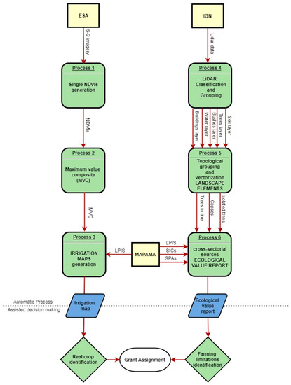
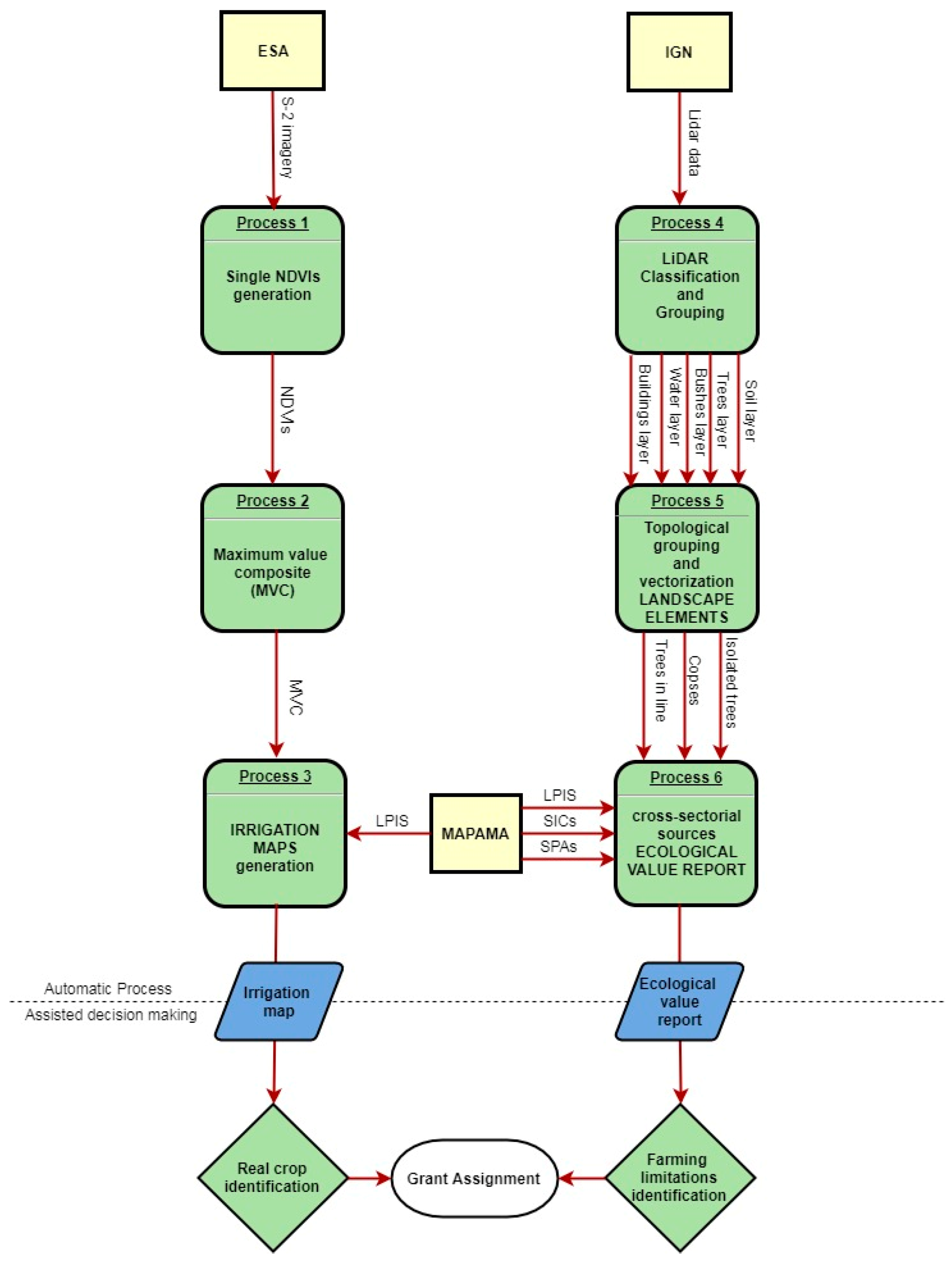
Figure 1 provides an overview of the proposed data processing workflow, illustrating the evolution of the different datasets, their transformations and their integration to generate the final products that can be used for the identification of features on agricultural parcels to be used for CAP funds assignments.

Figure 1. Data processing workflow: from original datasets to agricultural parameters’ definition. Squares represent sources of information. Rounded rectangles represent automatic processes. Parallelograms show outputs. Rhombuses represent decisions. The white shape tells where the flowchart ends. LPIS, Land Parcel Identification System; SPA, Special Protection Area for Birds; MAPAMA, Spanish Environment and Agriculture Ministry; IGN, Spanish National Geographic Institute; SIC, Site of Community Interest.

For the purpose of this paper, we consider three different sources that provide freely-available data needed to generate new products to be used in CAP grant assignment. The European Space Agency (ESA) makes available Sentinel-2 files, which are openly accessible [20] at the Sentinels Scientific Data Hub [21] as raster images (JPEG2000). For LiDAR data, we make use of the LiDAR files provided by the Spanish National Geographic Institute (IGN) [22]. Furthermore, we make use of contextualized data that are needed specifically for the task of CAP funds assignments. These include agricultural and environment datasets such as the Land Parcel Identification System (LPIS), Sites of Community Interest (SCIs) or Special Protection Areas (SPAs) for Birds (both being the last constituent parts of NATURA 2000 Network) provided by the Spanish Environment and Agriculture Ministry (MAPAMA) [23]. Based on these datasets, several automatic processes have been developed in order to obtain the final outputs.

Our irrigation type classification algorithm is applied on Sentinel-2 tiles. The tiles are the minimum indivisible partition of a Sentinel-2 product; they are 100 km² orthophotos in UTM/WGS84 projection. We begin generating a Normalized Difference Vegetation Index (NDVI) [24] from each available tile (Process 1). Then, the different layers obtained are combined in a monthly Maximum Value Composite (MVC) (Process 2). Following the MVC creation, it is necessary to extract index patterns related to the behavior of specific crops. These data are used to build a decision rule model, which estimates irrigation patterns in LPIS parcels (Process 3). The final irrigation map will show in which season each parcel is irrigated.

On the other hand, the LiDAR algorithm classifies and groups the point cloud by height, obtaining five different rasters (images), which define the main vegetation categories and other land covers (Process 4). Those auxiliary rasters are combined into one single raster, which is topologically processed and vectorized to obtain connected areas as polygons or points (Process 5), which have a direct correspondence with the landscape elements (isolated trees, copses and hedgerows).

Finally, the overlap and intersection of them with cadastral parcels (LPIS) and NATURA 2000 protected sites (SCIs and SPAs) help to generate an accurate ecological value report (Process 6). This ecological value is a score per parcel related to its protected area (under NATURA 2000 Directive), its area occupied by landscape elements and the overlap between both surfaces.

The evaluation of the landscape elements together with the presence/absence of NATURA 2000 protected sites in a specific parcel allows an estimation of the accessibility of CAP payments to farmers, taking into account that those areas become unproductive, and regarding to the cross-compliance principles.

The irrigation maps and the ecological value report will be used for supporting photo interpretation of the agricultural parcels for which CAP aid is requested. The former will help to identify the actual crop within a parcel, while the latter will assist with detecting the presence/absence of areas that have to be mandatorily protected. A physical inspection in the field should be made of all agricultural parcels for which photo interpretation does not make it possible to verify the accuracy of the declaration to the satisfaction of the competent authority.

3. Materials and Methods

3.1. Processing Sentinel-2 Data

3.1.1. Data Processing Overview

The aim of Sentinel-2 data processing is to generate maps of irrigation patterns in crops, with a 10-m pixel size. In order to identify those irrigation patterns, the evolution of the NDVI [25] was used to build a classification algorithm. This model has to be adapted for the predominant crops and agro climatic characteristics of each area.

To begin with, it is necessary to gather all of the available images, with low cloud coverage, all over the span of the agronomic cycles. Once the images are collected, an NDVI is generated for each of them. NDVI is calculated with bands of the red and the Near Infrared (NIR) spectral region, with the following formula [24]:

$$\mathrm{NDVI}=\left(\mathrm{NIR}-\mathrm{Red}\right)÷\left(\mathrm{NIR}+\mathrm{Red}\right)$$

The Sentinel-2 spectral bands used for the NDVI calculation were Bands 4 (red region) and 8A (near infrared region). The latter has a 20-m pixel size, so it was resampled at 10 m by nearest neighbor interpolation using ERDAS Imagine 2015 software (Hexagon Geospatial). Sentinel-2 provides two spectral bands in the NIR spectral domain, Bands 8 and 8A, the latter selected for its similarity with the Landsat 8 NIR band [26]. This is particularly useful to fill an eventual gap in Sentinel-2A series. No atmospheric correction was applied to the Sentinel-2 bands.

Prior to the application of the algorithm, the NDVI layers generated are combined into an MVC. The pixel values of the MVC layer correspond to the maximum NDVI value per month in order to minimize the cloud and shade coverage.

Once the MVC is created, it is inserted into a classification algorithm as an input feature. This algorithm for irrigation pattern classification is a decision tree algorithm based on the different spectral responses of crops grouped according to their phenological evolution. The decision rules of the algorithm were designed to model the entire time series and can be adapted to the characteristics of the area when spectral signatures are available.

Several studies show that incorporating the variability or range of the NDVI values across seasons delineates irrigated from non-irrigated areas more accurately than maximum NDVI data alone can do [27]. The algorithm classifies the MVC taking into account when the NDVI reaches its maximum values and how high are those values.

According to the date of the maximum value, the crops are classified into “spring”, “summer” and “spring-summer” crops. With regard to the maximum NDVI value, the crops are classified into low and high activity crops.

Following this classification, it is necessary to apply a mask to split herbaceous and woody crops. This can be done by using LPIS data. In LPIS, the different parcels are classified into numerous uses according to the species planted, structure of the crop, etc. These uses are not suitable for our classification; therefore, we generated an LPIS mask by grouping together the uses as presented in Table 1.

Table 1. Classification of land parcel identification system uses.

Groups Created	LPIS Uses *
Herbaceous crops	Arable land TA
	Orchards TH
	Greenhouses IV
Woody crops	Vineyard VI, VO and VF
	Olive trees OV, OF and OC
	Fruit trees FY and FF
	Nuts, FS, FV and FL
	Citrus CI, CV, CF and CS
Grazing land	Pasture lands PS
	Grasslands with shrubs PR
	Grassland with trees PA
Forests	Forests FO
Other uses (Non Productive)	Water AG Buildings ED Non productive IM Roads CA Urban areas ZU Censored areas ZV Not included areas ZC

* All acronyms are in Spanish. For example, TA stands for “Terreno Arable”, They can be consulted in [28].

Studies of agricultural lands have shown that NDVI is a good indicator of irrigation in Spain [29]. A high NDVI value is related to the availability of water; thus, in months with low precipitation, a high activity is only possible by irrigation. However, when the precipitation is higher, the only method to confirm that there is irrigation is using ancillary data. The data chosen for this purpose is the irrigation ratio, which can be found in LPIS. This ratio indicates the percentage of irrigated surface in a given parcel.

3.1.2. Evaluation

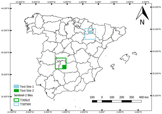
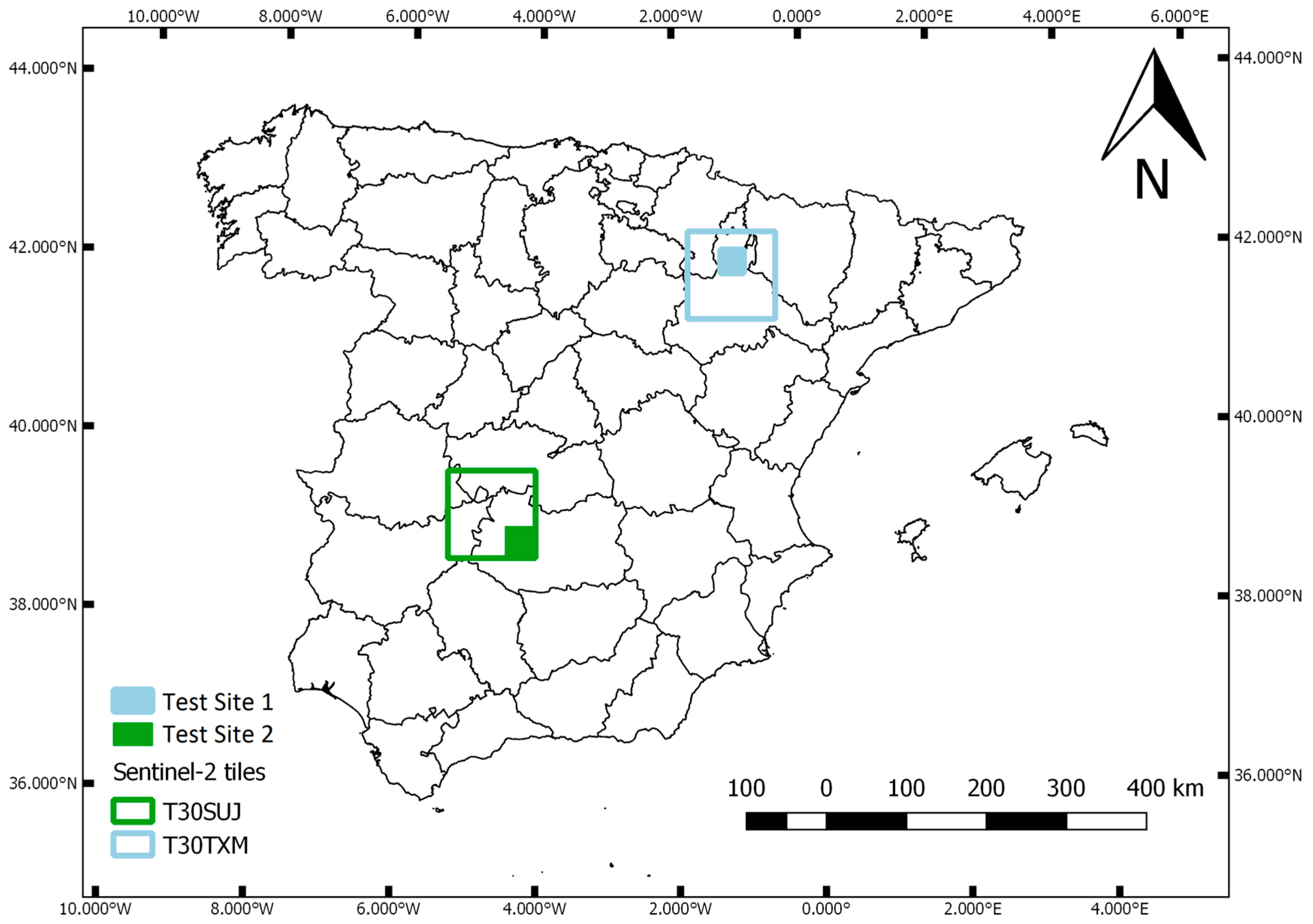
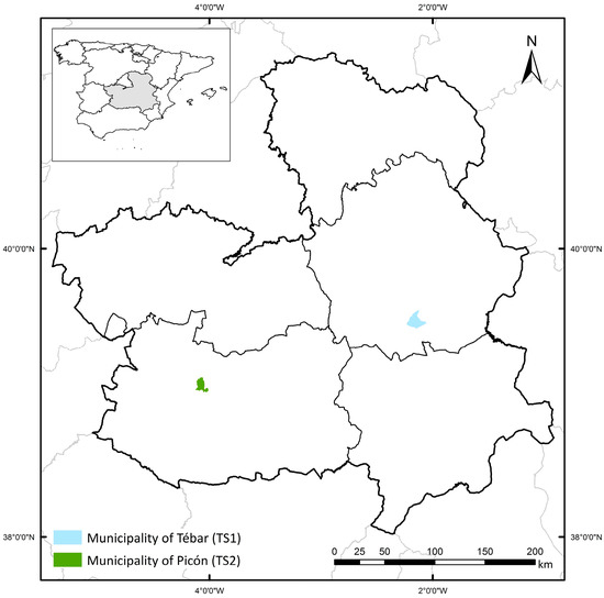
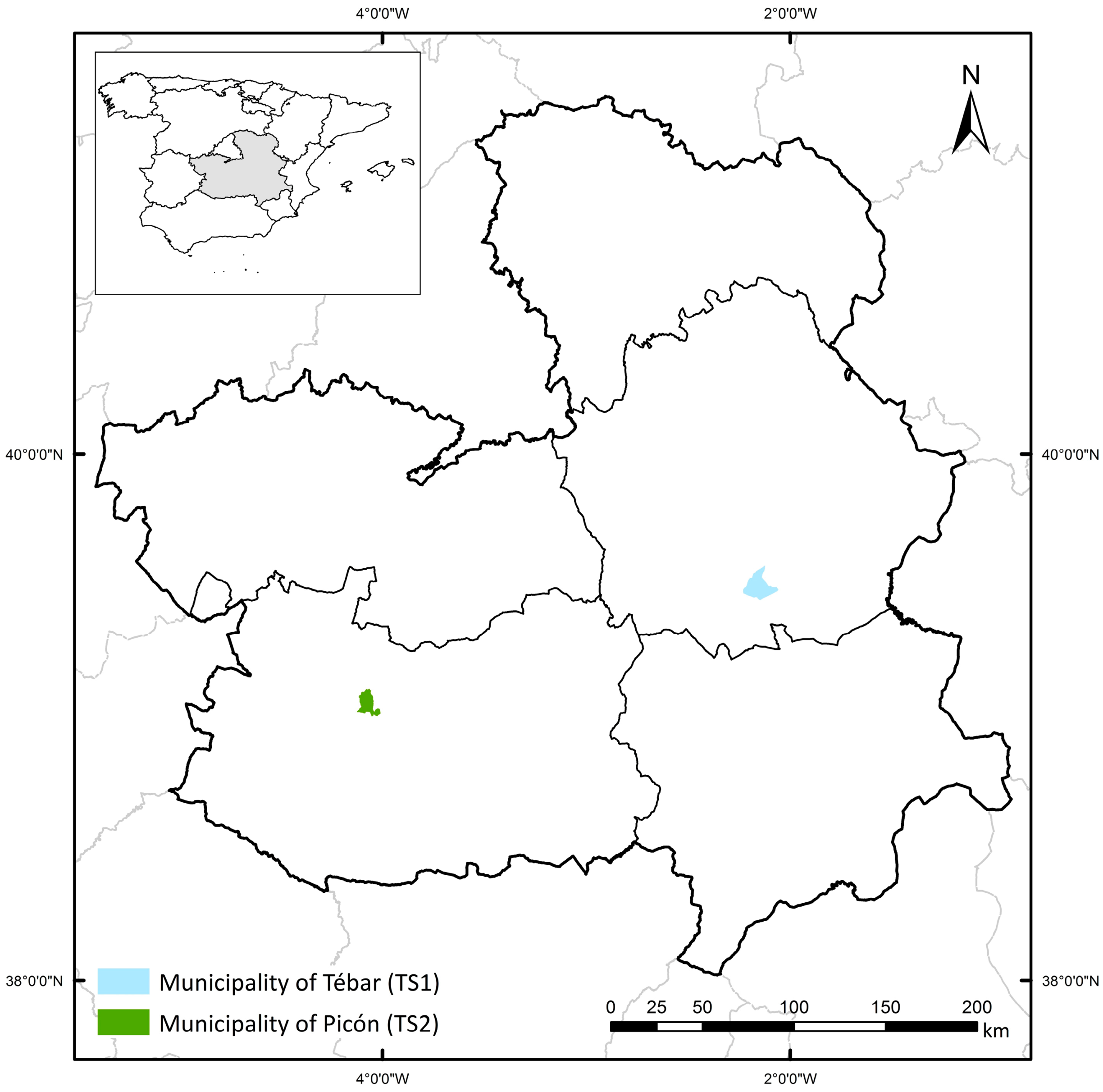
The algorithm outlined above was evaluated in two test sites, as depicted in Figure 2. Test Site 1 (TS1) is located in the northern half of the Iberian Peninsula, in the province of Zaragoza. It is close to the Ebro, one of the most important rivers of Spain. The audited area covers 40 × 40 km², and it is mainly covered by irrigated crops. The whole surveyed area is within the Sentinel-2 tile T30TXM. Test Site 2 (TS2) is in the province of Ciudad Real, in the southern half of the Iberian Peninsula. It covers an area of about 50 × 50 km² within the Sentinel-2 tile T30SUJ. This zone has a small surface of regularly-irrigated crops.

Figure 2. Pilot areas distribution.

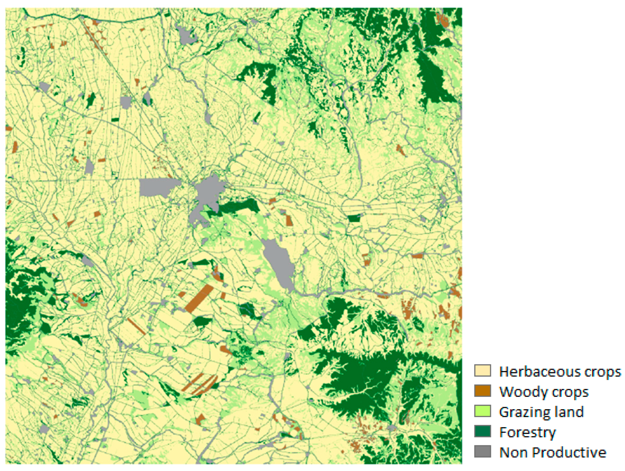
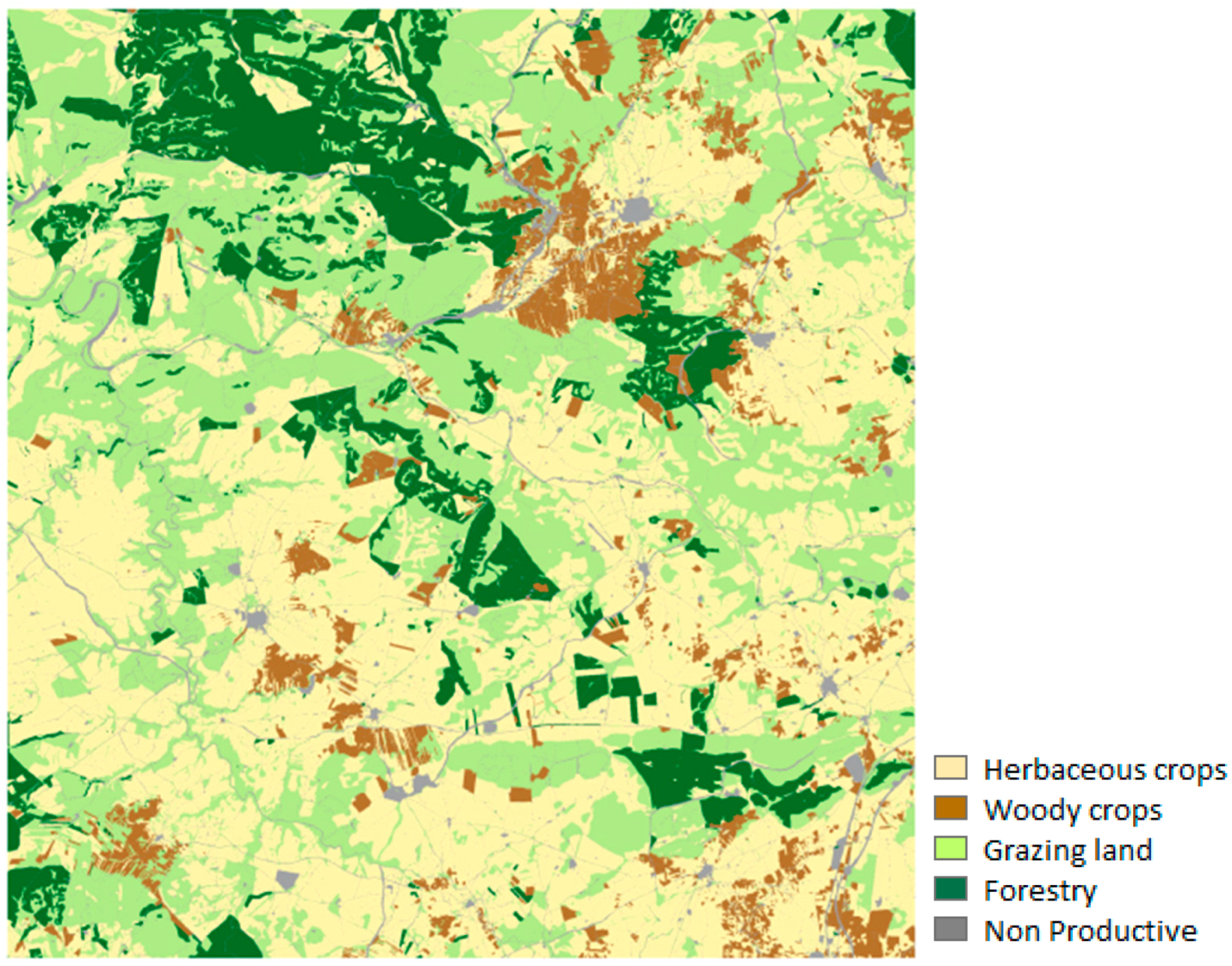
These areas were chosen because they were audited by the Spanish public administration in 2016; therefore, it is possible to compare the real and automatic generated data. Another advantage of using these test sites is that LPIS data for both areas are freely available. Due to the fact that woody crops are scarce in both areas (see Figure 3 and Figure 4), only data about herbaceous crops were surveyed. Thus, in the following, we only classify this type of crop.

Figure 3. Land use classification in TS1 obtained from LPIS.

Figure 4. Land use classification in TS2 obtained from LPIS.

The dates in which Sentinel-2A took images in the test sites fitting our selection criteria are shown in Table 2.

Table 2. Sensing date of the imagery used in the test sites. TS1, Test Site 1.

Month	TS1 (T30TXM Tile)	TS2 (T30SUJ Tile)
December	3 December 2015	29 November 2015 *, 6 December 2015, 19 December 2015
January	5 January 2016, 12 January 2016	There are not images with low cloud coverage in this month
February	4 February 2016	4 February 2016, 17 February 2016
March	12 March 2016, 22 March 2016	25 March 2016
April	1 April 2016	7 April 2016, 14 April 2016, 24 April 2016
May	4 May 2016, 21 May 2016	27 May 2016
June	23 May 2016	13 June 2016, 23 June 2016
July	3 July 2016, 30 July 2016	3 July 2016, 13 July2016, 16 July 2016, 23 July 2016, 26 July2016
August	2 August 2016, 12 August 2016, 22 August 2016	2 August 2016, 5 August 2016, 12 August 2016, 22 August 2016

* In December, the images have high cloud coverage, so this one was considered as a December image in order to fill the missing information.

In January, there are no available images for the TS2 area (T30SUJ). To solve this issue, the NDVI value of January was generated by interpolation of the values of December and February.

The LPIS masks generated for both test sites are shown in Figure 3 and Figure 4.

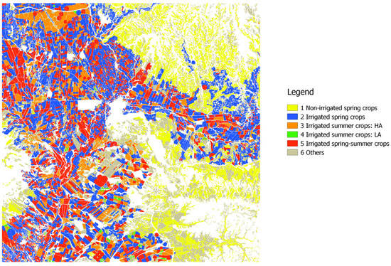
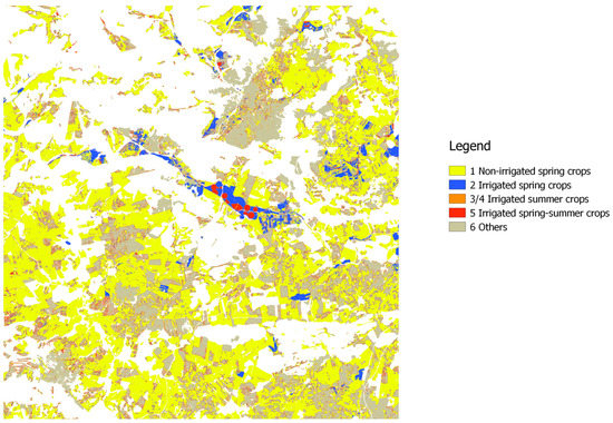
After applying the algorithm, the crops with their highest activity in April and May were classified as spring crops. High activity classes were crossed with the irrigation ratio from LPIS (irrigation ratio greater than 0) to obtain irrigated spring herbaceous crops (Class 2). Everything else is classified as non-irrigated spring herbaceous crops (Class 1).

The crops with a peak of activity in July, August or both were classified as summer herbaceous crops. Due to the fact that both test sites experienced a hot dry summer, these values are only possible by irrigation. Therefore, the LPIS irrigation ratio was not taken into account, and they all are classified only in regards to their vegetative activity. In TS1, they are divided into crops with high (Class 3) and low (Class 4) activity. In TS2, these differences do not exist.

The parcels classified as spring-summer crops have high activity from April–August. The only explanation is that they are irrigated during all of those months; thus, they are classified as irrigated spring-summer herbaceous crops (Class 5). Other crops were grouped into Class 6.

3.2. Processing LiDAR Data

3.2.1. Data Processing Overview

The landscape elements in Spain are regulated by the Royal Decree 1078/2014 [30], which establishes the cross-compliance principles and the funds assignments regarding environmentally- friendly land management requirements. That decree defines the landscape elements as hedges, copses, isolated trees, hedgerows, trees in group, etc., and each year, farmers could get CAP grant assignments to maintain these trees layouts. LiDAR data processing is a powerful tool to identify these elements [31] and contributes to an enhanced assessment of suitability for agricultural grant requests.

The developed LiDAR data-processing algorithm consists of a set of rules that enable automatic identification of landscape elements formed by copses, isolated trees and hedgerows. The analysis was focused on arable lands and woody crop areas considering the following free available datasets: LiDAR files in .las format [32] provided by the Spanish National Geographic Institute; and the Land Parcel Identification System shapefile [33] provided by the Spanish Environment and Agriculture Ministry.

On the other hand, the orthophoto published by the Castilla La Mancha [32] region is involved in the final evaluation phase just for supporting purposes, and it is not processed by the LiDAR algorithm.

3.2.2. Point Cloud Classification

In the first stage, the .las files were processed by classifying the point cloud by height and creating different groups, which have a direct correspondence with the representative vegetation classes in Spain (Table 3). The relative height values for each point were obtained via subtraction from the underlying digital terrain model. After that, a new raster layer was created for each vegetation group in Table 3. The chosen pixel size for these layers was 5 m.

Table 3. Representative classes of LiDAR vegetation in Spain.

Vegetation Class	Vegetation Group
Soil	Soil and penetrable vegetation
Vegetation with height 0 cm–40 cm	Soil and penetrable vegetation
Vegetation with height 40 cm–60 cm	Soil and penetrable vegetation
Vegetation with height 60 cm–80 cm	Bushes
Vegetation with height 80 cm–1 m	Bushes
Vegetation with height 1 m–1.5 m	Bushes
Vegetation with height 1.5 m–2 m	Bushes
Vegetation with height 2 m–3 m	Trees
Vegetation with height 3 m–5 m	Trees
Vegetation with height 5 m–10 m	Trees
Vegetation with height >10 m	Trees
Buildings	-
Water	-

From these five layers, it is possible to generate a single raster with a 5-m pixel size adding different attributes per pixel such as the percentage of soil points, bushes, trees, buildings and water. Finally, these attributes are used to assign the final vegetation class for each pixel in accordance with the predominant category.

Once the final raster is obtained, the next steps consist of the application of different topological rules and spatial analysis in accordance with the parameters defined in the Spanish Law regarding the identification of isolated trees, copses and hedgerows.

3.2.3. Isolated Trees and Copses

The proposal methodology follows a set of rules in order to identify isolated trees and copses:

• Isolated trees must be areas between 2 and 12 pixels, which imply a surface of 50–300 m².
• Copses must be larger areas with a surface between 12 and 120 pixels, around 300–3000 m².
• The height of pixels classified as trees must be greater than 3 m or higher than 2 m when their surfaces have more than 20% of points with a height over 3 m.
• Pixels may contact with bush classes; however, when the perimeter of this contact is greater than 25% and contains points over 3 m of altitude, the class will be considered as an isolated tree.
• The distance between 2 pixels or a group of pixels must be at least 5 m.

3.2.4. Hedgerows

The initial identification rules considered were similar to the guidelines explained above. However, after a series of tests, the conclusion was that further analysis is required to properly identify these elements. The methodology must include shape index analysis, considering the surface and the perimeters of these trees’ areas.

The identification of hedgerows is a complex process. For this reason, the first step is selecting surfaces larger than 3000 m² since smaller areas will belong to isolated trees or copses regardless of their shape. Regarding these parameters, hedgerows must have the following characteristics:

• Surface over 3000 m².
• Their surface must have at least 20% of points with a height over 3 m.
• Their perimeter of contact with the bushes class must be less than 25%.
• Their surface divided by their perimeter must be less than 5.
• The square root of the previous index must be less than 0.1.

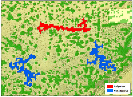
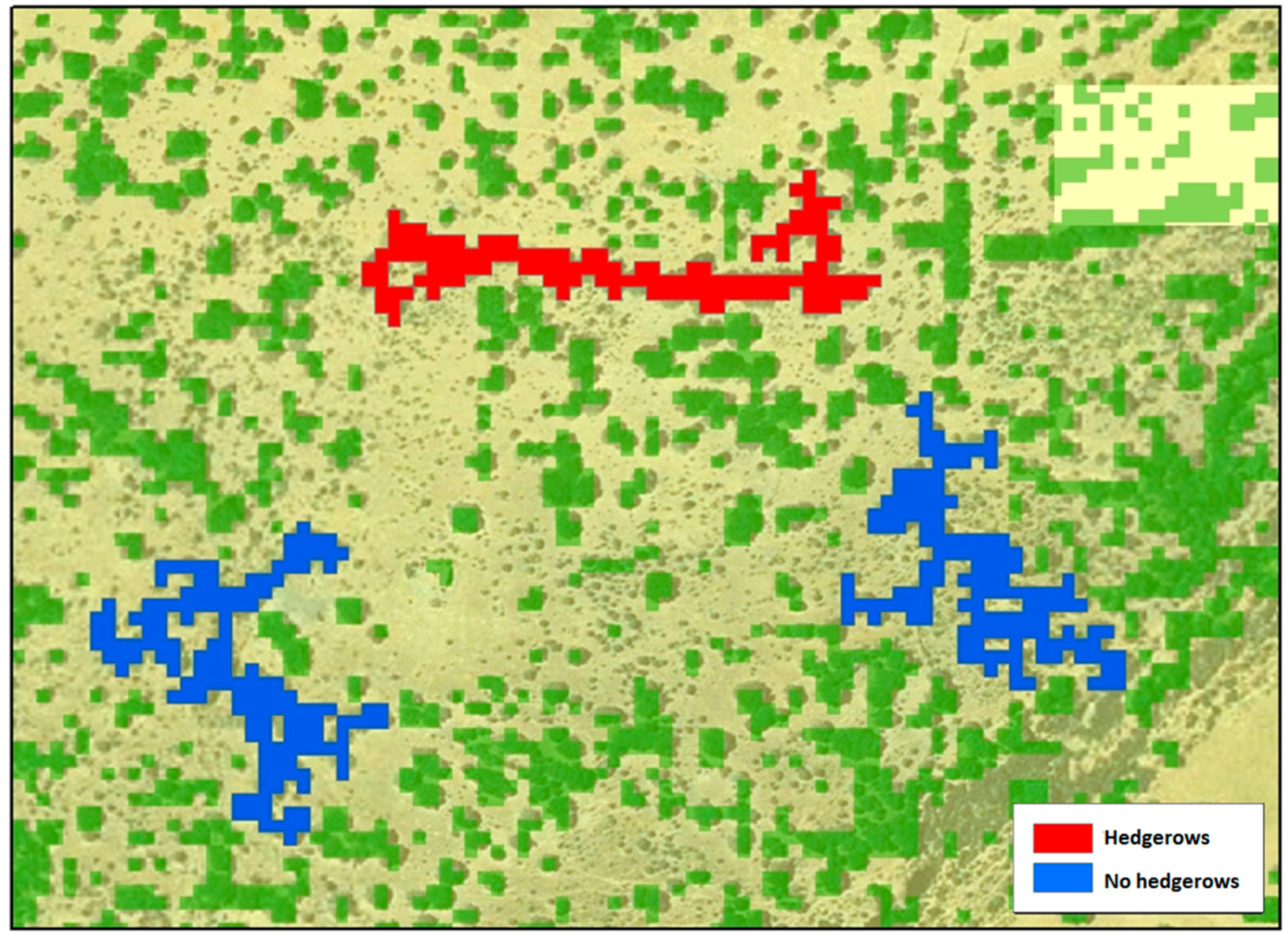
Figure 5 shows different results of this process.

Figure 5. Result of hedgerows identification. Areas represented in red are identified as hedgerows, while blue areas are discarded.

3.2.5. Evaluation

In order to check whether the generated data are reliable or not, two cadastral polygons situated in Castilla La Mancha (center of Spain) were chosen, as can be seen in Figure 6. These sites were selected because they have a significant amount of different landscape elements. The first test site is a cadastral polygon situated in the municipality of Tébar in the province of Cuenca. This pilot area has a surface of around 7 km², and its predominant land covers are arable lands and shrub grass plus some small areas with vineyards and fruit trees. This test site was previously selected to identify the landscape elements by photointerpretation, finding a significant number of isolated trees to compare the results between the automatic process and the manual operations.

Figure 6. Selected areas for LiDAR processing evaluation.

The second test site is a cadastral polygon situated in the municipality of Picón in the province of Ciudad Real. It has the same characteristics as the previous one regarding its land covers and surface; nevertheless, in this test area, the number of photo interpreted areas as copses is significant enough to carry out relevant studies.

3.2.6. Ecological Assessment

The results obtained in the evaluation of LiDAR processing make it possible to perform an ecological assessment of the parcels. The ecological assessment represents an estimation of the area inside of a parcel that has to be mandatorily protected and, therefore, become unproductive under cross-compliance principles and NATURA 2000 Directive. For that purpose, once the mentioned landscape elements are refined and vectorized, they can be evaluated according to other ecologic parameters such as:

• Crop diversification;
• Type, density and surface of ecological focus areas;
• Proximity or overlapping to natural parks and protected sites;
• Proximity or overlapping to Sites of Community Interest (SICs);
• Proximity of overlapping to Special Protection Areas (SPAs) for birds.

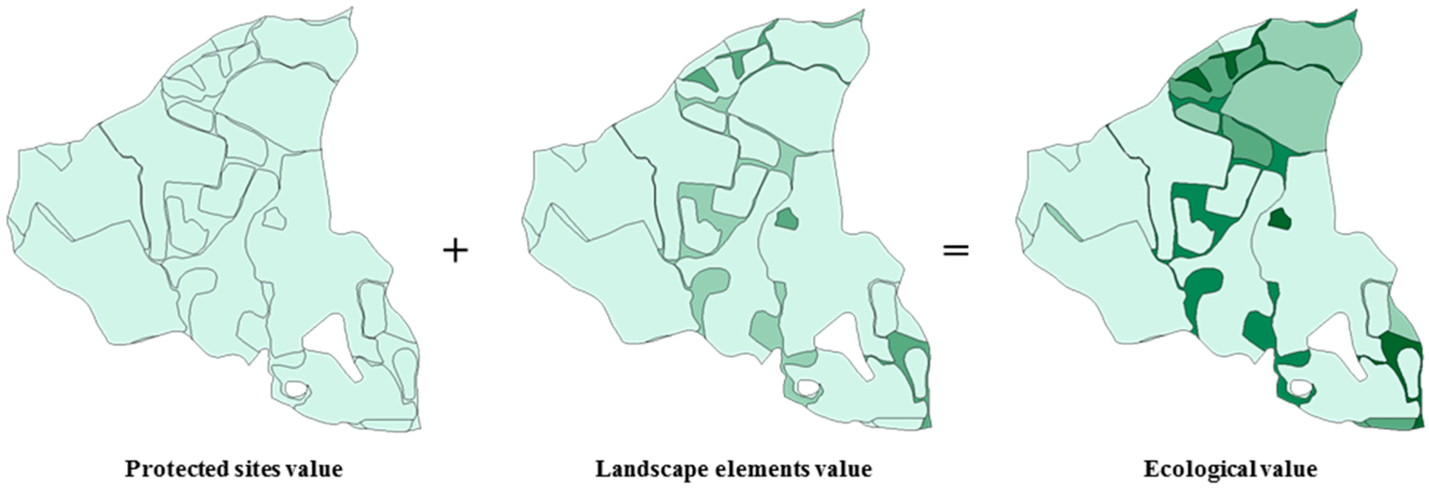
In the LiDAR methodology, protected sites of the NATURA 2000 Network, copses, isolated trees and cadastral parcels were used to design an accurate ecological value report for Spanish crop areas, obtaining the layers protected sites value, landscape elements value and ecological value. They are obtained from the queries in Table 4.

Table 4. Queries for generating the ecological value report.

	Meaning	Score
Query 1	Surface of Sites of Community Interest/subplot area.	0–1
Query 2	Surface of Special Protection Areas for Birds/subplot area.	0–1
Query 3	Number of isolated trees/subplot area.	0–1
Query 4	Surface of copses area/subplot area.	0–1
Protected sites value	This vector layer is the result of the sum of Query 1 and Query 2	0–2
Landscape elements value	This vector layer is the result of the sum of Query 3 and Query 4.	0–2
Ecological value	This vector layer is the result of the sum of protected sites value plus landscape elements value.	0–4

Finally, the proposed LiDAR algorithm allows us to obtain more detailed information per cadastral parcel (land property comes from LPIS) because the landscape value helps to identify which subplot (land use comes from LPIS) has more value per parcel, from the environmental point of view.

On the other hand, from the point of view of CAP payment assignments, the final score coming from the ecological value report helps to make estimations about the economic aids for farmers, considering the areas that became unproductive and the subject of strict protection. In this way, the public administration encourages farmers to maintain these agricultural ecosystems via an economic aid regulated through the CAP requirements.

4. Results

4.1. Irrigation Maps

Sentinel-2 classification for TS1 and TS2 can be observed in Figure 7 and Figure 8.

Figure 7. TS1 Irrigation map.

Figure 8. TS2 Irrigation map.

To validate our results, we used data collected during a field visit in 2016. The accuracies obtained are presented in Table 5.

Table 5. User’s and overall accuracy of the Sentinel-2 data processing algorithm. Reference data for the ratio of correctly-classified pixels were acquired during field surveys at the test sites.

Class	TS1	TS2
Spring Herb	87.94%	95.15%
Summer Herb	88.79%	NA
Spring-Summer Herb	87.24%	NA
Overall accuracy	85.64%	95.55%

The field data in TS2 do not include summer crops since the field visit took place in spring. Moreover, there is a small number of lands for forage (less than 3 ha, which would be included in the group of crops with activity during spring and summer).

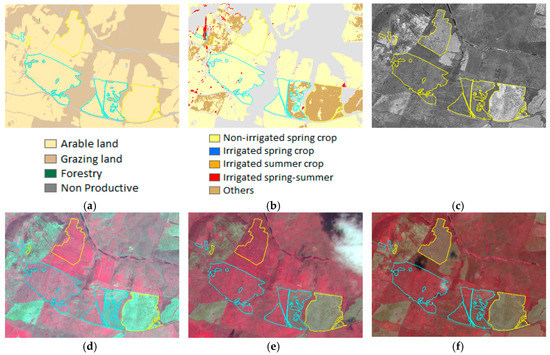
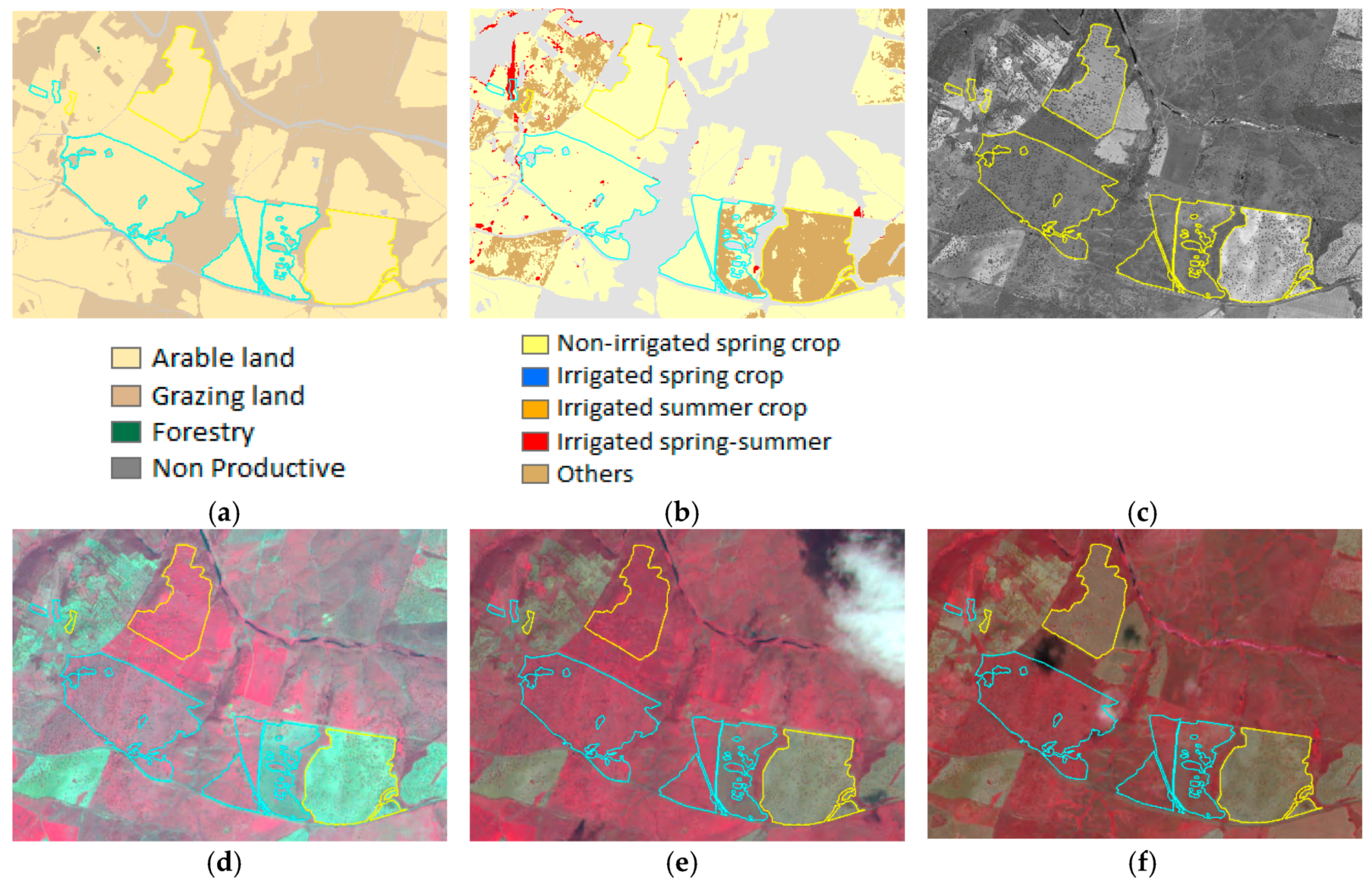
The main misclassification was found in grassland areas in TS2, which are inside of the LPIS arable lands mask. They were assigned to non-irrigated spring crops. The algorithm was not created for dealing with grasslands, but with agriculture crops. Theoretically, grasslands should be classified as “others”. However, both ‘grasslands’ and ‘others’ include a wide range of typologies; therefore, it is not a surprise that they were assigned to non-irrigated spring crops. Some grassland areas have activity in spring, but not in summer, and they are not irrigated. The solution to this classification problem is using ancillary data to have a correct delimitation of the non-agricultural classes.

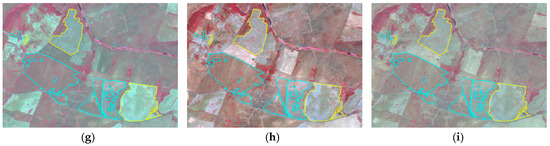
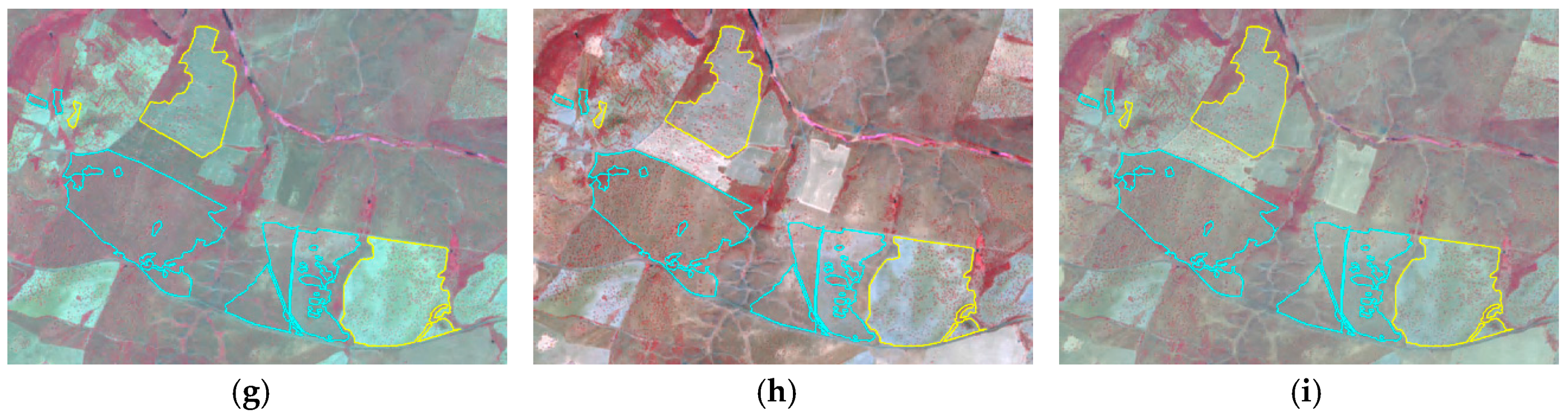
If we include grasslands within non-irrigated spring crops, the overall accuracy of the classification is about 96%. If we consider grassland samples as a misclassification, the overall accuracy drops to 73%. In Figure 9, we include examples of grassland areas that come from the validation sample (cyan polygons), which in the classification have been assigned either to “non-irrigated spring herbaceous crops with low activity” or to “other crops”.

Figure 9. TS2 validation images. Cyan polygons are grassland areas that were classified as “non-irrigated spring herbaceous crops with low activity” or as “other crops”. Yellow polygons represent agricultural parcels. (a) LPIS data; (b) Arable land classification; (c) VHR image of spring 2016: Polygons in yellow to enhance visualization; (d) Sentinel-2 infrared composite. Date: 25 March 2016; (e) Sentinel-2 infrared composite Date: 14 April 2016; (f) Sentinel-2 infrared composite Date: 27 May 2016; (g) Sentinel-2 infrared composite Date: 13 June 2016; (h) Sentinel-2 infrared composite Date: 26 July 2016; (i) Sentinel-2 infrared composite Date: 12 August 2016.

4.2. Landscape Elements

In the first test site, 248 isolated trees were identified by human operators. Over this total amount, 224 trees were successfully detected through LiDAR processing, which implies an overall accuracy in the classification of isolated trees of about 90.32%. Errors of omission (unidentified isolated trees) are more frequent than errors of commission (identified isolated trees that are not), as can be seen in Table 6.

Table 6. Results of the evaluation in the classification of isolated trees.

Total Isolated Trees Identified	Errors of Omission		Errors of Commission
	Num. of Errors	% Error	Num. of Errors	% Error
248	20	8.0645	4	1.613

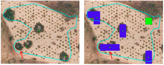
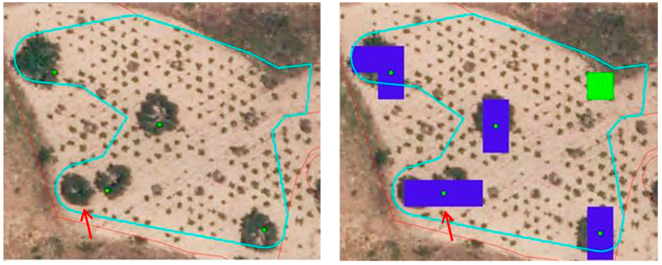
Most of errors of omission were over small trees with canopies smaller than 4 m and, in other cases (Figure 10), due to pixels classified, as isolated trees include two trees, and only one of them was identified. Pixels in blue represent woody areas, while green pixels are over scrub coverings. The red arrow points to a missing isolated tree in the classification as a consequence of two pixels that were considered only as one isolated tree.

Figure 10. Errors of omission in the classification of isolated trees.

Further, the errors of commission were produced over built elements. In the test area, these elements are wind generators, which in some cases were classified as building and in other cases as isolated trees.

In TS2, 30 fragments were identified as copses with an average area around 717 m², while LiDAR processing detected 90 features, which cover all photo interpreted areas with a similar average area. In this instance, the overall accuracy in the classification of copses is about 67.48%, and the most common errors were produced due to commission; in other words, there are more pixels incorrectly classified as copses.

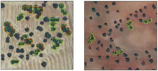
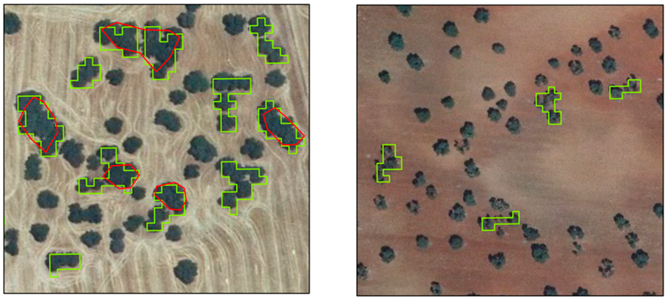
However, as shown in Figure 11, this is due to the square borders of raster data processing, and in other situations, they were mistakes made by the human operators, which demonstrate the subjectivity of the manual process. Photo interpreted copses are represented under red borders and copses coming from the automatic classification are outlined in green. On the left, square and regular edges can be observed below the manual digitalization. On the right, there are some examples of copses identified by automatic classification that were not classified by human operators.

Figure 11. Errors of commission in the classification of copses.

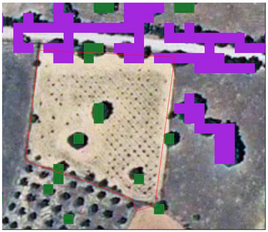
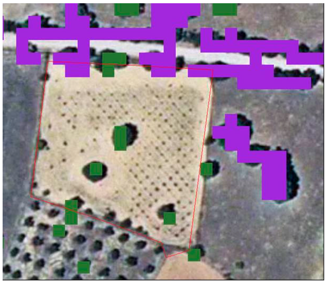
A common point between the automatic classification of isolated trees and copses is that their identification over woody crop areas is not accurate due to the difficulty to differentiate the woody crops (with height between 2 and 3 m) and dispersed trees considered as landscape elements. However, inside woody crop areas with a low density and a smaller size of their canopy, the identification obtains a higher precision, as shown in Figure 12.

Figure 12. Detection of copses (in purple) and isolated trees (in green) around woody crop areas.

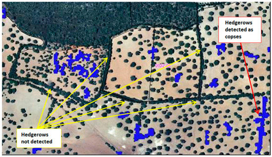
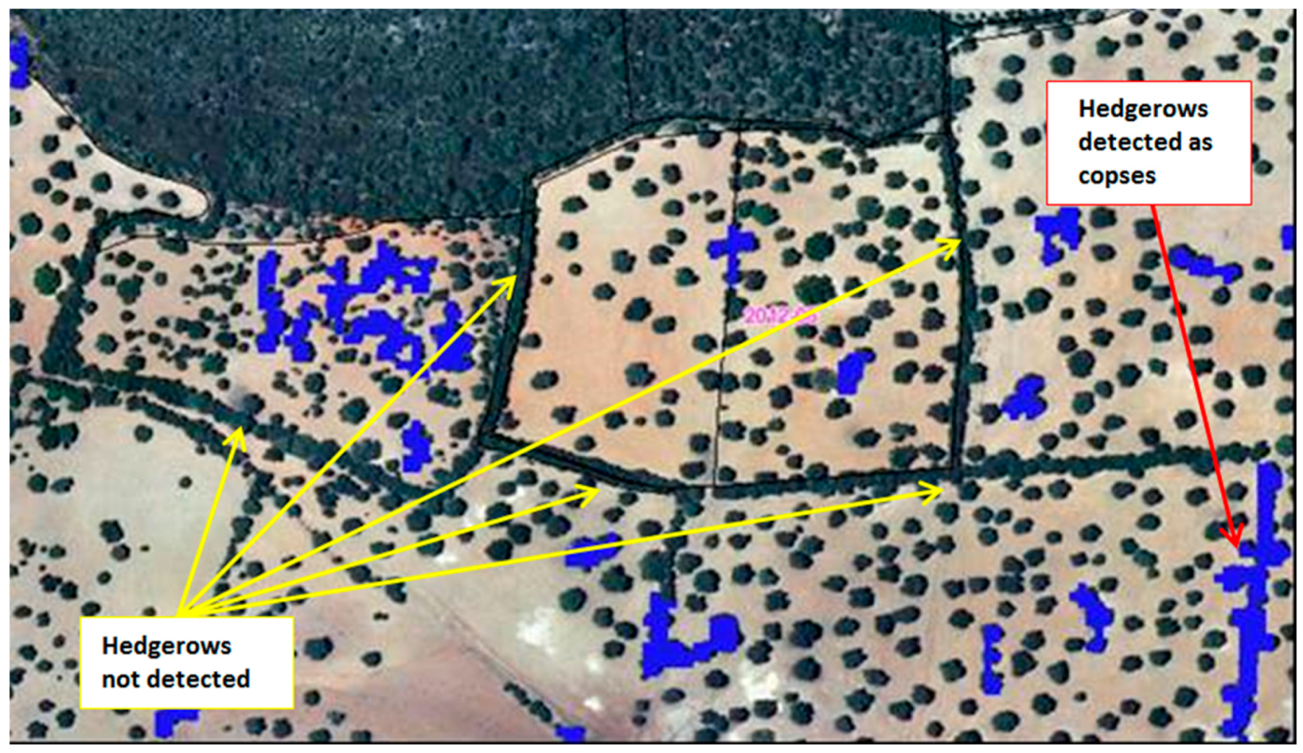
On the other side, in the evaluation of the automatic classification of hedgerows, only a few areas were detected, obtaining a percentage of errors due to omission over 75%. These errors are the consequence of two factors that can be observed in Figure 13:

Figure 13. Limitations in hedgerows detection.

• Some hedgerows areas were identified as copses because their size was smaller than 3000 m²;
• Other areas were not detected because they were connected with bigger trees surfaces.

Apart from these limitations, the high percentage of the identification of isolated trees and copses allows a direct upload to the database through the transformation of the original raster layers in vector files. For that purpose, pixels classified as isolated trees were vectorized through their centroid point, and pixels identified as copses were vectorized as polygon features.

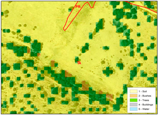
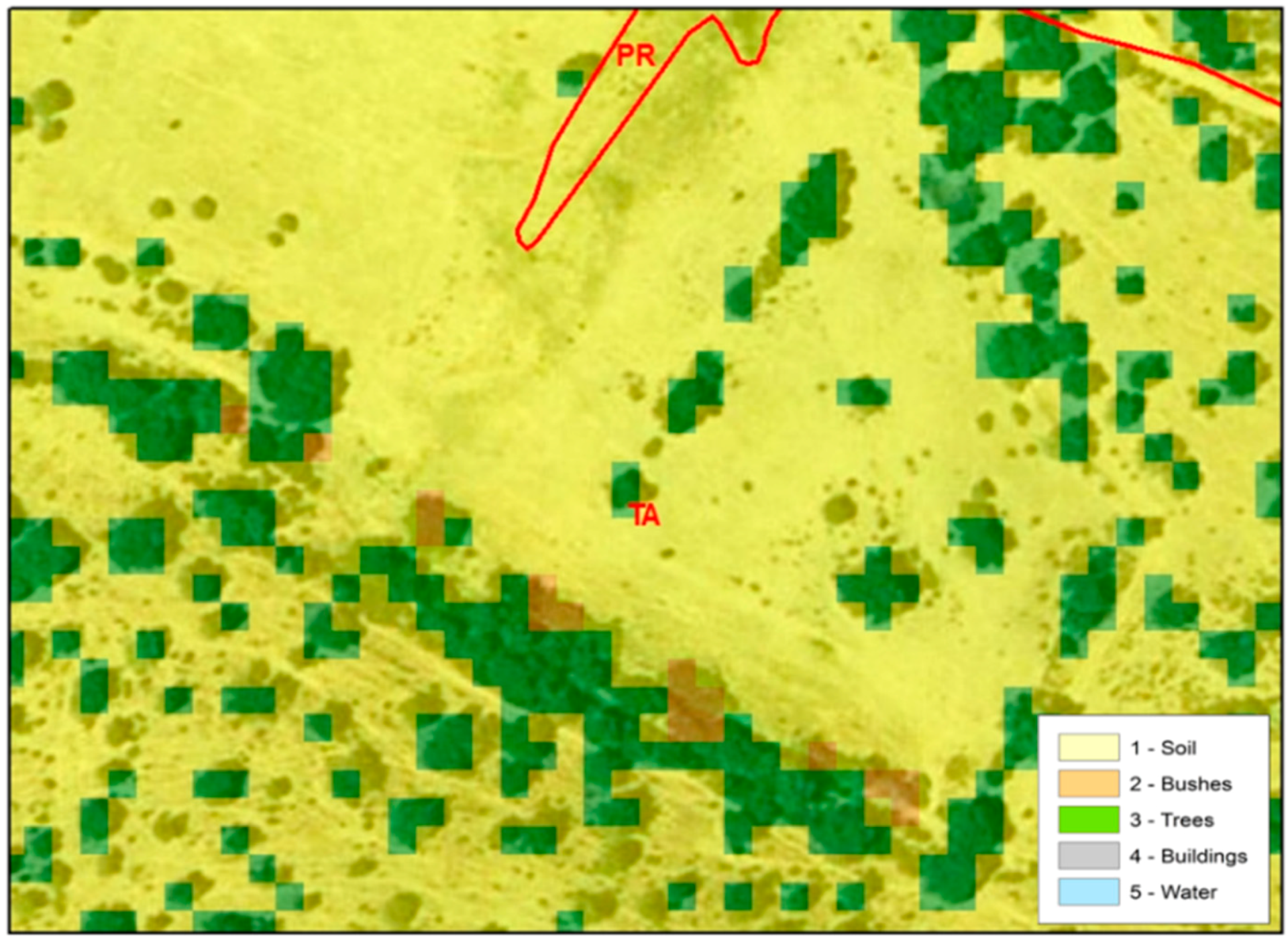
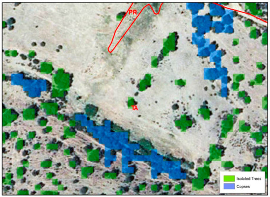
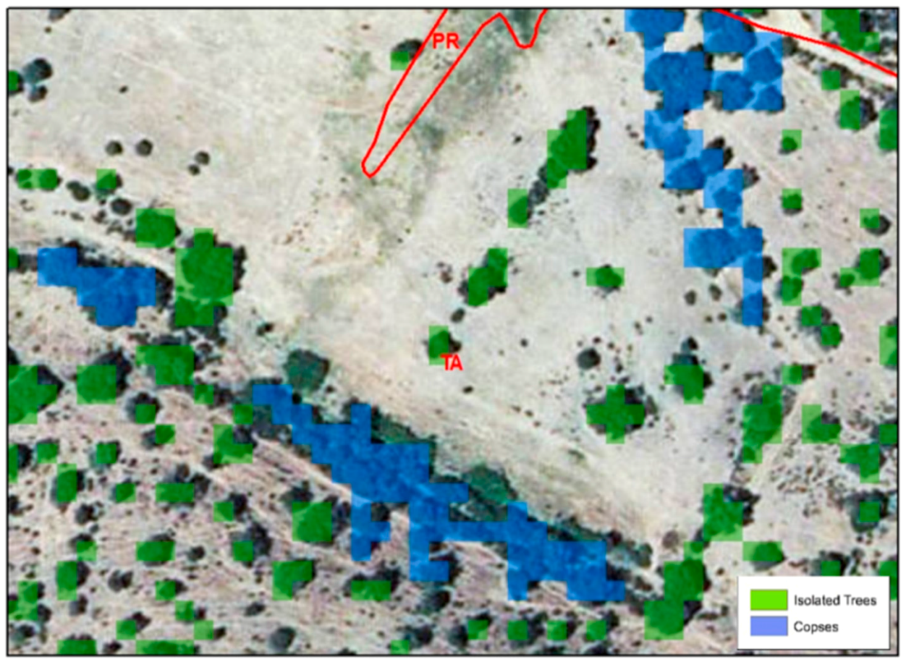
Figure 14 and Figure 15 show examples of the pixel classification and the identification of isolated trees and copses.

Figure 14. Raster with the final class for each pixel: soil (yellow), bushes (orange) and tree groups (green).

Figure 15. Identification of isolated trees and copses. Isolated trees are represented in green color, and copses are in blue areas.

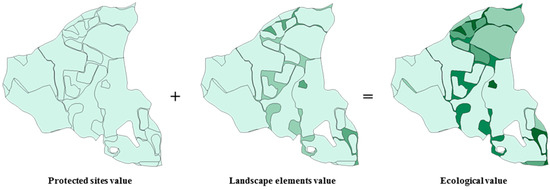
The landscape elements layers can be combined with protected sites data in order to obtain an ecological value report as shown in Figure 16.

Figure 16. Parcel sample showing the ecological value report; the result of the added values from protected sites and landscape elements.

5. Related Works

The performance characteristics of Sentinel-2 for crop and forest classification were first analyzed by Immitzer et al. [13]. A species classification was assayed by using 10 Sentinel-2 spectral bands for a single date in a random forest classification. The main disadvantage of this method for our purpose is that multi-temporal analysis has greater potential to define irrigated areas [34]. A random forest classification method could be used for irrigation maps as long as data from different dates is included in the random forest classification.

In our approach, we use NDVI time series for its usability in surrogating vegetation activity [25,35]. The NDVI properties help mitigate a large part of the variations that result from the overall remote sensing system (radiometric, spectral, calibration, noise, viewing geometry and changing atmospheric conditions) [31]. A large body of literature has researched the usefulness of NDVI for irrigation mapping [36]; however, previous studies have not dealt with using Sentinel-2 for this purpose.

There are many experiences with vegetation mapping through LiDAR data [15,19,31,37], but none of them were applied for the automatic identification of the landscape elements as they are defined in the CAP requirements.

The special report elaborated by European Courts of Auditors “The Land Parcel Identification System: a useful tool to determine the eligibility of agricultural land—but its management could be further improved” [38] says that “one way to mitigate the risk of incorrectly registering eligible area in an LPIS and to achieve more objective results is to develop and apply automatic change-detection tools”.

Member States such as Austria and Ireland were giving consideration to a range of such tools for LPIS data interpretation; however, all of them are using satellite imagery; therefore, LiDAR technologies are currently underused. In the case of the Ecological Focus Areas (EFAs) layer, which includes information about the landscape elements, Member States have to register all permanent ecological focus areas in a layer in their LPIS by 2018. However, 26 out of 44 Member States are still beginning to make their first inventories through digitization by human operators. Other regions, such as Scotland (United Kingdom), have not yet digitized any EFAs, or others, such as North Rhine Westphalia (Germany), have not correctly determined the EFA categories and their sizes in all cases, leading to miscalculations, since the coefficients are different for certain elements, such as hedges or field copses, for example.

The Spanish use case for the automatic identification of these elements may be an opportunity to meet the requirements and commitments of the CAP regulations. Likewise, many European countries have started to make their LiDAR data openly available, which may provide an improvement of the data reliability and using innovative techniques, in order to both improve accuracy and reduce administrative costs.

A detailed comparison of methods used in related works would be a fruitful area for further research, as it would help us to establish a greater degree of accuracy on CAP grant assignment.

6. Discussion and Outlook

In this paper, we proposed a method for processing and integration of multi-sectorial data from several sources into the existing data of the Spanish CAP Payment Agency, a method that can produce better and fairer Common Agriculture Policy (CAP) funds assignments to farmers and land owners. Such a public agency has to trust data submitted by owners or managers (stakeholders) that could be incorrect or inaccurate. Therefore, an unfair grant assignment and expenditure on audits and field visits would be a direct result. However, not only this, but an inaccurate specification of the kind of crop or the surface of the Ecological Focus Areas (EFAs) turns out to be an incorrect grant assignment for farmers.

Accordingly, the use of the external, and usually underused data sources, such as the ones highlighted in Figure 1, offers a powerful and accurate tool for generating new contrast and validation data for the information used by the Spanish CAP Payment Agency.

As explained in Section 2, the irrigation patterns obtained from Sentinel-2 were successful, as they were able to identify when the crops are irrigated. The high Sentinel-2 revisit time permits the collection of dense time series without important gaps. This characteristic of Sentinel-2 along with its high resolution allowed us to identify agricultural areas with a high accuracy. In terms of directions for future work, it would be interesting to implement new indexes in the crop identification for CAP grant assignment, such as SAVI [25] or NDWI [39].

Although the method relies on ancillary data available in LPIS, this approach can be used in countries that do not have access to similar data, by splitting herbaceous and woody crops using photo interpreters. However the lack of an irrigation ratio can be a source of uncertainty in areas with high precipitation.

Though there is abundant room for further progress in determining agricultural species with Sentinel-2, more research is required to determine the effectiveness of its spectral capabilities to identify plant species.

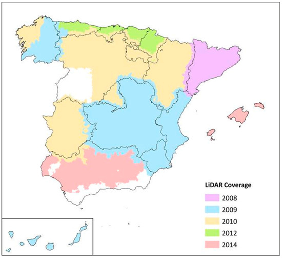
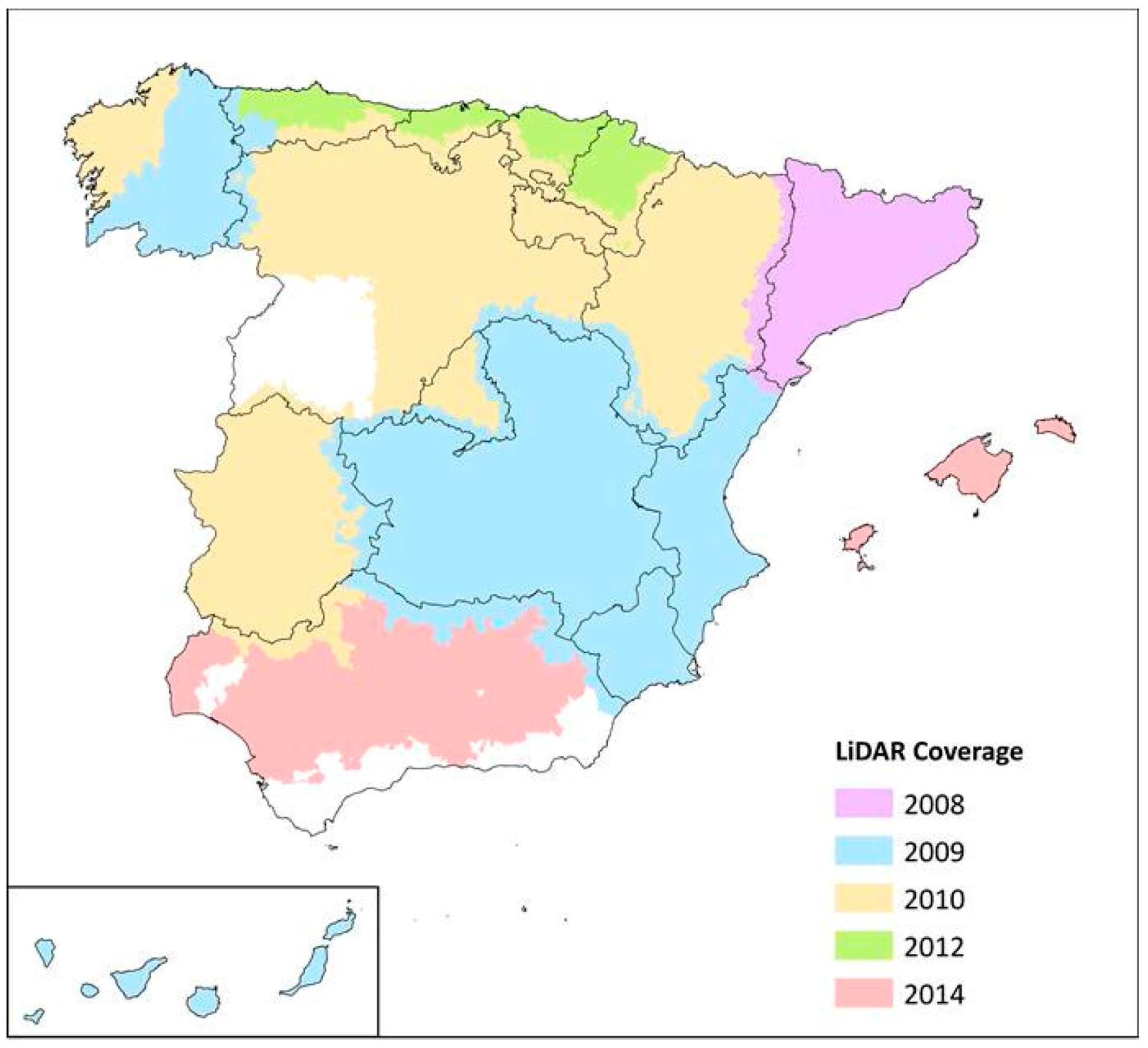
In regards to Section 3, the deployment of the LiDAR algorithm has been evaluated by the Spanish public administration as a preliminary step to the photointerpretation in the CAP control tasks. It demonstrated that the provision of the auxiliary layers coming from LiDAR facilitated the work of human operators, making it more effective and objective. Nevertheless, at this stage, the direct loading of the automatic landscape elements layer into the Spanish CAP Payment Agency production environment is not yet possible because its accuracy needs improvement. One disadvantage of LiDAR data availability is its date of coverage. As can be observed in Figure 17, in some areas, the last flights took place in 2008, while in others in 2014. For this reason, some results in the automatic detection of the landscape elements could not be completely reliable. However, currently, the LiDAR processing has the opportunity to improve its results by Sentinel-2 data, which are frequently updated, and allows checking that each feature has correspondence with vegetation areas [40]. This will make it possible to include a new process in the methodology in order to improve the accuracy in the landscape elements’ automatic detection.

Figure 17. LiDAR coverage in Spain.

On the other hand, the final outputs of LiDAR processing allow one to identify small ecosystems in agricultural environments that can be useful for ecological studies and not only to define the CAP parameters on a specific parcel. Whilst Sentinel-2 data are freely available worldwide, LiDAR data are not in most countries. Even where such data have been acquired, they may only be available at a cost to the user. Nevertheless, the overall LiDAR data processing approach presented in this paper could be reused once data become available.

Furthermore, the resulting data from the processing algorithms and case studies reported in this paper are publicly available and can be visualized via the Common Agriculture Policy Funds Assignments Service (CAPAS) viewer [41] and accessed in Linked Data form [42] via SPARQL on the DataGraft platform [43,44,45].

7. Conclusions

This study has shown that Sentinel-2 and LiDAR data can be used to generate accurate irrigation maps and ecological value reports. These datasets were generated through automatic algorithms that were analyzed in Spanish test areas yielding the following accuracies:

• The algorithm for the identification of crops’ irrigation patterns based on Sentinel-2 data yielded an overall accuracy over 85% in TS1 and over 95% in TS2;
• The algorithm for the detection of landscape elements based on LiDAR data yielded an overall accuracy between 90.32% and 67.48% depending on the element to be identified.

The use of Sentinel-2 series and LiDAR can help to detect areas that are not eligible for grant assignment, support cross-check and be used as a tool for choosing field samples. However, today, it is still necessary to use additional data (e.g., very high resolution imagery) and field visits for the right definition of agricultural features. It is expected that the massive use of Sentinel-2 imagery and LiDAR will make CAP management easier and more economically efficient.

References

- CAP at A Glance. Available online: https://ec.europa.eu/agriculture/cap-overview_en (accessed on 11 August 2017).
- Managing the Agriculture Budget Wisely. Available online: http://old.europe.bg/upload/docs/factsheet_en.pdf (accessed on 11 August 2017).
- Commission Implementing Decision of 26 April 2013 on the Clearance of the Accounts of the Paying Agencies of Member States Concerning Expenditure Financed by the European Agricultural Fund for Rural Development (EAFRD) for the 2012 Financial Year. Available online: http://eur-lex.europa.eu/legal-content/EN/TXT/HTML/?uri=CELEX:32013D0209&qid=1397837441272&from=ES (accessed on 11 August 2017).
- Copernicus Overview. Available online: http://www.esa.int/Our_Activities/Observing_the_Earth/Copernicus/Overview4 (accessed on 11 August 2017).
- Malenovský, Z.; Rott, H.; Cihlar, J.; Schaepman, M.E.; García-Santos, G.; Fernandes, R.; Berger, M. Sentinels for science: Potential of Sentinel-1, -2, and -3 missions for scientific observations of ocean, cryosphere, and land. Remote Sens. Environ. 2012, 120, 91–101. [Google Scholar] [CrossRef] [Scilit]
- Van der Werff, H.; van der Meer, F. Sentinel-2A MSI and Landsat 8 OLI provide data continuity for geological remote sensing. Remote Sens. 2016, 8, 883. [Google Scholar] [CrossRef] [Scilit]
- Radoux, J.; Chomé, G.; Jacques, D.; Waldner, F.; Bellemans, N.; Matton, N.; Lamarche, C.; d’Andrimont, R.; Defourny, P. Sentinel-2’s potential for sub-pixel landscape feature detection. Remote Sens. 2016, 8, 488. [Google Scholar] [CrossRef] [Scilit]
- Pesaresi, M.; Corbane, C.; Julea, A.; Florczyk, A.; Syrris, V.; Soille, P. Assessment of the added-value of Sentinel-2 for detecting built-up areas. Remote Sens. 2016, 8, 299. [Google Scholar] [CrossRef] [Scilit]
- Lefebvre, A.; Sannier, C.; Corpetti, T. Monitoring urban areas with Sentinel-2A data: Application to the update of the copernicus high resolution layer imperviousness degree. Remote Sens. 2016, 8, 606. [Google Scholar] [CrossRef] [Scilit]
- Paul, F.; Winsvold, S.; Kääb, A.; Nagler, T.; Schwaizer, G. Glacier remote sensing using Sentinel-2. Part II: Mapping glacier extents and surface facies, and comparison to Landsat 8. Remote Sens. 2016, 8, 575. [Google Scholar] [CrossRef] [Scilit]
- Du, Y.; Zhang, Y.; Ling, F.; Wang, Q.; Li, W.; Li, X. Water bodies’ mapping from Sentinel-2 imagery with modified normalized difference water index at 10-m spatial resolution produced by sharpening the SWIR band. Remote Sens. 2016, 8, 354. [Google Scholar] [CrossRef] [Scilit]
- Dörnhöfer, K.; Göritz, A.; Gege, P.; Pflug, B.; Oppelt, N. Water constituents and water depth retrieval from Sentinel-2A—A first evaluation in an oligotrophic lake. Remote Sens. 2016, 8, 941. [Google Scholar] [CrossRef] [Scilit]
- Immitzer, M.; Vuolo, F.; Atzberger, C. First experience with Sentinel-2 data for crop and tree species classifications in central europe. Remote Sens. 2016, 8, 166. [Google Scholar] [CrossRef] [Scilit]
- Cai, X.; Rosegrant, M.W. Global water demand and supply projections: Part 1. A modeling approach. Water Int. 2002, 27, 159–169. [Google Scholar] [CrossRef] [Scilit]
- Lefsky, M.A.; Cohen, W.B.; Parker, G.G.; Harding, D.J. Lidar remote sensing for ecosystem studies: Lidar, an emerging remote sensing technology that directly measures the three-dimensional distribution of plant canopies, can accurately estimate vegetation structural attributes and should be of particular interest to forest, landscape, and global ecologists. BioScience 2002, 52, 19–30. [Google Scholar]
- PNOA LiDAR. Available online: http://pnoa.ign.es/presentacion (accessed on 11 August 2017).
- Rico, Ó.O.R. El PNOA-LIDAR-CYL-2010: Condicionantes técnicos de su elaboración, limitaciones y potencialidades para su aprovechamiento. Polígonos Rev. Geogr. 2015, 27, 271–294. [Google Scholar] [CrossRef] [Scilit]
- Montealegre, A.L.; Lamelas, M.T.; Riva, J. De la Evaluación de Métodos de Interpolación Utilizados en la Creación de Modelos Digitales de Elevaciones Para la Normalización de la Nube de Puntos LIDAR-PNOA en Aplicaciones Forestales; Asociación de Geógrafos Españoles (AGE): Madrid, Spain, 2014; pp. 116–122. [Google Scholar]
- Tomé Morán, J.L.; Sanjuanbenito García, P.; Fernández Landa, A. Cartografía de vegetación en la comunidad de madrid utilizando información LiDAR del Plan Nacional de Ortofotografía Aérea (PNOA). In Congresos Forestales; Sociedad Española de Ciencias Forestales: Vitoria-Gasteiz, Spain, 2013. [Google Scholar]
- Access to Sentinel Data. Available online: https://sentinel.esa.int/web/sentinel/sentinel-data-access/access-to-sentinel-data (accessed on 11 August 2017).
- Sentinels Scientific Data Hub. Available online: https://scihub.copernicus.eu (accessed on 16 August 2017).
- Instituto Geográfico Nacional. Available online: http://www.ign.es/ign/main/index.do (accessed on 11 August 2017).
- MAPAMA. Available online: http://www.mapama.gob.es/es (accessed on 11 August 2017).
- Rouse, J.W., Jr. Monitoring the Vernal Advancement and Retrogradation (Green Wave Effect) of Natural Vegetation. Available online: https://ntrs.nasa.gov/search.jsp?R=19740008955 (accessed on 15 June 2017).
- Tucker, C.J. Red and photographic infrared linear combinations for monitoring vegetation. Remote Sens. Environ. 1979, 8, 127–150. [Google Scholar] [CrossRef] [Scilit]
- Barazzetti, L.; Cuca, B.; Previtali, M. Evaluation of registration accuracy between Sentinel-2 and Landsat 8. In Proceedings of the Fourth International Conference on Remote Sensing and Geoinformation of the Environment, Paphos, Cyprus, 4–8 April 2016; pp. 968809:1–968809:9. [Google Scholar]
- Lenney, M.P.; Woodcock, C.E.; Collins, J.B.; Hamdi, H. The status of agricultural lands in Egypt: The use of multitemporal NDVI features derived from Landsat TM. Remote Sens. Environ. 1996, 56, 8–20. [Google Scholar] [CrossRef] [Scilit]
- Visor SIGPAC. Available online: http://sigpac.mapa.es/fega/visor/ (accessed on 11 August 2017).
- Beltran, C.M.; Belmonte, A.C. Irrigated crop area estimation using Landsat TM imagery in La Mancha, Spain. Photogramm. Eng. Remote Sens. 2001, 67, 1177–1184. [Google Scholar]
- BOE Real Decreto 1078/2014, De 19 De Diciembre. Available online: http://www.boe.es/boe/dias/2014/12/20/pdfs/BOE-A-2014-13259.pdf (accessed on 11 August 2017).
- Hill, R.A.; Thomson, A.G. Mapping woodland species composition and structure using airborne spectral and LiDAR data. Int. J. Remote Sens. 2005, 26, 3763–3779. [Google Scholar] [CrossRef] [Scilit]
- Centro De Descargas CNIG. Available online: http://centrodedescargas.cnig.es/CentroDescargas/ (accessed on 11 August 2017).
- SIGPAC Castilla La Mancha. Available online: http://pagina.jccm.es/agricul/sigpac_datos/sigpac.php (accessed on 11 August 2017).
- Akbari, M.; Mamanpoush, A.R.; Gieske, A.; Miranzadeh, M.; Torabi, M.; Salemi, H.R. Crop and land cover classification in Iran using Landsat 7 imagery. Int. J. Remote Sens. 2006, 27, 4117–4135. [Google Scholar] [CrossRef] [Scilit]
- Deering, D.W. Rangeland Reflectance Characteristics Measured by Aircraft and Spacecraft Sensors. Ph.D. Thesis, Texas A&M University, College Station, TX, USA, 1978. [Google Scholar]
- Ozdogan, M.; Yang, Y.; Allez, G.; Cervantes, C. Remote sensing of irrigated agriculture: Opportunities and challenges. Remote Sens. 2010, 2, 2274–2304. [Google Scholar] [CrossRef] [Scilit]
- Suárez, J.C.; Ontiveros, C.; Smith, S.; Snape, S. Use of airborne LiDAR and aerial photography in the estimation of individual tree heights in forestry. Comput. Geosci. 2005, 31, 253–262. [Google Scholar] [CrossRef] [Scilit]
- Special Report No 25/2016. Available online: http://www.eca.europa.eu/en/Pages/DocItem.aspx?did=38180 (accessed on 11 August 2017).
- Gao, B.C. NDWI—A normalized difference water index for remote sensing of vegetation liquid water from space. Remote Sens. Environ. 1996, 58, 257–266. [Google Scholar] [CrossRef] [Scilit]
- Brown, M.E.; Pinzon, J.E.; Didan, K.; Morisette, J.T.; Tucker, C.J. Evaluation of the consistency of long-term NDVI time series derived from AVHRR,SPOT-vegetation, SeaWiFS, MODIS, and Landsat ETM+ sensors. IEEE Trans. Geosci. Remote Sens. 2006, 44, 1787–1793. [Google Scholar] [CrossRef] [Scilit]
- CAPAS Viewer. Available online: capas.prodatamarket.eu (accessed on 11 August 2017).
- RDF Datagraft. Available online: https://rdf.datagraft.net/4037585987/db/repositories/capas-2 (accessed on 11 August 2017).
- Datagraft. Available online: https://datagraft.io (accessed on 11 August 2017).
- Roman, D.; Nikolov, N.; Putlier, A.; Sukhobok, D.; Elvesæter, B.; Berre, A.; Ye, X.; Dimitrov, M.; Simov, A.; Zarev, M. DataGraft: One-stop-shop for open data management. Semant. Web 2016, 1–19. [Google Scholar] [CrossRef] [Scilit]
- Roman, D.; Dimitrov, M.; Nikolov, N.; Putlier, A.; Sukhobok, D.; Elvesæter, B.; Berre, A.; Ye, X.; Simov, A.; Petkov, Y. Datagraft: Simplifying open data publishing. In Proceedings of the ESWC (Satellite Events), Heraklion, Greece, 29 May–2 June 2016; pp. 101–106. [Google Scholar]
© 2017 by the authors. Licensee MDPI, Basel, Switzerland. This article is an open access article distributed under the terms and conditions of the Creative Commons Attribution (CC BY) license (http://creativecommons.org/licenses/by/4.0/).