
Predicting Spatial Distribution of Key Honeybee Pests in Kenya Using Remotely Sensed and Bioclimatic Variables: Key Honeybee Pests Distribution Models

 ,
, 

Abstract
:
1. Introduction
2. Methods
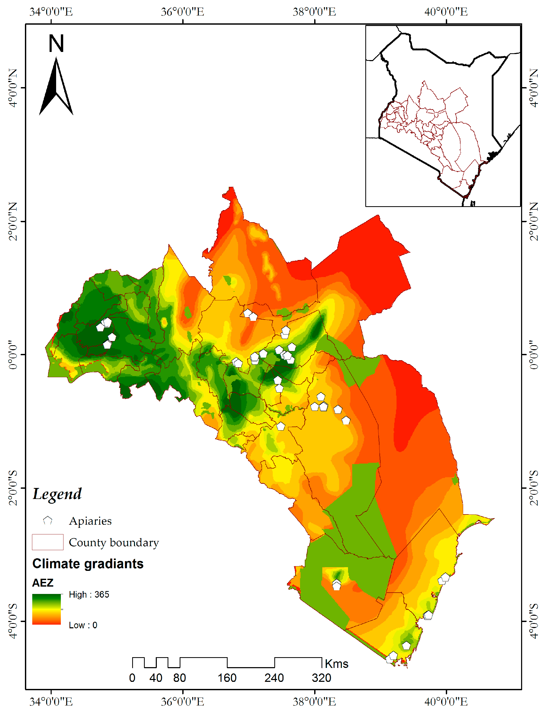
2.1. Study Sites
2.2. Occurrence Data
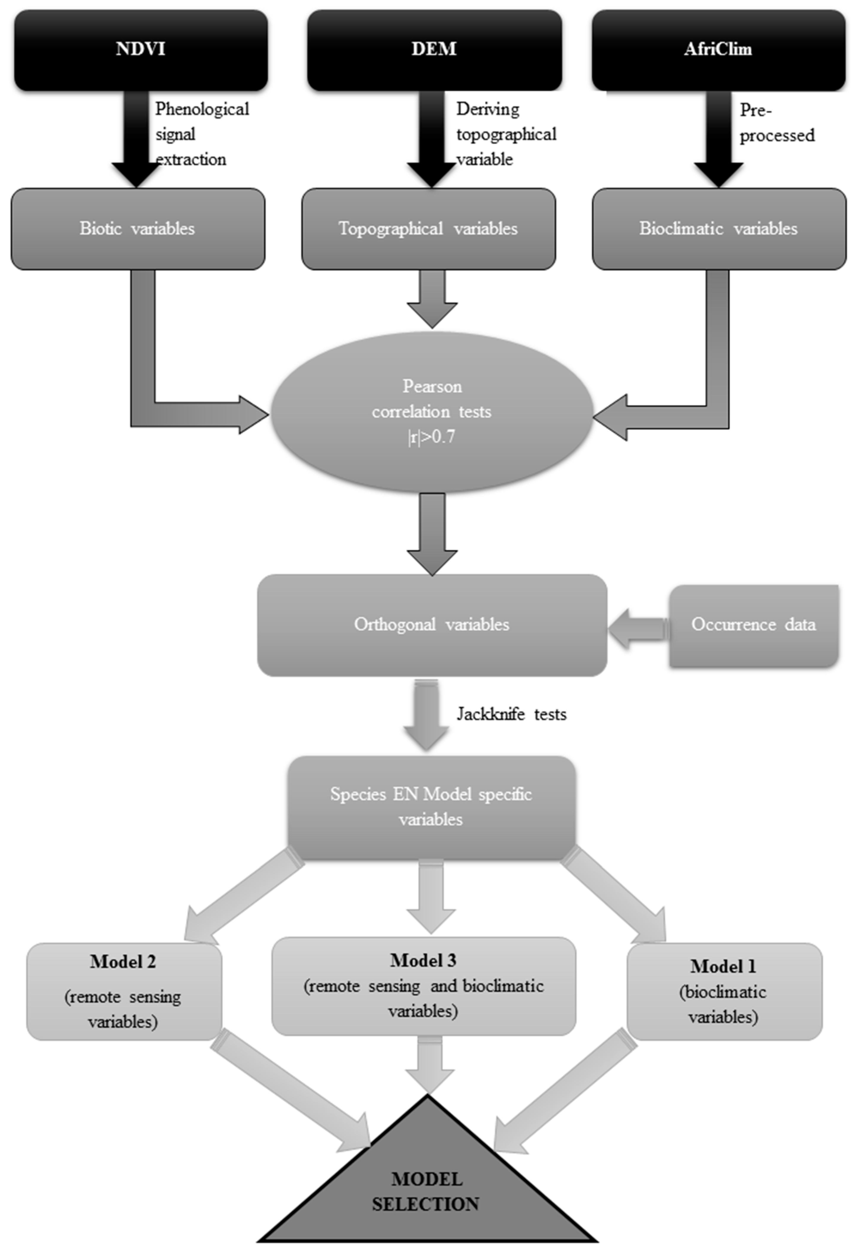
2.3. Preparation of Data for Analysis
2.4. Remotely Sensed Data Processing
2.4.1. Biotic Variables
2.4.2. Topographical Variables
2.5. Bioclimatic Data
2.6. Ecological Niche Modelling
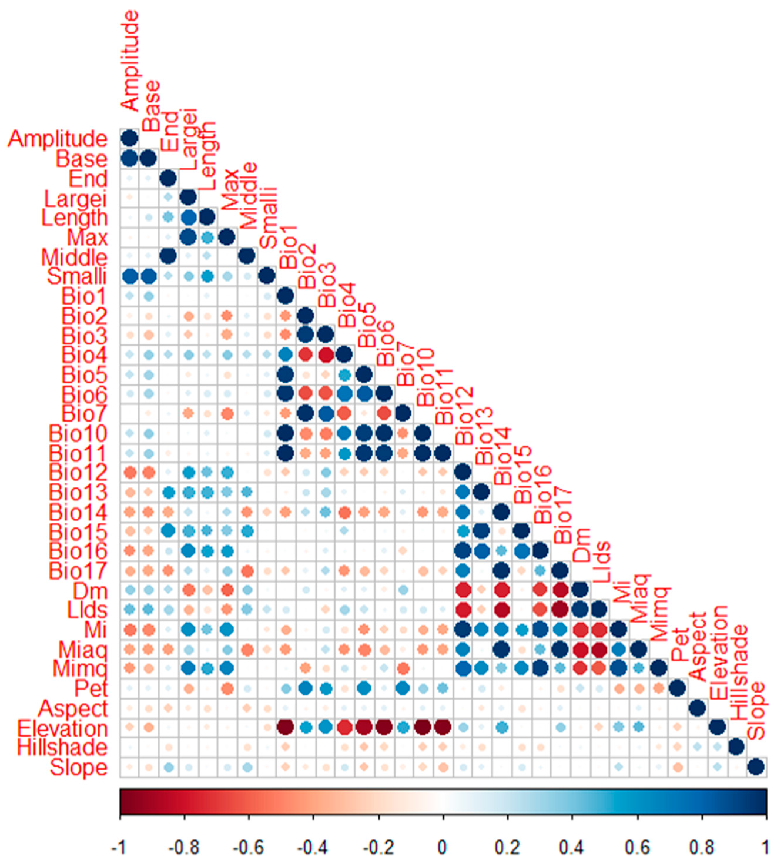
2.7. Variable Selection
2.8. Model Settings
2.9. Model Evaluation
3. Results
3.1. Honeybee Pest Abundance
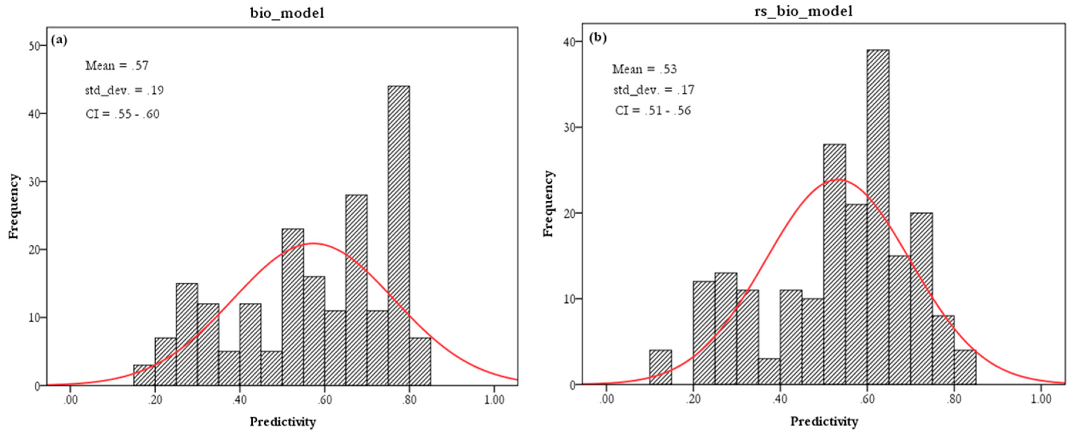
3.2. EN Models
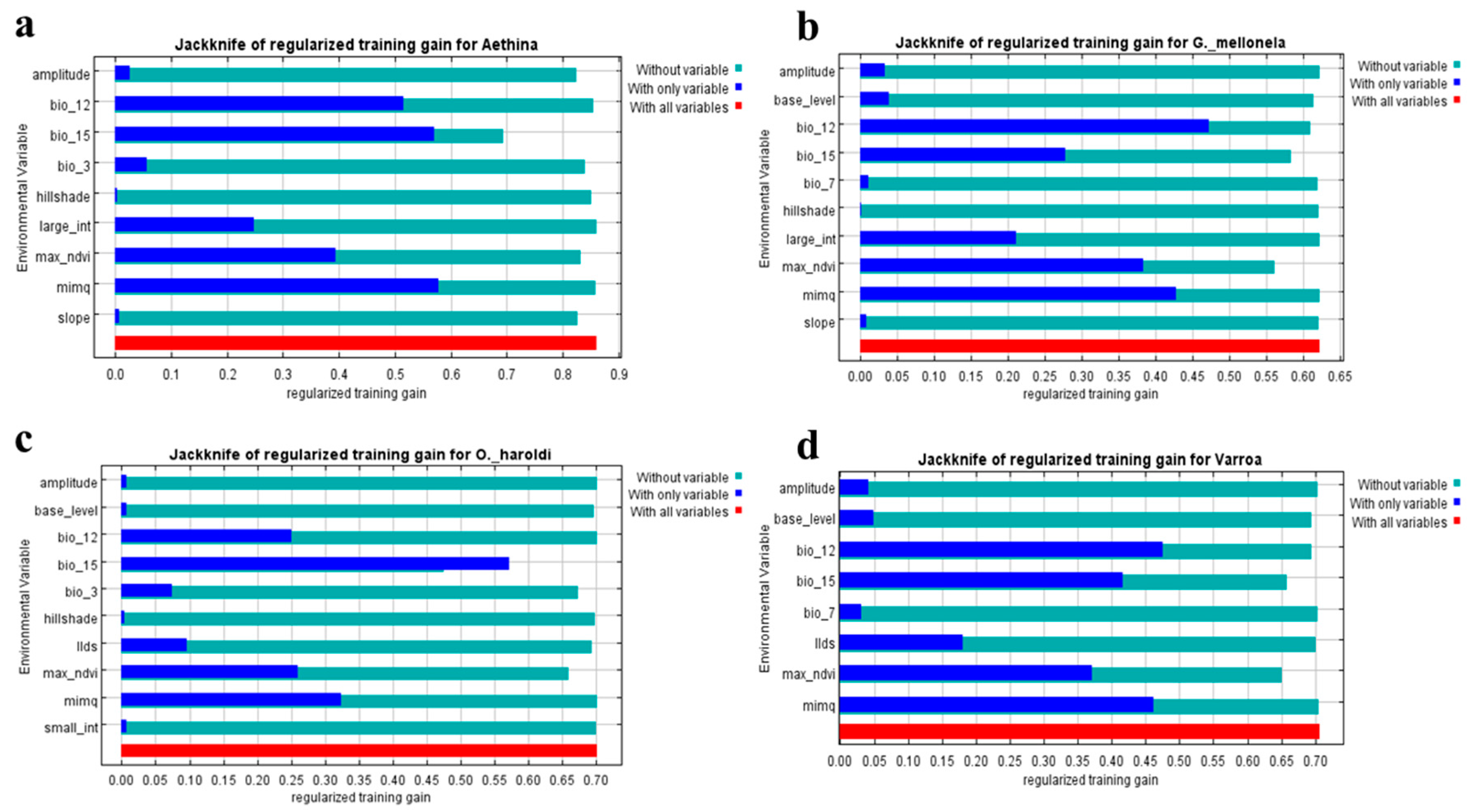
3.3. Predictor Variable Contribution
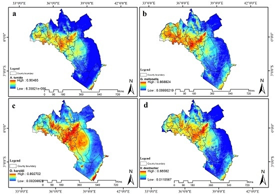
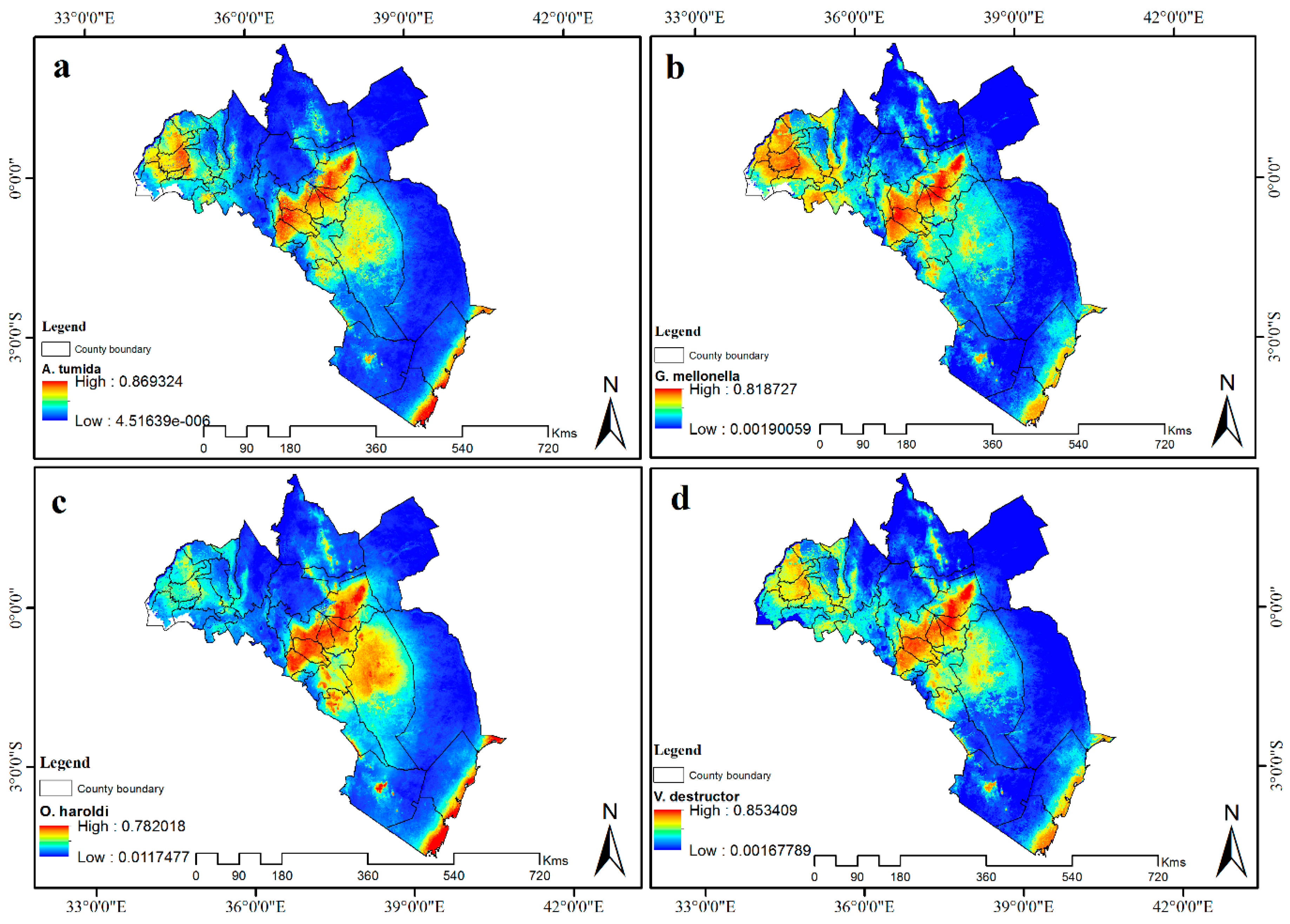
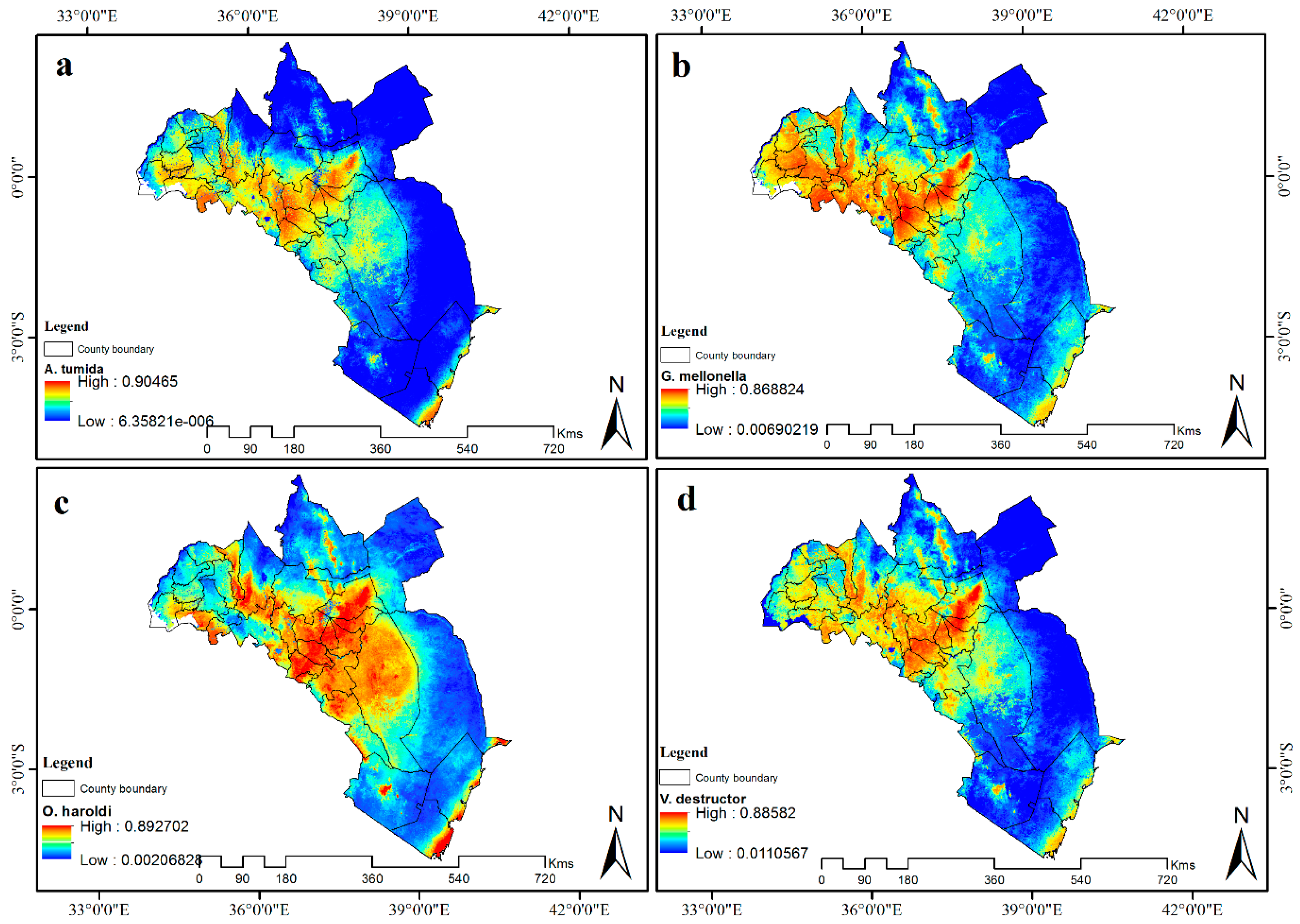
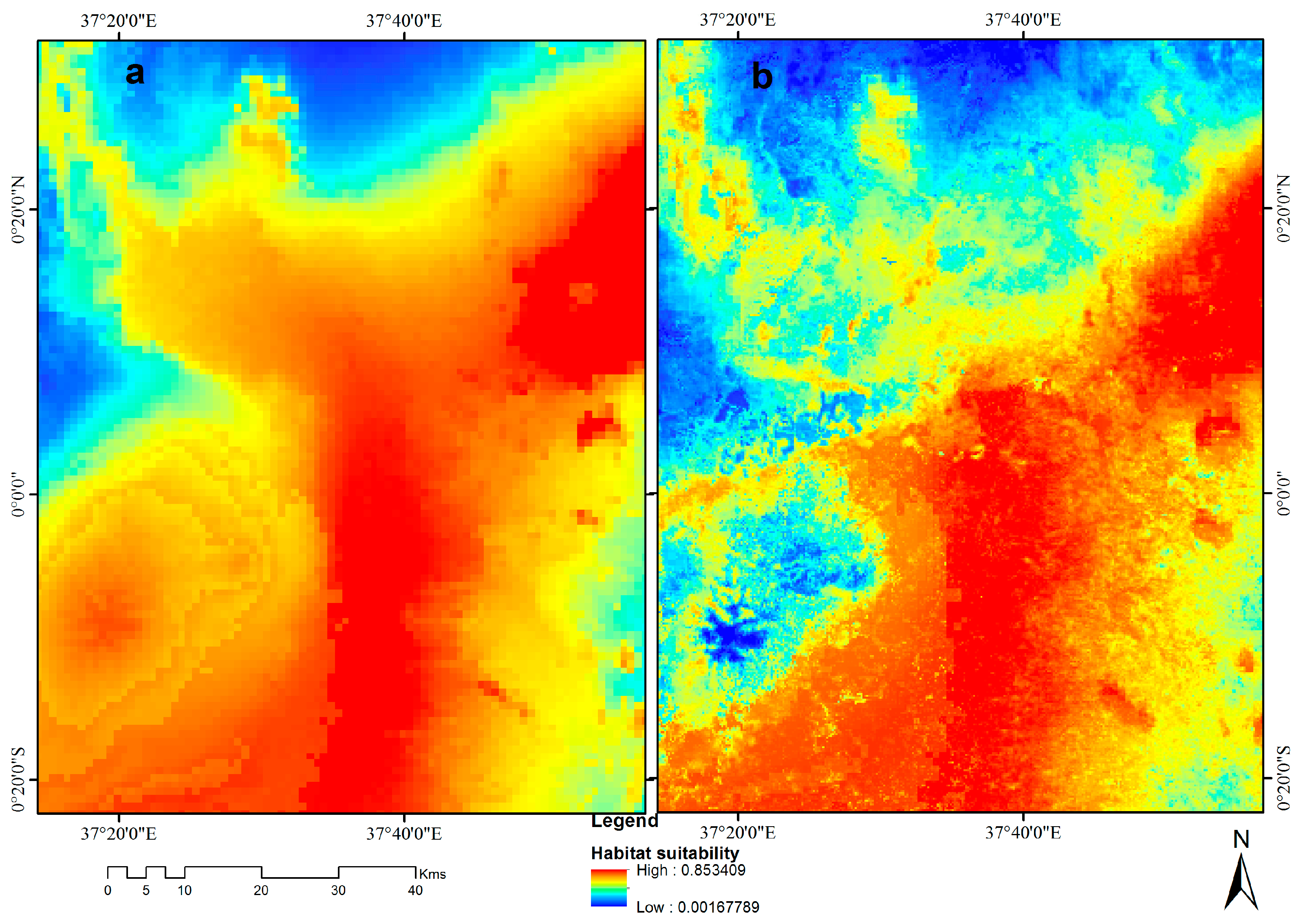
3.4. Visualization of Distribution
3.5. Contribution of Remotely Sensed Data
4. Discussion
4.1. Predictor Variable Contribution
4.2. Contribution of Remotely Sensed Data
4.3. Advantages of Using Integrative EN Models and Applicability
5. Conclusions
Acknowledgments
Author Contributions
Conflicts of Interest
References
- Kiatoko, N.; Raina, S.K.; Muli, E.; Mueke, J. Enhancement of fruit quality in Capsicum annum through pollination by Hypotrigona gribodoi in Kakamega, Western Kenya. Entomol. Sci. 2014, 17, 106–110. [Google Scholar] [CrossRef]
- Klein, A.-M.; Vaissière, B.E.; Cane, J.H.; Steffan-Dewenter, I.; Cunningham, S.A.; Kremen, C.; Tscharntke, T. Importance of pollinators in changing landscapes for world crops. Proc. R. Soc. London B: Biol. Sci. 2007, 274, 303–313. [Google Scholar] [CrossRef] [PubMed]
- Raina, S.K.; Kioko, E.; Zethner, O.; Wren, S. Forest habitat conservation in Africa using commercially important insects. Ann. Rev. Entomol. 2011, 56, 465–485. [Google Scholar] [CrossRef] [PubMed]
- Muli, E.; Patch, H.; Frazier, M.; Frazier, J.; Torto, B.; Baumgarten, T.; Kilonzo, J.; Kimani, J.N.; Mumoki, F.; Masiga, D. Evaluation of the distribution and impacts of parasites, pathogens, and pesticides on Honey Bee (Apis mellifera) Populations in East Africa. PLoS ONE 2014, 16, e94459. [Google Scholar] [CrossRef] [PubMed]
- Zayed, A. Bee genetics and conservation. Apidologie 2009, 40, 237–262. [Google Scholar] [CrossRef]
- Pirk, C.W.W.; Strauss, U.; Yusuf, A.A.; Démares, F.; Human, H. Honeybee health in Africa—A review. Apidologie 2015, 30, 1–25. [Google Scholar] [CrossRef]
- Fombong, A.T.; Mumoki, F.N.; Muli, E.; Masiga, D.K.; Arbogast, R.T.; Teal, P.E.; Torto, B. Occurrence, diversity and pattern of damage of Oplostomus species (Coleoptera: Scarabaeidae), honey bee pests in Kenya. Apidologie 2013, 44, 11–20. [Google Scholar] [CrossRef]
- Torto, B.; Fombong, A.T.; Mutyambai, D.M.; Muli, E.; Arbogast, R.T.; Teal, P.E.A. Aethina tumida (Coleoptera: Nitidulidae) and Oplostomus haroldi (Coleoptera: Scarabaeidae): Occurrence in Kenya, distribution within honey bee colonies, and responses to host odors. Ann. Entomol. Soc. Am. 2010, 103, 389–396. [Google Scholar] [CrossRef]
- Mumoki, F.N.; Fombong, A.; Muli, E.; Muigai, A.W.T.; Masiga, D. An inventory of documented diseases of African honeybees. Afr. Entomol. 2014, 22, 473–487. [Google Scholar] [CrossRef]
- Peterson, A.T.; Nakazawa, Y. Environmental data sets matter in ecological niche modelling: An example with Solenopsis invicta and Solenopsis richteri. Glob. Ecol. Biogeogr. 2008, 17, 135–144. [Google Scholar] [CrossRef]
- Neumann, P.; Ellis, J.D. The small hive beetle (Aethina tumida Murray, Coleoptera: Nitidulidae): distribution, biology and control of an invasive species. J. Apicult. Res. 2008, 47, 181–183. [Google Scholar] [CrossRef]
- Neumann, P.; Pirk, C.; Hepburn, H.; Solbrig, A.; Ratnieks, F.; Elzen, P.; Baxter, J. Social encapsulation of beetle parasites by Cape honeybee colonies (Apis mellifera capensis Esch). Naturwissenschaften 2001, 88, 214–216. [Google Scholar] [PubMed]
- Simone-Finstrom, M.D.; Spivak, M. Increased resin collection after parasite challenge: A case of Self-medication in honey bees? PLoS ONE 2012, 7, e34601. [Google Scholar] [CrossRef] [PubMed]
- Pau, S.; Gillespie, T.W.; Wolkovich, E.M. Dissecting NDVI–species richness relationships in Hawaiian dry forests. J. Biogeogr. 2012, 39, 1678–1686. [Google Scholar] [CrossRef]
- Fernández, M.; Hamilton, H. Ecological Niche Transferability Using Invasive Species as a Case Study. PLoS ONE 2015, 10, e0119891. [Google Scholar] [CrossRef] [PubMed]
- Kearney, M.; Porter, W. Mechanistic niche modelling: Combining physiological and spatial data to predict species’ ranges. Ecol. Lett. 2009, 12, 334–350. [Google Scholar] [CrossRef] [PubMed]
- Champetier, A.; Sumner, D.A.; Wilen, J.E. The bioeconomics of honey bees and pollination. Environ. Resour. Econ. 2014, 60, 143–164. [Google Scholar] [CrossRef]
- Peterson, A.T.; Ball, L.G.; Cohoon, K.P. Predicting distributions of Mexican birds using ecological niche modelling methods. Int. J. Avian Sci. 2002, 144, E27–E32. [Google Scholar] [CrossRef]
- Phillips, S.J.; Dudík, M. Modeling of species distributions with Maxent: New extensions and a comprehensive evaluation. Ecography 2008, 31, 161–175. [Google Scholar] [CrossRef]
- Cord, A.F.; Klein, D.; Gernandt, D.S.; de la Rosa, J.A.P.; Dech, S. Remote sensing data can improve predictions of species richness by stacked species distribution models: A case study for Mexican pines. J. Biogeogr. 2014, 41, 736–748. [Google Scholar] [CrossRef]
- Neumann, P.; Pettis, J.S.; Schäfer, M.O. Quo vadis Aethina tumida? Biology and control of small hive beetles. Apidologie 2016, 47, 427–466. [Google Scholar] [CrossRef] [Green Version]
- Speranza, C.I.; Kiteme, B.; Ambenje, P.; Wiesmann, U.; Makali, S. Indigenous knowledge related to climate variability and change: Insights from droughts in semi-arid areas of former Makueni District, Kenya. Climate Chang. 2009, 100, 295–315. [Google Scholar] [CrossRef]
- Githui, F.; Gitau, W.; Mutua, F.; Bauwens, W. Climate change impact on SWAT simulated streamflow in western Kenya. Int. J. Climatol. 2009, 29, 1823–1834. [Google Scholar] [CrossRef]
- Dietemann, V.; Nazzi, F.; Martin, S.J.; Anderson, D.L.; Locke, B.; Delaplane, K.S. Standard methods for varroa research. J. Apic. Res. 2013, 52, 1–54. [Google Scholar] [CrossRef]
- Haredasht, A.S.; Barrios, M.; Farifteh, J.; Maes, P.; Clement, J.; Verstraeten, W.W.; Tersago, K.; Van Ranst, M.; Coppin, P.; Berckmans, D. Ecological niche modelling of Bank Voles in Western Europe. Int. J. Environ. Res. Public Health 2013, 10, 499–514. [Google Scholar] [CrossRef] [PubMed]
- Merow, C.; Smith, M.J.; Silander, J.A. A practical guide to MaxEnt for modeling species’ distributions: What it does, and why inputs and settings matter. Ecography 2013, 36, 1058–1069. [Google Scholar] [CrossRef]
- Eklundha, L.; Jönsson, P. TIMESAT 3.1 Software Manual; Lund University: Lund, Sweden, 2012. [Google Scholar]
- Jönsson, P.; Eklundh, L. TIMESAT—A program for analyzing time-series of satellite sensor data. Comput. Geosci. 2004, 30, 833–845. [Google Scholar] [CrossRef]
- Clark, M.L.; Aide, T.M.; Grau, H.R.; Riner, G. A scalable approach to mapping annual land cover at 250 m using MODIS time series data: A case study in the Dry Chaco ecoregion of South America. Remote Sens. Environ. 2010, 114, 2816–2832. [Google Scholar] [CrossRef]
- Jamali, S.; Jönsson, P.; Eklundh, L.; Ardö, J.; Seaquist, J. Detecting changes in vegetation trends using time series segmentation. Remote Sens. Environ. 2015, 156, 182–195. [Google Scholar] [CrossRef]
- Foi, A.; Trimeche, M.; Katkovnik, V.; Egiazarian, K. Practical Poissonian-Gaussian noise modeling and fitting for single-image raw-data. IEEE Trans. Image Process. 2008, 17, 1737–1754. [Google Scholar] [CrossRef] [PubMed]
- Shen, Y.; Wu, L.; Di, L.; Yu, G.; Tang, H.; Yu, G.; Shao, Y. Hidden Markov models for real-time estimation of corn progress stages using MODIS and meteorological data. Remote Sens. 2013, 5, 1734–1753. [Google Scholar] [CrossRef]
- Fu, X.; Wang, L. Data dimensionality reduction with application to simplifying RBF network structure and improving classification performance. IEEE Trans. Syst. Man. Cybern. Part B: Cybern. 2003, 33, 399–409. [Google Scholar]
- Hinton, G.E.; Salakhutdinov, R.R. Reducing the dimensionality of data with neural networks. Science 2006, 313, 504–507. [Google Scholar] [CrossRef] [PubMed]
- Jarvis, A.; Reuter, H.I.; Nelson, A.; Guevara, E. Hole-filled SRTM for the globe Version 4. The CGIAR-CSI SRTM 90 m Database. 2008. Available online: http://srtm.csi.cgiar.org/ (accessed on 2 March 2015).
- Platts, P.J.; Omeny, P.A.; Marchant, R. AFRICLIM: High-resolution climate projections for ecological applications in Africa. Afr. J. Ecol. 2015, 53, 103–108. [Google Scholar] [CrossRef]
- Lovett, J.C. Modelling the effects of climate change in Africa. Afr. J. Ecol. 2015, 53, 1–2. [Google Scholar] [CrossRef]
- Mwalusepo, S.; Tonnang, H.E.Z.; Massawe, E.S.; Okuku, G.O.; Khadioli, N.; Johansson, T.; Calatayud, P.-A.; Ru, B.P.L. Predicting the impact of temperature change on the future distribution of Maize Stem Borers and their natural enemies along East African Mountain gradients using phenology models. PLoS ONE 2015, 10, e0130427. [Google Scholar] [CrossRef] [PubMed]
- IPCC. Climate Change 2013—The physical science basis: Working group I contribution to the fifth assessment report of the intergovernmental panel on climate change. In Intergovernmental Panel on Climate Change; Cambridge University Press: Cambridge, UK, 2013; Available online: http://ebooks.cambridge.org/ref/id/CBO9781107415324 (accessed on 3 October 2015).
- Phillips, S.J.; Anderson, R.P.; Schapire, R.E. Maximum entropy modeling of species geographic distributions. Ecol. Model. 2006, 190, 231–259. [Google Scholar] [CrossRef]
- Rodríguez-Castañeda, G.; Hof, A.R.; Jansson, R.; Harding, L.E. Predicting the fate of biodiversity using species’ distribution models: Enhancing model comparability and repeatability. PLoS ONE 2012, 7, e44402. [Google Scholar] [CrossRef] [PubMed]
- Peterson, A.T.; Papeş, M.; Eaton, M. Transferability and model evaluation in ecological niche modeling: A comparison of GARP and Maxent. Ecography 2007, 30, 550–560. [Google Scholar] [CrossRef]
- Ward, G.; Hastie, T.; Barry, S.; Elith, J.; Leathwick, J.R. Presence-only data and the EM algorithm. Biometrics 2009, 65, 554–563. [Google Scholar] [CrossRef] [PubMed]
- Dormann, C.F.; Elith, J.; Bacher, S.; Buchmann, C.; Carl, G.; Carré, G.; García Marquéz, J.R.; Gruber, B.; Lafourcade, B.; Leitão, P.J.; et al. Collinearity: A review of methods to deal with it and a simulation study evaluating their performance. Ecography 2013, 36, 27–46. [Google Scholar] [CrossRef]
- Peterson, A.T.; Cohoon, K.P. Sensitivity of distributional prediction algorithms to geographic data completeness. Ecol. Model. 1999, 117, 159–164. [Google Scholar] [CrossRef]
- Yackulic, C.B.; Chandler, R.; Zipkin, E.F.; Royle, J.A.; Nichols, J.D.; Campbell Grant, E.H.; Veran, S. Presence-only modelling using MAXENT: When can we trust the inferences? Methods Ecol. Evol. 2013, 4, 236–243. [Google Scholar] [CrossRef]
- Du, Z.; Wang, Z.; Liu, Y.; Wang, H.; Xue, F.; Liu, Y. Ecological niche modeling for predicting the potential risk areas of severe fever with thrombocytopenia syndrome. Int. J. Infect. Dis. 2014, 26, 1–8. [Google Scholar] [CrossRef] [PubMed]
- Swets, J.A. Measuring the accuracy of diagnostic systems. Science 1988, 240, 1285–1293. [Google Scholar] [CrossRef] [PubMed]
- Raes, N.; ter Steege, H. A null-model for significance testing of presence-only species distribution models. Ecography 2007, 30, 727–736. [Google Scholar] [CrossRef]
- Hernandez, P.A.; Graham, C.H.; Master, L.L.; Albert, D.L. The effect of sample size and species characteristics on performance of different species distribution modeling methods. Ecography 2006, 29, 773–785. [Google Scholar] [CrossRef]
- Martin, S.J.; Highfield, A.C.; Brettell, L.; Villalobos, E.M.; Budge, G.E.; Powell, M.; Schroeder, D.C. Global honey bee viral landscape altered by a parasitic mite. Science 2012, 336, 1304–1306. [Google Scholar] [CrossRef] [PubMed]
- Strauss, U.; Human, H.; Gauthier, L.; Crewe, R.M.; Dietemann, V.; Pirk, C.W. Seasonal prevalence of pathogens and parasites in the savannah honeybee (Apis mellifera scutellata). J. Invertebr. Pathol. 2013, 114, 45–52. [Google Scholar] [CrossRef] [PubMed]
- Raina, S.K.; Kimbu, D.M. Variations in races of the honeybee Apis mellifera (Hymenoptera: Apidae) in Kenya. Int. J. Trop. Insect Sci. 2005, 25, 281–291. [Google Scholar] [CrossRef]
- Wiley, E.O.; McNyset, K.M.; Peterson, A.T.; Robins, C.R.; Stewart, A.M. Niche modeling perspective on geographic range predictions in the marine environment using a machine-learning algorithm. Oceanography 2003, 16, 120–127. [Google Scholar] [CrossRef]
- Mani, M.S. Ecology and Biogeography of High Altitude Insects; Springer Science & Business Media: Berlin, Germany, 2013; p. 539. [Google Scholar]
- Aranda, S.C.; Lobo, J.M. How well does presence-only-based species distribution modelling predict assemblage diversity? A case study of the Tenerife flora. Ecography 2011, 34, 31–38. [Google Scholar] [CrossRef]
- Saatchi, S.; Buermann, W.; Ter Steege, H.; Mori, S.; Smith, T.B. Modeling distribution of Amazonian tree species and diversity using remote sensing measurements. Remote Sens. Environ. 2008, 112, 2000–2017. [Google Scholar] [CrossRef]
- Attorre, F.; Alfo, M.; De Sanctis, M.; Francesconi, F.; Bruno, F. Comparison of interpolation methods for mapping climatic and bioclimatic variables at regional scale. Int. J. Climatol. 2007, 27, 1825–1843. [Google Scholar] [CrossRef]
- Hijmans, R.J.; Cameron, S.E.; Parra, J.L.; Jones, P.G.; Jarvis, A. Very high resolution interpolated climate surfaces for global land areas. Int. J. Climatol. 2005, 25, 1965–1978. [Google Scholar] [CrossRef]
- Engler, R.; Guisan, A.; Rechsteiner, L. An improved approach for predicting the distribution of rare and endangered species from L occurrence and pseudo-absence data. J. Appl. Ecol. 2004, 41, 263–274. [Google Scholar] [CrossRef]
- Bradley, B.A.; Olsson, A.D.; Wang, O.; Dickson, B.G.; Pelech, L.; Sesnie, S.E.; Zachmann, L.J. Species detection vs. habitat suitability: Are we biasing habitat suitability models with remotely sensed data? Ecol. Model. 2012, 244, 57–64. [Google Scholar] [CrossRef]
- Clifford, G.D.; Tarassenko, L. Quantifying errors in spectral estimates of HRV due to beat replacement and resampling. IEEE Trans. Biomed. Eng. 2005, 52, 630–638. [Google Scholar] [CrossRef] [PubMed]
- Dikshit, O.; Roy, D.P. An empirical investigation of image resampling effects upon the spectral and textural supervised classification of a high spatial resolution multispectral image. Photogramm. Eng. Remote Sens. 1996, 62, 1085–1092. [Google Scholar]
- Fielding, A.H.; Bell, J.F. A review of methods for the assessment of prediction errors in conservation presence/absence models. Environ. Conserv. 1997, 24, 38–49. [Google Scholar] [CrossRef]
- Abdel-Rahman, E.M.; Makori, D.M.; Landmann, T.; Piiroinen, R.; Gasim, S.; Pellikka, P.; Raina, S.K. The utility of AISA eagle hyperspectral data and random forest classifier for flower mapping. Remote Sens. 2015, 7, 13298–13318. [Google Scholar] [CrossRef]
- Landmann, T.; Piiroinen, R.; Makori, D.M.; Abdel-Rahman, E.M.; Makau, S.; Pellikka, P.; Raina, S.K. Application of hyperspectral remote sensing for flower mapping in African savannas. Remote Sens. Environ. 2015, 166, 50–60. [Google Scholar] [CrossRef]


| Variable | Description | Units | Year | |
|---|---|---|---|---|
| Name | Abbreviation | |||
| A) Remotely sensed variables | ||||
| 1. Biotic Variables | ||||
| Start of the season | seas_start | Time for the start of the season | decades | 2001–2014 |
| End of the season | seas_end | Time for the end of the season | decades | 2001–2014 |
| Length of the season | seas_length | Length of the season from start to end | decades | 2001–2014 |
| Mid of the season | seas_mid | Mid of the season | decades | 2001–2014 |
| Base level | base_level | Average minimum NDVI value | n/a | 2001–2014 |
| Maximum NDVI | max_ndvi | Largest NDVI value in the season | n/a | 2001–2014 |
| Amplitude | amplitude | Difference between maximum and base level | n/a | 2001–2014 |
| Left derivative | left_der | Rate of increase at the beginning of season | % | 2001–2014 |
| Right derivative | right_der | Rate of decrease at the end of season | % | 2001–2014 |
| Large integral | large_int | Large season integral | n/a | 2001–2014 |
| Small integral | small_int | Small season integral | n/a | 2001–2014 |
| Number of seasons | num_seas | Number of seasons within the year | number | 2001–2014 |
| 2. Topographical variables | ||||
| Slope | slope | Steepness of the ground | % rise | |
| Aspect | aspect | Slope direction | degrees | |
| Hillshade | hillshade | Shading effect | n/a | |
| Elevation | elevation | Ground height | m | |
| B) Bioclimatic data | ||||
| 1. Temperature variables | ||||
| Bio 1 | bio1 | Mean annual temperature | °C | 1961–1990 |
| Bio 2 | bio2 | Mean diurnal range in temperature | °C | 1961–1990 |
| Bio 3 | bio3 | Isothermality | °C | 1961–1990 |
| Bio 4 | bio4 | Temperature seasonality | °C | 1961–1990 |
| Bio 5 | bio5 | Max temp warmest month | °C | 1961–1990 |
| Bio 6 | bio6 | Min temp coolest month | °C | 1961–1990 |
| Bio 7 | bio7 | Annual temp range | °C | 1961–1990 |
| Bio 10 | bio10 | Mean temp warmest quarter | °C | 1961–1990 |
| Bio 11 | bio11 | Mean temp coolest quarter | °C | 1961–1990 |
| Potential evapotranspiration | pet | Potential evapotranspiration | mm | 1961–1990 |
| 2. Precipitation variables | ||||
| Bio 12 | bio12 | Mean annual rainfall | mm | 1961–1990 |
| Bio 13 | bio13 | Rainfall wettest month | mm | 1961–1990 |
| Bio 14 | bio14 | Rainfall driest month | mm | 1961–1990 |
| Bio 15 | bio15 | Rainfall seasonality | mm | 1961–1990 |
| Bio 16 | bio16 | Rainfall wettest quarter | mm | 1961–1990 |
| Bio 17 | bio17 | Rainfall driest quarter | mm | 1961–1990 |
| Moisture index | mi | Annual moisture index | n/a | 1961–1990 |
| Moisture index moist quarter | mimq | Moisture index moist quarter | n/a | 1961–1990 |
| Moisture index arid quarter | miaq | Moisture index arid quarter | n/a | 1961–1990 |
| Dry months | dm | Number of dry months | month | 1961–1990 |
| Length of longest dry season | llds | Length of longest dry season | month | 1961–1990 |
| A. tumida | G. mellonella | O. haroldi | V. destructor | |
|---|---|---|---|---|
| Wet season | 272a | 20a | 31a | 476a |
| Dry season | 58b | 21a | 15b | 75b |
| Model 1 | Model 2 | Model 3 | ||||
|---|---|---|---|---|---|---|
| AUC | SD | AUC | SD | AUC | SD | |
| A. tumida | 0.85 | ±0.08 | 0.80 | ±0.07 | 0.87 | ±0.07 |
| G. mellonella | 0.80 | ±0.11 | 0.75 | ±0.09 | 0.80 | ±0.08 |
| O. haroldi | 0.85 | ±0.10 | 0.76 | ±0.16 | 0.87 | ±0.09 |
| V. destructor | 0.83 | ±0.08 | 0.76 | ±0.09 | 0.88 | ±0.07 |
| A. tumida | G. mellonella | O. haroldi | V. destructor | |
|---|---|---|---|---|
| Remotely sensed variables (biotic variables) | ||||
| amplitude | 4.3 | 2.0 | 0.7 | 6.3 |
| base_level | - | 8.9 | 1.5 | 6.1 |
| large_int | 0.8 | 0.5 | - | - |
| max_ndvi | 7.7 | 29.4 | 8.3 | 19.3 |
| small_int | - | - | 0.9 | - |
| RS (biotic) total | 12.8 | 40.8 | 11.4 | 31.7 |
| Remotely sensed variables (topographical variables) | ||||
| hillshade | 1.2 | 0.2 | 0.5 | - |
| slope | 3.0 | 0.3 | - | - |
| Topographical total | 4.2 | 0.5 | 0.5 | - |
| Bioclimatic variables (precipitation and temperature variables) | ||||
| bio3 | 2.0 | - | 7.3 | - |
| bio7 | - | 0.7 | - | 20.5 |
| bio12 | 1.7 | 13.7 | - | 20.5 |
| bio15 | 43.9 | 11.9 | 79.7 | 28.2 |
| llds | - | - | 1.1 | 0.5 |
| mimq | 35.4 | 32.4 | - | 18.7 |
| Bioclimatic total | 83.0 | 58.7 | 88.1 | 68.3 |
| Grand total | 100 | 100 | 100 | 100 |
© 2017 by the authors. Licensee MDPI, Basel, Switzerland. This article is an open access article distributed under the terms and conditions of the Creative Commons Attribution (CC BY) license ( http://creativecommons.org/licenses/by/4.0/).
Share and Cite
Makori, D.M.; Fombong, A.T.; Abdel-Rahman, E.M.; Nkoba, K.; Ongus, J.; Irungu, J.; Mosomtai, G.; Makau, S.; Mutanga, O.; Odindi, J.; et al. Predicting Spatial Distribution of Key Honeybee Pests in Kenya Using Remotely Sensed and Bioclimatic Variables: Key Honeybee Pests Distribution Models. ISPRS Int. J. Geo-Inf. 2017, 6, 66. https://doi.org/10.3390/ijgi6030066
Makori DM, Fombong AT, Abdel-Rahman EM, Nkoba K, Ongus J, Irungu J, Mosomtai G, Makau S, Mutanga O, Odindi J, et al. Predicting Spatial Distribution of Key Honeybee Pests in Kenya Using Remotely Sensed and Bioclimatic Variables: Key Honeybee Pests Distribution Models. ISPRS International Journal of Geo-Information. 2017; 6(3):66. https://doi.org/10.3390/ijgi6030066
Chicago/Turabian StyleMakori, David M., Ayuka T. Fombong, Elfatih M. Abdel-Rahman, Kiatoko Nkoba, Juliette Ongus, Janet Irungu, Gladys Mosomtai, Sospeter Makau, Onisimo Mutanga, John Odindi, and et al. 2017. "Predicting Spatial Distribution of Key Honeybee Pests in Kenya Using Remotely Sensed and Bioclimatic Variables: Key Honeybee Pests Distribution Models" ISPRS International Journal of Geo-Information 6, no. 3: 66. https://doi.org/10.3390/ijgi6030066